Two States for Optimal Position and Capacity of Distributed Generators Considering Network Reconfiguration for Power Loss Minimization Based on Runner Root Algorithm

Abstract

Although the distributed generator (DG) placement and distribution network (DN) reconfiguration techniques contribute to reduce power loss, obviously the former is a design problem which is used for a long-term purpose while the latter is an operational problem which is used for a short-term purpose. In this situation, the optimal value of the position and capacity of DGs is a value which must be not affected by changing the operational configuration due to easy changes in the status of switches compared with changes in the installed location of DG. This paper demonstrates a methodology for choosing the position and size of DGs on the DN that takes into account re-switching the status of switches on distribution of the DN to reduce power losses. The proposed method is based on the runner root algorithm (RRA) which separates the problem into two states. In State-I, RRA is used to optimize the position and size of DGs on closed-loop distribution networks which is a mesh shape topology and power is delivered through more than one line. In State-II, RRA is used to reconfigure the DN after placing the DGs to find the open-loop distribution network which is a tree shape topology and power is only delivered through one line. The calculation results in DN systems with 33 nodes and 69 nodes, showing that the proposed method is capable of solving the problem of the optimal position and size of DGs considering distribution network reconfiguration.

1. Introduction

The distribution system has a radial or mesh configuration but operates in radial state. The power flow in this case flows from the system through the distribution network to the load. Therefore, the transmission of power from the power plant to the consumer will generate losses on the transmission and distribution network. With the new distribution grid structure, due to the involvement of DGs, power flow is not only flowing from the transmission system but also circulating between parts of the distribution network back to the transmission grid. With the involvement of DGs, the distribution network performs better in the task of providing electricity to the consumer, assuring the quality of power, the reliability of the power supply as well as reduced load on the network, improved voltage, reduced power losses, reduced power losses and support grid.

DGs are linked to the electric distributed system. Because of their huge economical benefit and energy security, the appearance of DGs on distribution systems has been rising quickly [1,2]. In addition, for large-capacity DGs using renewable energy sources such as wind and solar cells are often connected to the transmission network. As unfavorable environmental conditions such as a lack of wind or sun can lead to power shortages on the transmission network for supplying to th distribution network, finding solutions to compensate for this shortfall of power are very importance for DG suppliers, especially in the competitive electricity market. One of the most effective solutions to this problem is the installation of small-capacity DGs based on diesel fuel, heavy oil, fuel cell, natural gas, etc. in the DN to compensate for the shortfall of power. Therefore, selection of the optimal installation position for these types of DG to reduce power losses and improve the efficiency of the DN is important. There are several studies which have been proposed for the problem of positioning and size with the goal of reducing losses on the network. The main method based on analytical approaches such as the improved analytical method [3,4,5] or meta-heuristic algorithms like genetic algorithm (GA) [6,7], particle swarm optimization algorithm (PSO) [8,9] the hybrid big bang-big crunch algorithm (HBB-BC) [10], hybrid teaching–learning-based optimization (HTLBO) [11], invasive weed optimization (IWO) [12], cuckoo search algorithm (CSA) [13], fireworks algorithm (FWA) [14], harmony search algorithm (HSA) [15], and adaptive weighted improved discrete particle swarm optimization (AWIDPSO) [16]. In [3,4,5,6,7,8,9,10,11,12], the authors only focused on optimizing the position and capacity of DGs on the DN without considering configuration of the DN which is also an effective technique for reduction power loss in the DN system. This technique called distribution network reconfiguration (DNR) is performed by changing the closed/open status of sectionalizing and tie switches while respecting system constraints [17]. Merlin and Back [18] were the first authors proposed the DNR problem and solved it by the discrete branch-and-bound type heuristic technique. The switch exchange method for loss reduction was proposed by Civanlar et al. [19]. Due to the based on heuristics methods, it is difficult to reach an optimal solution. In recent, new methods based on meta-heuristic have been proposed for finding an optimal network configuration. In [20], the DNR problem for minimizing power loss and enhancing system reliability is solved by an enhanced genetic algorithm. In the study, the crossover and mutation operations have been improved to determine the opened switches. In [21], a binary gravitational search algorithm was proposed for the multi-objective DNR problem. In [22], a binary group search optimization was applied to solve the DNR problem for power loss reduction. In [23], a fireworks algorithm has been performed to reduce power loss and enhance voltage of nodes. In [24], a shuffled frog leaping algorithm was used for minimizing the cost of power loss and power of distributed generators. In [8], a discrete artificial bee colony has presented for the DNR problem. In [25], a particle swarm optimization was presented to handle the DNR problem with multi-objective functions. In [26], a reconfiguration method based on adapted ant colony optimization was proposed for minimization of power loss.

On the DN system-integrated DGs, the operating configuration of the DN system will be changed by using the DNR technique. As the network configuration changes, the location of the DGs which is defined before that can be unsuitable to reduce losses and promote voltage stability or the unsuitable capacity of the DGs will cause large losses on the DN. Therefore, in recent years, some studies have combined both the DG placement problems and distribution network reconfiguration to enhance the effectiveness of the electric distribution system [13,14,15,16]. Although both techniques contribute to reduce power loss, obviously the DG placement problem is a design problem of the distribution network which is used for a long-term purpose while the distribution network reconfiguration problem is an operational problem of the distribution network which is used for a short-term purpose. In this situation, the optimal value of position and capacity of DGs is a value which must be not affected by the changing of operational configuration because changing the status of switches is easier than changing the location of DG as they are installed. This requirement is unnecessary by solving simultaneously both problems because the optimal position and size of DG will be change when the location of open switches on the DN change. In addition, by solving combined problems, the parameters of the optimization algorithm will be become more complex than those of solving individual problems. An illustration for this point can be seen in that the control variables will be lengthier and it will take more time and more iterations for finding optimal solution.

Therefore, in this article we propose the method of determining the position and size of the DGs on the DN, considering the problem of distribution network reconfiguration with the goal of reducing power losses. The proposed method of determining the optimal location and size of DGs and operational configurations are implemented in two states based on the runner-root algorithm (RRA). In State-I, RRA is used to identify the optimal position and capacity of the DGs on the closed-loop distribution network. In State-II, the RRA is used to find the optimal operating configuration of the system. By using the proposed method for the combined problem of placement of the DG and re-switching, in the obtained results, the position and size of the DG is not affected by the location of open switches. It means that the design problem which is the placement DG problem is not be depended by the operational problem which is the re-switching problem. In addition, by solving individual problems, it also helps the optimization algorithms be more effective at finding the optimal solution in two states. The comparison results on 33 and 69 nodes systems with the method of solving simultaneously the combined problem and other studied methods have shown that the proposed method is capable of solving the problem of the optimal position and size of DGs considering distribution network reconfiguration. In the following section, the proposed distribution network reconfiguration method for the optimal location and size of the DG considering network reconfiguration for power loss is presented. The overview of RRA for the problem is demonstrated in Section 3. Section 4 presents the calculated results of the suggested algorithm and the conclusion are presented in Section 5.

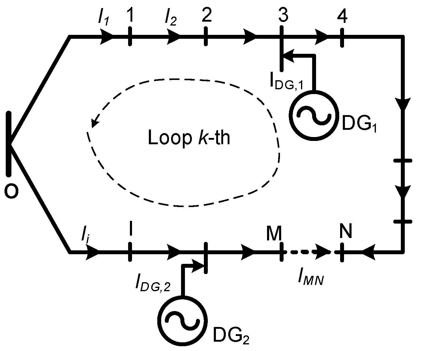
2. Problem Formulation

The distribution networks are usually designed in a mesh structure but they are operated in open status. The change of power loss when they are transferred from the mesh status to the radial status is described as follows:

The distribution network reconfiguration problem will be demonstrated by the simple network shown in Figure 1. If the switch MN is closed, the system is operating in the mesh network configuration. Calling the current on the branch ith is I_i (i = 1, …, nbr). When the switch MN is opened, assuming that the current on the branches of the OM decreases by I_MN, the current on the branches of ON will increase by I_MN. Then, power loss of the mesh network (ΔP^mesh) and power loss of the radial network (ΔP^radial) are expressed by Equations (1) and (2) respectively.

$$\Delta P^{mesh}={\displaystyle \sum }_{i\in OM}^{nbr}{R}_i{I}_i^2+R_{MN}{I}_{MN}^2+{\displaystyle \sum }_{i\in ON}^{nbr}{\left(-I_i\right)}^2{R}_i$$

(1)

$$\Delta P^{radial}={\displaystyle \sum }_{i\in OM}^{nbr}{R}_i{\left(I_i-I_{MN}\right)}^2+{\displaystyle \sum }_{i\in ON}^{nbr}{R}_i{\left(I_i+I_{MN}\right)}^2$$

(2)

The effect of the reconfiguration (change in power losses in the loop) can be obtained by using (3):

$$\begin{array}{l}\Delta P^{radial}-\Delta P^{mesh}\\ ={\displaystyle {\displaystyle \sum }_{i\in OM}^{nbr}}{R}_i\left(I_i^2-2I_{MN}{I}_i+I_{MN}^2\right)+{\displaystyle {\displaystyle \sum }_{i\in ON}^{nbr}}{R}_i\left(I_i^2+2I_{MN}{I}_i+I_{MN}^2\right)\\ -{\displaystyle {\displaystyle \sum }_{i\in OM}^{nbr}}{R}_i{I}_i^2-R_{MN}{I}_{MN}^2-{\displaystyle {\displaystyle \sum }_{i\in ON}^{nbr}}{\left(I_i\right)}^2{R}_i\end{array}$$

(3)

$$\begin{array}{l}\Delta P^{radial}-\Delta P^{mesh}\\ ={\displaystyle {\displaystyle \sum }_{i\in OM}^{nbr}}{R}_i\left(-2I_{MN}{I}_i+I_{MN}^2\right)+{\displaystyle {\displaystyle \sum }_{i\in ON}^{nbr}}{R}_i\left(2I_{MN}{I}_i+I_{MN}^2\right)-R_{MN}{I}_{MN}^2+R_{MN}{I}_{MN}^2\\ -R_{MN}{I}_{MN}^2\end{array}$$

(4)

Short (4), resulting in (5):

$$\begin{array}{l}\Delta P^{radial}-\Delta P^{mesh}\\ =I_{MN}^2\left({\displaystyle {\displaystyle \sum }_{i\in OM}^{nbr}}{R}_i+R_{MN}+{\displaystyle {\displaystyle \sum }_{i\in ON}^{nbr}}{R}_i\right)\\ -2I_{MN}\left({\displaystyle {\displaystyle \sum }_{i\in OM}^{nbr}}{R}_i{I}_i+R_{MN}{I}_{MN}-{\displaystyle {\displaystyle \sum }_{i\in ON}^{nbr}}{R}_i{I}_i\right)\end{array}$$

(5)

Set $R_{Loop}={{\displaystyle \sum }}_{i\in OM}^{nbr}{R}_i+R_{MN}+{{\displaystyle \sum }}_{i\in ON}^{nbr}{R}_i$ and short (5), resulting in (6):

$$\Delta P^{radial}-\Delta P^{mesh}=I_{MN}^2{R}_{Loop}-2I_{MN}\left({\displaystyle \sum }_{i\in OM}^{nbr}{R}_i{I}_i+R_{MN}{I}_{MN}-{\displaystyle \sum }_{i\in ON}^{nbr}{R}_i{I}_i\right)$$

(6)

On the other hand, due to the power flow on the radial network, the current on the branches does not depend on the impedance of the branches, it only depends on the consumed power at the nodes. So it can be assumed that there exists a network with impedance of branches replaced by corresponding branch resistance, and the power loss of this network still is calculated as a normal network by (2). Therefore, when closing the switch MN, according to the Kirchhoff’s second law:

$${\displaystyle \sum }_{i\in OM}^{nbr}{R}_i{I}_i+R_{MN}{I}_{MN}-{\displaystyle \sum }_{i\in ON}^{nbr}{R}_i{I}_i=0$$

(7)

So (6) will be become:

$$\Delta P^{radial}-\Delta P^{mesh}=I_{MN}^2{R}_{Loop}$$

(8)

It can be seen from (8), the power loss in the mesh network is the most minimum. In the mesh network, if there exists a branch whose current is zero (I_MN = 0) then opening this branch the power loss in the system will be minimal and the mesh network will become a radial network. However, this case is impossible because it is difficult to maintain power flow in the mesh network that the current of one of the branches is zero. Therefore, only by minimizing power loss of the radial network does this value drop nearly to the value of power loss in the mesh network. Reality has shown that in the distribution network reconfiguration problem for power loss reduction, in the obtained optimal configuration, the open switches are usually located on the branches with very small currents if these switches are closed again.

Similarly, in a distribution network integrating DG, once the optimal location and size of DG have been identified on the mesh network for minimizing power loss; the value of power loss in this case will be the smallest that the system can achieve. Then, if the branches with the smallest current are identified for opening, the mesh network will become a radial network and the power loss is approximately equal to the power loss in the mesh network with DG. Therefore, the problem can be divided into two states. The first state will determine the optimal position and capacity of the DG on the mesh network to minimize power loss. The second state determine the switches with minimum currents for opening to maintain radial topology. The result obtained from the second state are also the result of the distribution network reconfiguration for minimizing power loss. Furthermore, on the complex network with multiple loops, it is difficult to determine the branches with minimum currents due to the mutual effects among the loops and the order of the switch operation. So, in the second state the problem of re-switching provides a way to find out the radial network configuration for minimizing power loss.

In addition, in order for the position and capacity of DG to be not affected by changing the configuration of network, the problem of optimizing the location and capacity of the DG for power loss minimization are implemented in the mesh network. Once the optimal position and capacity of the DG have been determined on the mesh network, the identification of the open switches will be performed to maintain the radial operation condition. Implementing the two separate optimal phases not only helps the long-term design problem (optimization problem of location and capacity of DG) to not be affected by the short-term problem (problem of reconfiguration) but also supports the optimal algorithms solving the problem in a simpler way because they do not have to perform optimally at the same time as many variables which are different characters.

Therefore, the problem of determining the position and size of DGs considering network reconfiguration is divided to two stages as follows:

The first stage (State-I): determine the position and size of DGs to minimize power losses on the mesh network;

The second stage (State-II): determine the radial operating configuration of after installing DGs on the mesh network.

The objective function for the two stages is shown in (9):

$$P_{loss}={\displaystyle \sum }_{i=1}^{nbr}{R}_i\times \left(\frac{P_i^2+Q_i^2}{V_i^2}\right)$$

(9)

There are three constraints of the problem as follows:

(1) The voltage at each node and the current at each branch must be in their acceptable limit for each stage:

$$V_{min}\le V_i\le V_{max};\mathrm{i}=1,2,\dots ,nbus$$

(10)

$$0\le I_i\le I_{max,i};\mathrm{i}=1,2,\dots ,nbr$$

(11)

(2) The radial configuration of electric distribution system must be satisfied and load nodes must be connected to the power for the second stage.

(3) Distributed generation capacity limits must be maintained for the first stage:

$$0\le P_{DGi}\le P_{DGmax,i};\mathrm{i}=1,2,\dots ,ndg$$

(12)

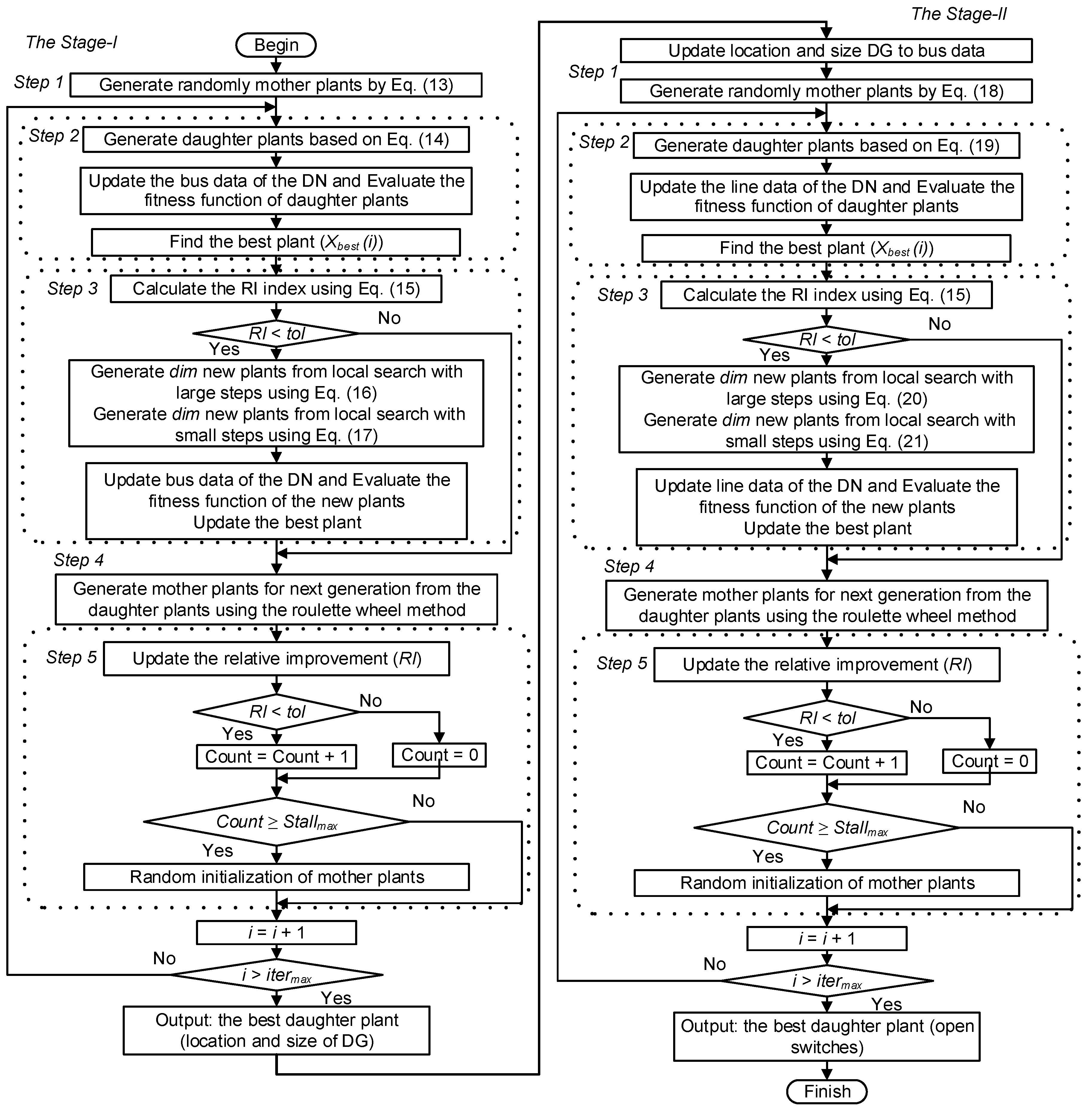
3. Runner Root Algorithm (RRA)

The RRA is a recently developed algorithm based on ideas from the plants bred via runners and roots [27]. In this work RRA has outperformed other algorithms via 25 benchmark functions. In RRA, two tools for exploitation is equipped consist of the roots mechanism and the elite selection mechanism. The former is designed to search around the best solution of current generation. The latter is designed to ensure the best solution of current generation is transferred to the next generation. For exploration, RRA is also equipped two tools consist of random jump of mother plants and re-initialization. In the former, each candidate solution is a random change to jump to any point in the search space. In the latter, the algorithm will be restarted after no considerable improvement in the fitness function after certain number of generations. Two tools equipped for exploitation and exploration mechanisms help RRA to be efficient at finding a global solution. In addition, in recently RRA has been applied for solving the network reconfiguration problem and it has demonstrated the advantages compared to other methods [28]. To implement the algorithm, reference [27] has used the following three rules:

—

The mother plants are generated the daughter plants in new locations through their runners to explore new resources.

—

The plants generate roots (runner) and root hairs (root) randomly to exploit new resources in new locations.

—

The daughter plants grows rapidly and produce more new plants at rich resources. Otherwise, if the daughter plants move toward poor resources, they will die.

Based on the three rules, the RRA method is implemented for optimizing of position and capacity of DGs considering network reconfiguration as follows.

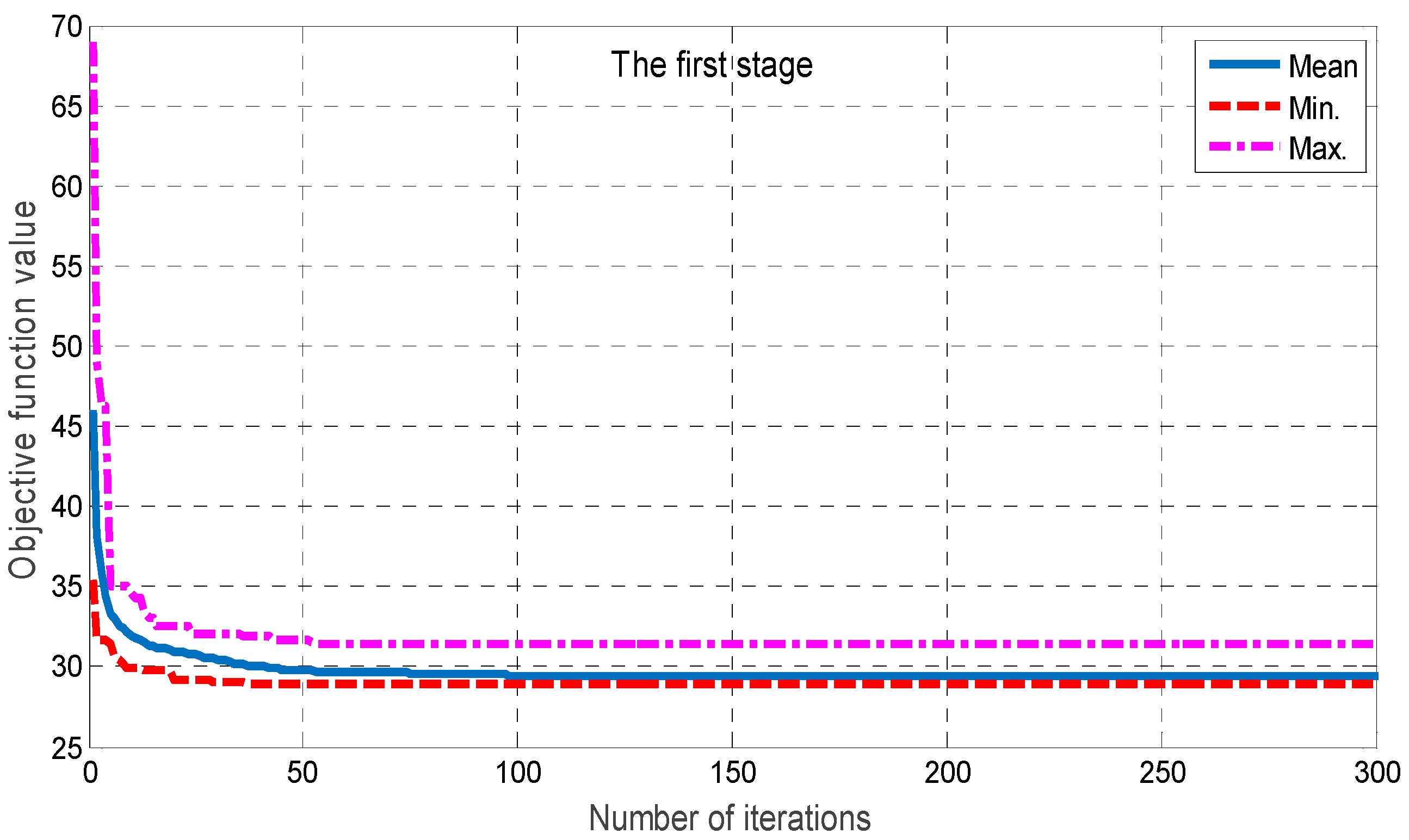
3.1. State-I: Optimizing of Position and Capacity of DGs in the Mesh Electric Distribution Network Using RRA

Step 1: Initialization

In the first stage, position and capacity of DGs is considered as a mother plant. Therefore, the mother plants are randomly initialized at the starting point of the algorithm as follows:

$${\mathrm{X}}_{mother,k}\left(\mathrm{i}\right)=\left\{round\left[2+rand\times \left({\mathrm{Lo}}_{max,d}-2\right)\right],P_{min,d}+rand\times (P_{max,d}-P_{min,d})\right\}$$

(13)

where $k=1,\dots ,N,i=1,\dots ,Ite{r}_{1,max}$ and $d=1,\dots ,ndg$.

From the population of mother plants which are location and the size of DGs, the bus data of the DN is updated, and the power flow is run by using the Newton–Raphson method to obtain power loss, node voltages and branch currents. Then, the value of the fitness function is calculated by using (9). The best plant (X_best ) of the population is determined.

Step 2: Generation of daughter plants

In this step, each daughter plant is generated by corresponding the mother plant. Noted that, the first plant is renewed by the best plant of the early generation. In the case of the first iteration, the first plant is the best mother plant of the randomly initialized population.

$$X_{daughter,k}\left(i\right)=\{\begin{array}{l}{X}_{best}\left(\mathrm{i}-1\right),k=1\\ X_{mother,k}\left(i\right)+d_{runner}\times rand,k=2,\dots ,N\end{array}$$

(14)

Then, the control variables represented for the location of DG are rounded to the integer values and the bus data of the DN is updated and the power flow is run by using the Newton–Raphson method to obtain power loss, node voltages and branch currents. The value of the fitness function is calculated by using (9). The best plant (X_best (i)) is determined again.

Step 3: Narrow search using big and small distance from the best plant

In step 3, if there are not a considerable improvement of the best plant in two iterations (i − 1)th and ith which is presented by a RI index, which is calculated by Equation (15). This step will be performed to generate new plants round the current best plant. Hence, the best plant is updated as follows:

$$X_{daughter,k}\left(i\right)=\{\begin{array}{l}{X}_{best}\left(\mathrm{i}-1\right),k=1\\ X_{mother,k}\left(i\right)+d_{runner}\times rand,k=2,\dots ,N\end{array}$$

(15)

where $f\left(X_{best}\left(i-1\right)\right)$ and $f\left(X_{best}\left(i\right)\right)$ are the fitness function value of the best plant in the generation (i − 1)th and the generation ith.

Narrow the search with large distance: in this procedure N_DG new plants are generated by adjusting the current best plant based on (16):

$$X_{perturbed,d}=round\left[vec\left\{1,1\dots ,1,1,1+d_{runner}\times ran{d}_d,1,\dots ,1\right\}\times X_{best}\left(i\right)\right]$$

(16)

where $d=1,\dots ,N_{DG}$; $vec\left\{1,1\dots ,1,1,1+d_{runner}\times rand,1,\dots ,1\right\}$ is a vector with the dth element is updated by $1+d_{runner}\times ran{d}_d$ and the remaining elements are equal to 1.

Narrow search with small distance: In this step, there are also N_DG new plants produced by using (17):

$$X_{perturbed,d}=round\left[vec\left\{1,1\dots ,1,1,1+d_{root}\times ran{d}_d,1,\dots ,1\right\}\times X_{best}\left(i\right)\right]$$

(17)

From the 2 × N_DG new daughter plants, the bus data of the DN is updated and the power flow is run by using the Newton–Raphson method to obtain the fitness function value based on (9). At the end of the step, the best solution (X_best (i)) is renewed again.

Step 4: Generation of new population of plants for next iteration

At the end step of each generation, the new mother plants for the next iteration are selected from the plants generated in step 3 based on the roulette wheel technique.

Step 5: Avoiding the local optimal solution

In this step, if there is not a considerable improvement of the best plant after the number of predefined iterations (stall_max), the RRA is restarted by generating random mother plants similar to step 1, otherwise it jumps to step 2.

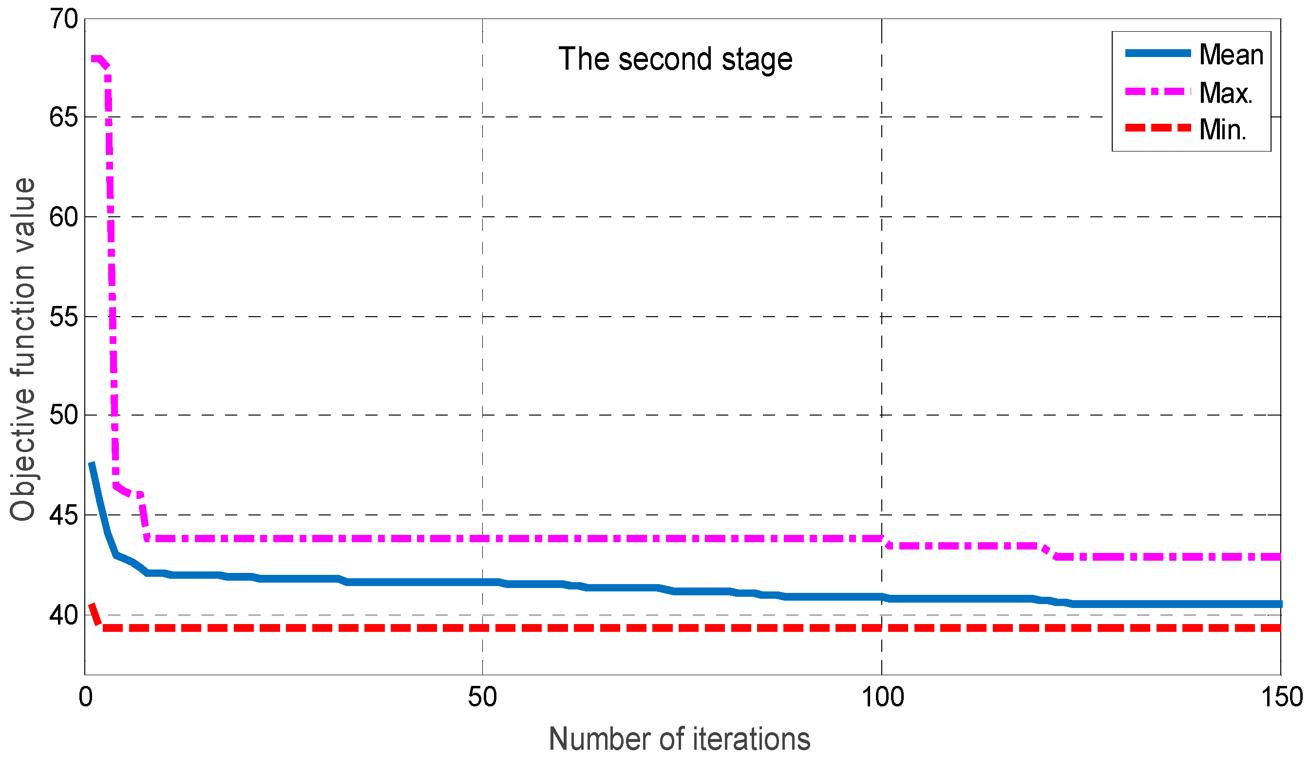
3.2. Stage-II: Network Reconfiguration after Installing Distributed Generators (DGs) Using RRA

In the second stage, each radial configuration of the DN which is presented by position of open switches. Therefore, the position of open switches is considered as a mother plant and the mother plants are randomly generated as follows:

$$X_{mother,k}\left(\mathrm{i}\right)=round\left[X_{low,d}+rand\times \left(X_{high,d}-X_{low,d}\right)\right]$$

(18)

where $d=1,\dots ,N_{SW}$, $X_{low,d}=1$ and $X_{high,d}$ is the number of switches in the mesh loop dth of the DN. Noted that each fundamental loop contains the number of switches that is formed by that loop.

Similar to the step 2 of the stage-I, each daughter plant is generated by corresponding the mother plant as (19). It is noticed that due to the daughter plant population being represented by open switches all of daughter plants are rounded to integer value. Then the line data of the DN is updated and the power flow is run to obtain the fitness function value based on (9). At the end of the step, the best solution (X_best (i)) is renewed again.

$$X_{daughter,k}\left(i\right)=\{\begin{array}{l}{X}_{best}\left(\mathrm{i}-1\right),k=1\\ round[X_{mother,k}\left(i\right)+d_{runner}\times rand],k=2,\dots ,N\end{array}$$

(19)

Similar to step 3 of state-I, in the second state, 2 × N_sw new plants are generated if this step will be performed by Equations (20) and (21). From Equations (20) and (21), it can be seen that all control variables are also rounded to the nearest integer to represent open switches.

$$X_{perturbed,d}=round\left[vec\left\{1,1\dots ,1,1,1+d_{runner}\times ran{d}_d,1,\dots ,1\right\}\times X_{best}\left(i\right)\right]$$

(20)

$$X_{perturbed,d}=round\left[vec\left\{1,1\dots ,1,1,1+d_{root}\times ran{d}_d,1,\dots ,1\right\}\times X_{best}\left(i\right)\right]$$

(21)

The step of production of mother plants for next iteration and step of escaping the local solution are definitely similar to them in the first stage. The flowchart of the proposed RRA for the problem of optimization of the position and capacity of DGs considering re-switching problem is presented in Figure 2.

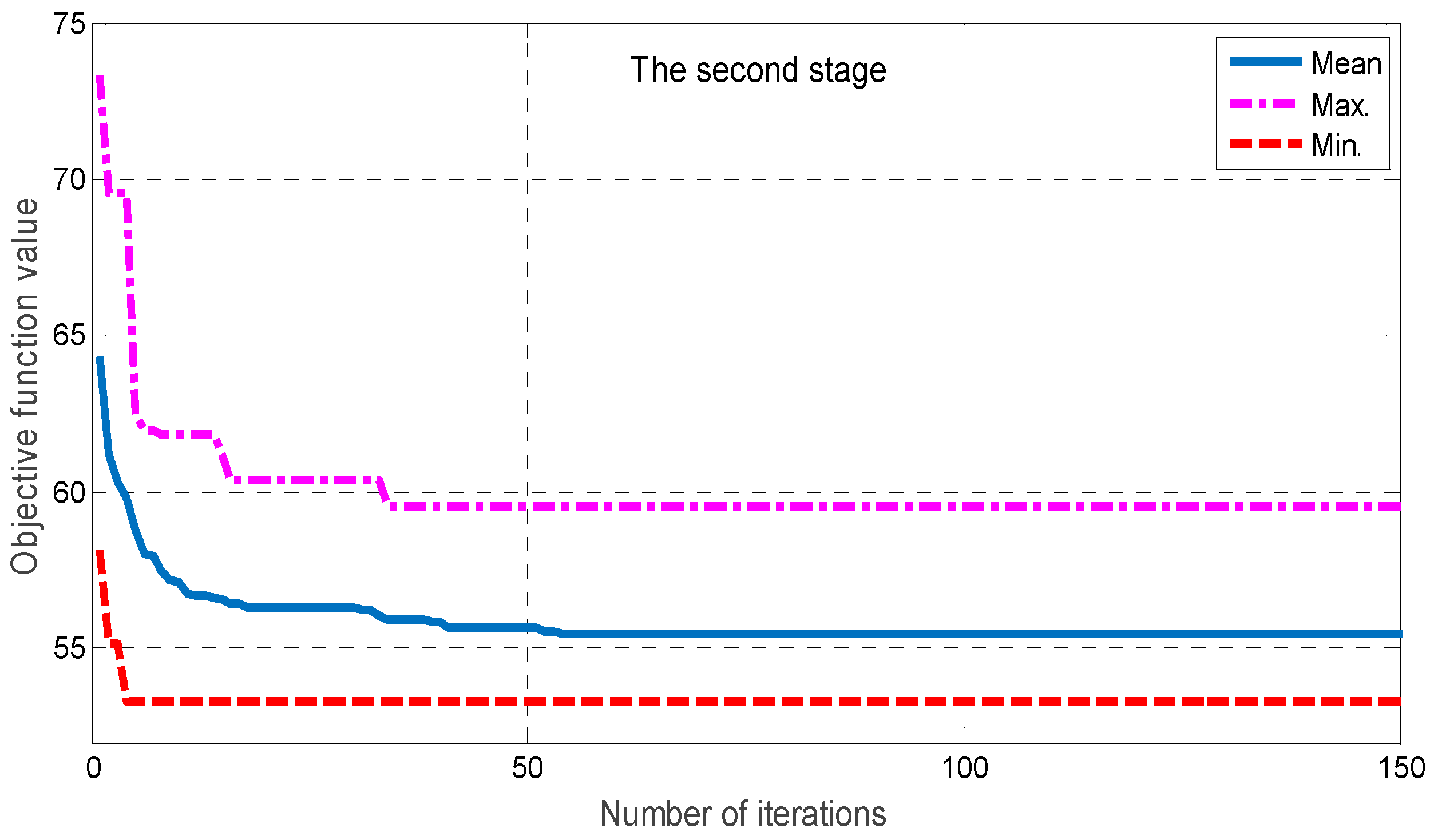
4. Numerical Results

The proposed method has been evaluated on two electric distribution networks including of 33 nodes and 69 nodes. In each system, three DGs with maximum capacity of 2 MW are installed. The proposed method is implemented in Matlab software on a personal computer with CPU Intel Core i3 4160 @ 3.6 GHz, 1 CPU, 8 GB, Windows 7 SP1 (64-bit). To show the superiority of the proposed method, the method of installation of DGs and reconfiguration of network simultaneously based on RRA is also implemented and compared with the proposed method using two states. The parameters of the RRA, which are determined by numerous trial executions and applied for two systems are presented in

Table 1. The parameters of the RRA for the 33 nodes and 69 nodes distribution network system.

System	The 33 and 69 Nodes
Item	State-I	State-II	Simultaneous
Mother plants	30	30	30
Maximum iterations	300	150	1000
Dimension	6	5	11
drunner	4	4	4
droot	2	2	2
stallmax	50	50	50

.

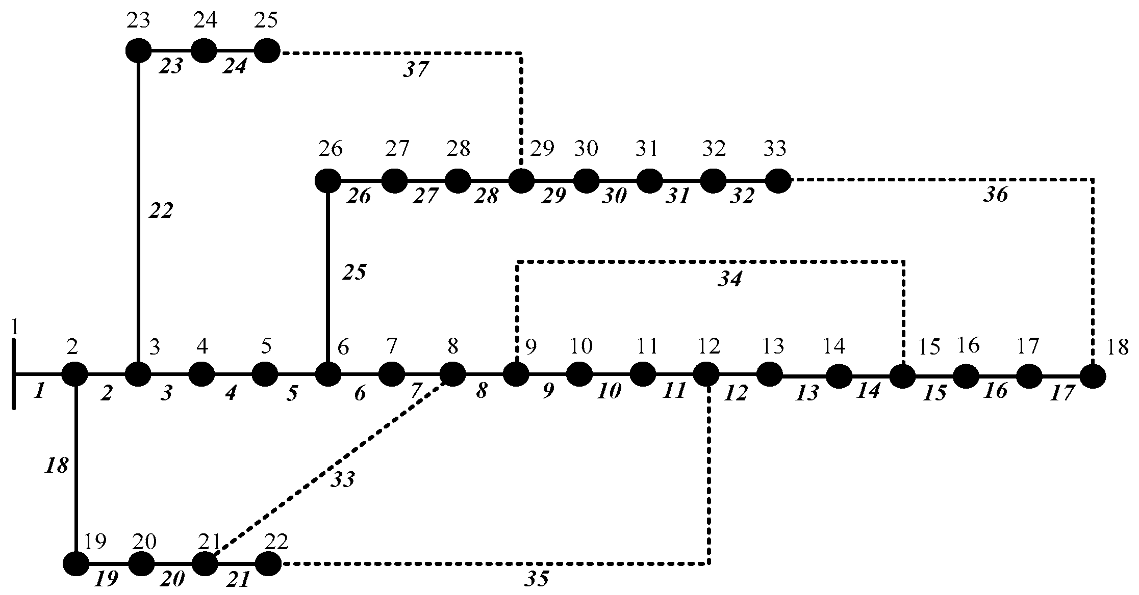
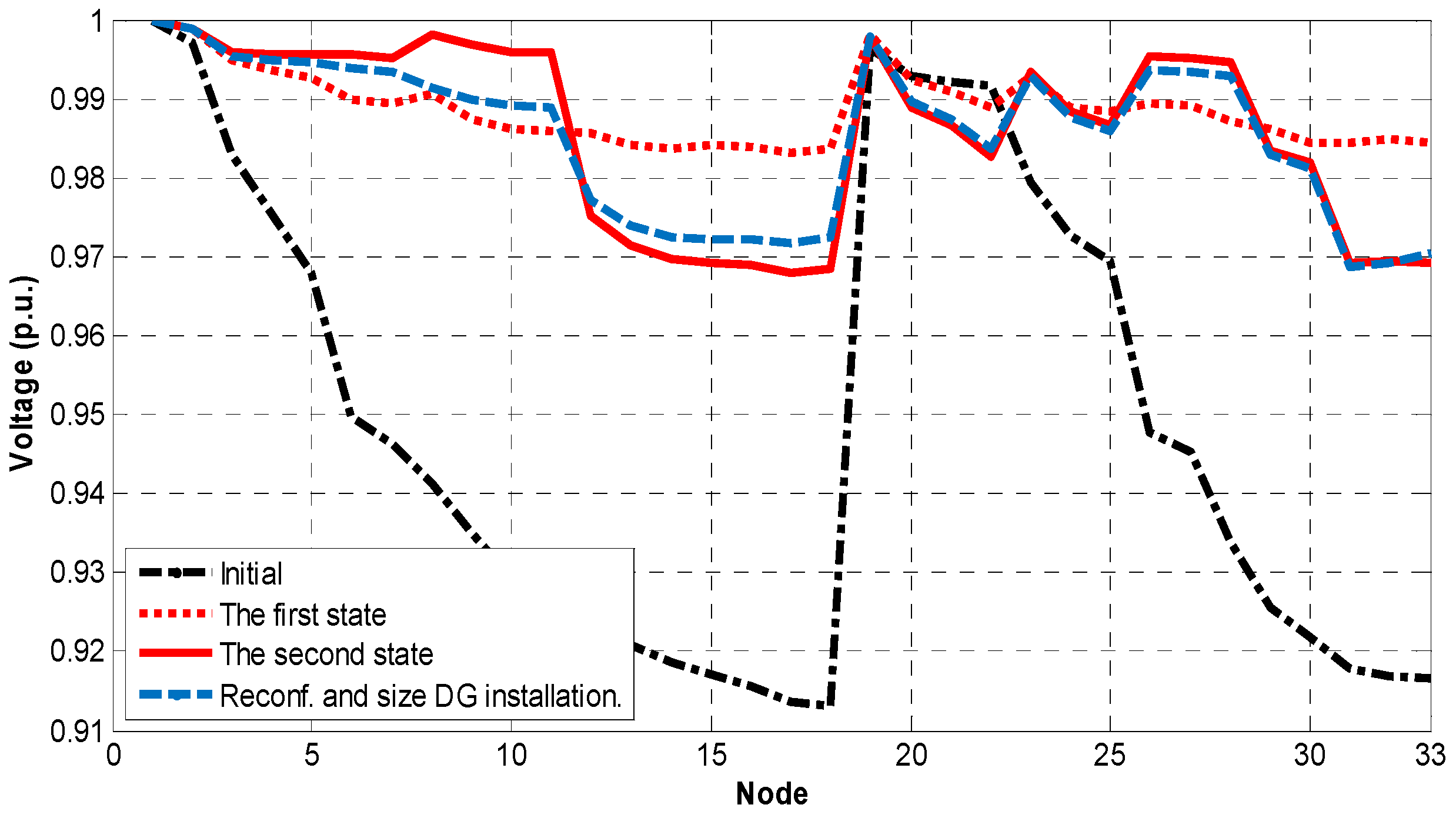
4.1. The 33 Nodes System

The 33 nodes system presented in Figure 3, consists 5 tie switches and 37 branches [29]. In a normal operation, switches {33, 34, 35, 36, and 37} are opened.

From

Table 2. Performance of the suggested technique on the 33-node system.

Item	Initial	Proposed Method Based on RRA		Simultaneous Rec. and DG Based on RRA
		State-I	State-II
Switches opened	33, 34, 35, 36, 37	None	33, 34, 11, 30, 28	33, 34, 11, 30, 28
Capacity of DG in MW (Bus number)	None	1.1326 (25), 0.8146 (32), 1.1011 (8)	1.1326 (25), 0.8146 (32), 1.1011 (8)	1.12095 (25), 0.87689 (18), 0.969711 (7)
Power loss (kW)	202.68	41.9051	53.3129	50.825
% Loss reduction	-	79.32	73.70	74.92
Max of fitness	-	46.2885	59.5526	64.0135
Mean of fitness	-	42.6949	55.4702	56.0123
Standard deviation (STD) of fitness	-	1.17681	2.50883	3.20373
CPU time (second)	-	25.0779	9.3156	80.7789
Average iterations	-	245.2	18.5	751.9

, power loss is decreased from 202.68 kW in the initial configuration to 41.9051 kW and 53.3129 kW using State-I and the State-II, respectively. The result from State-I shows that, the power loss is minimum because this is power loss caused by the mesh network. After using State-I to find the position and capacity of DGs in the mesh network, State-II is used to determine the open switches for radial operation, in which the open switches gained in the optimal configuration are {33, 34, 11, 30, 28}. So, the power loss is increased to 53.3129 kW compared with 41.9051 kW in State-I. However, compared with the method of simultaneous reconfiguration and placing DGs, these results are nearly the same as the results gained by the simultaneous reconfiguration and placing DGs method. The minimum power loss obtained by the simultaneous reconfiguration and placing DGs method is 50.825 kW which is only 2.4879 kW lower than the power loss caused by the optimum solution gained from the proposed method. In addition, the proposed method takes 34.39 seconds to execute the problem for both states, which is 46.39 seconds shorter than the simultaneous reconfiguration and placing DGs method. Moreover, it can be also be seen from Table 2 that the average values of the fitness function in State-I and State-II are closer the minimum value of the fitness function than that in the simultaneous reconfiguration and placing DGs method. This demonstrates that the proposed method also helps the RRA easily determine the optimal result for the problem.

The convergence behaviors for State-I and the State-II are presented Figure 4 and Figure 5. The voltage profiles of the initial, State-I, State-II and the simultaneous reconfiguration and placing DGs method are presented in Figure 6. As shown in the figure, the voltage magnitude at all nodes has been advanced after using the suggested method and the voltage profile of State-II is nearly the same with the voltage profile of the simultaneous reconfiguration and placing DGs method.

Comparison results with some of the methods are presented in

Table 3. Comparison of results on the 33-node system with the different methods.

Item	Proposed Method—RRA	CSA [13]	FWA [14]	HSA [15]	AWIDPSO [16]
Switches opened	33, 34, 11, 30, 28	33, 34, 11, 31, 28	7, 14, 11, 32, 28	7, 14, 10, 32, 28	7, 10, 13, 28, 32
Capacity of DG (in MW) (Bus number)	1.1326 (25), 0.8146 (32), 1.1011 (8)	0.8968 (18), 1.4381 (25), 0.9646 (7)	0.5367 (32), 0.6158 (29), 0.5315 (18)	0.5258 (32), 0.5586 (31), 0.5840 (33)	1.1215 (22), 1.3816 (23), 0.6425 (05)
Power loss (kW)	53.3129	53.21	67.11	73.05	52.15
% Loss reduction	73.70	73.75	66.89	63.95	74.27

. From the table, the loss reduction in percentage for the proposed method based on RRA is 0.05 higher than the result gained by CSA and 0.57 higher than the result gained by AWIDPSO, which is the method of solving the reconfiguration and simultaneous position and capacity of DGs. However, the performance of the proposed RRA is better than HSA and FWA. The percentage loss reduction for RRA, FWA and HSA is 73.70, 66.89 and 63.95, respectively. Note that the methods based on FWA and HSA have used different methods to pre-select the nodes for DGs installation on the initial radial network before optimization of the size of the DGs and reconfiguration.

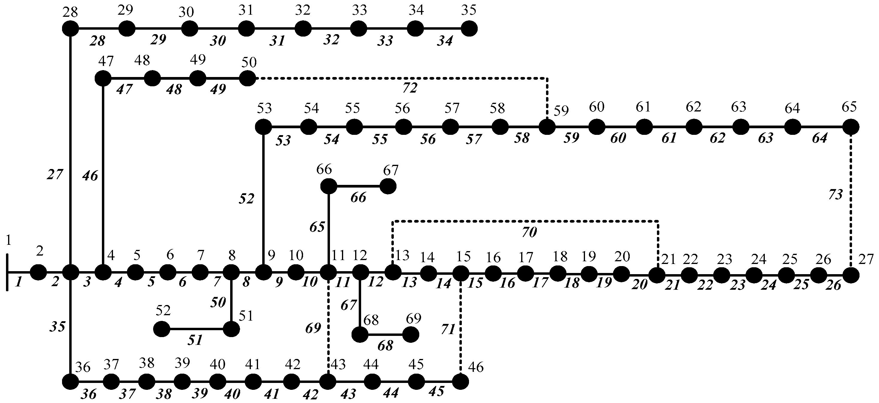
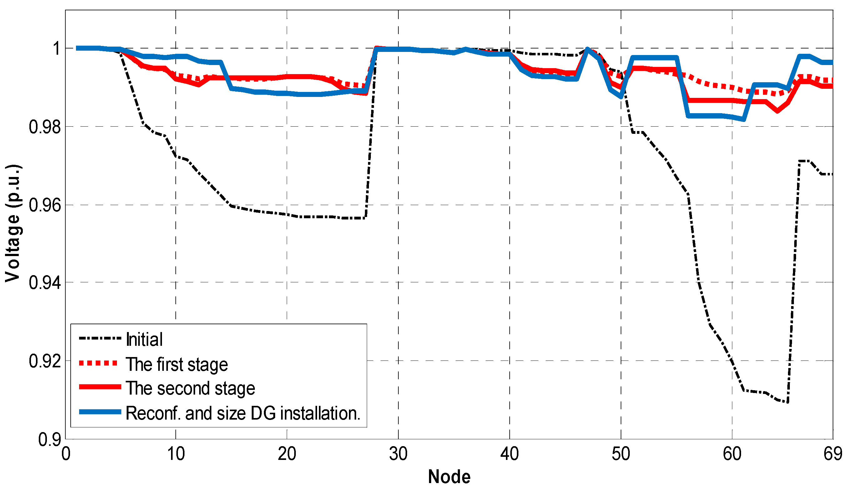
4.2. The 69 Nodes System

The 69 nodes distribution system shown in Figure 7 includes 73 branches and 5 tie switches [30]. The performance of the proposed approach on the 69 nodes system is presented in

Table 4. Performance of the suggested technique on the 69 nodes system.

Item	Initial	Proposed Method Based on RRA		Simultaneous Rec. and DGs Based on RRA
		State-I	State-II
Switches opened	69, 70, 71, 72, 73	None	69, 70, 12, 55, 63	69, 70, 14, 55, 61
Size of DG (in MW) (Bus number)	None	1.6175 (61), 0.7710 (50), 0.6752 (21)	1.6175 (61), 0.7710 (50), 0.6752 (21)	0.516112 (64), 1.45167 (61) 0.53696 (11)
Power loss (kW)	224.89	28.8875	39.31	35.1929
% Loss reduction	-	87.15	82.52	84.35
Max of fitness	-	31.3996	42.8777	48.622
Mean of fitness	-	29.3798	40.5443	40.3116
STD of fitness	-	0.7229	1.46845	3.25004
CPU time (second)	-	32.9654	27.2612	244.4863
Average iterations	-	240.15	71.05	807.15

.

From the table, in the initial configuration, power loss is 224.89 kW, which is decreased to 28.8875 kW, and 39.31 kW using State-I and the State-II, respectively. It can be seen that compared with the method of simultaneous reconfiguration and placing DGs, these results are nearly the same as the results gained by the simultaneous reconfiguration and placing DGs method. The minimum power loss obtained by the simultaneous reconfiguration and placing DGs method is 35.1929 kW which is only 4.1171 kW lower than the result obtained from the proposed method. In addition, in terms of CPU times, the proposed method takes 60.23 s to obtain the results for both states, which is 184.26 seconds lower than the simultaneous reconfiguration and placing DGs method. In addition, Table 4 show that the average values of the fitness function in State-I and the State-II are closer to the minimum value of the fitness function than that in the simultaneous reconfiguration and placing DGs method.

The convergence behaviors for State-I and State-II are presented Figure 8 and Figure 9. The voltage profiles of four cases are contrasted and shown in Figure 10. As illustrated in this figure, it is observed that the voltage magnitude at all nodes has been advanced after using the suggested method, and the voltage profile of State-II is nearly the same with the voltage profile of the simultaneous reconfiguration and placing DGs method.

Comparison results with FWA and HSA are presented in

Table 5. Comparison results on the 69 nodes system with the different methods.

Item	Proposed Method	CSA [13]	FWA [14]	HSA [15]
Switches opened	69, 70, 12, 55, 63	69, 70, 14, 58, 61	69, 70, 13, 55, 63	69, 17, 13, 58, 61
Size of DG (in MW) (Bus number)	1.6175 (61), 0.7710 (50), 0.6752 (21)	0.5413 (11), 0.5536 (65), 1.7240 (61)	1.1272 (61) 0.2750 (62) 0.4159 (65)	1.0666 (61) 0.3525 (60) 0.4257 (62)
Power loss (kW)	39.31	37.02	39.25	40.3
% Loss reduction	82.52	83.54	82.55	82.08

. The results showed that in the 69 nodes network system, the percentage loss reduction for RRA method is 1.02 higher than the result gained by CSA and these results are nearly to the same with the results gained by the FWA method with 82.55% and compared with HSA, it is better.

5. Conclusions

In this article, the method based on RRA has been successfully applied for optimizing the position and capacity of DGs taking into account reconfiguration of the network reconfiguration. The objective function is to minimize the power loss of the system. The main idea of the proposed method divided the problem into two states which consist of the optimization of the position and size of DGs on closed-loop distribution networks and the optimization of the operating structure of the DN after placing the DGs. In the both states, the RRA is used to determine the best solution. The calculated results show that the suggested method is capable of determining an optimal solution and is better than compared techniques in literature. The comparison results with the method of solving simultaneously the combined problem show that the power loss obtained from the proposed method is very close to that from the method of solving simultaneously the combined problem. Although the optimal results obtained by proposed method are slightly worse than those from method of solving simultaneously the combined problem but using the proposed method, the results of the location and size of the DG obtained, which is the design problem, are not affected by the results of the location of open switches on the DN, which is the operation problem. In addition, the calculated results have also shown that the proposed method can solve the problem faster compared with the method of reconfiguration and simultaneous position and capacity of DGs. Therefore, the suggested method is worthy of consideration for solving the position and capacity of DGs considering the network reconfiguration problem.

References

1. Hung, D.Q.; Mithulananthan, N.; Bansal, R.C. An optimal investment planning framework for multiple distributed generation units in industrial distribution systems. Appl. Energy 2014, 124, 62–72. [Google Scholar] [CrossRef] [Green Version]
2. Doagou-Mojarrad, H.; Gharehpetian, G.B.; Rastegar, H.; Olamaei, J. Optimal placement and sizing of DG (distributed generation) units in distribution networks by novel hybrid evolutionary algorithm. Energy 2013, 54, 129–138. [Google Scholar] [CrossRef]
3. Hung, D.Q.; Mithulananthan, N. Multiple distributed generator placement in primary distribution networks for loss reduction. IEEE Trans. Ind. Electron. 2013, 60, 1700–1708. [Google Scholar] [CrossRef]
4. Acharya, N.; Mahat, P.; Mithulananthan, N. An analytical approach for DG allocation in primary distribution network. Int. J. Electr. Power Energy Syst. 2006, 28, 669–678. [Google Scholar] [CrossRef]
5. Gözel, T.; Hocaoglu, M.H. An analytical method for the sizing and siting of distributed generators in radial systems. Electr. Power Syst. Res. 2009, 79, 912–918. [Google Scholar] [CrossRef]
6. Silvestri, A.; Berizzi, A.; Buonanno, S. Distributed generation planning using genetic algorithms. In Proceedings of the International Conference on PowerTech Budapest 99. (Cat. No.99EX376), Budapest, Hungary, 29 August–2 September 1999; p. 257. [Google Scholar]
7. Esmaeilian, H.R.; Fadaeinedjad, R. Energy Loss Minimization in Distribution Systems Utilizing an Enhanced Reconfiguration Method Integrating Distributed Generation. IEEE Syst. J. 2014, 9, 1430–1439. [Google Scholar] [CrossRef]
8. Kansal, S.; Kumar, V.; Tyagi, B. Optimal placement of different type of DG sources in distribution networks. Int. J. Electr. Power Energy Syst. 2013, 53, 752–760. [Google Scholar] [CrossRef]
9. Kayal, P.; Chanda, C.K. Placement of wind and solar based DGs in distribution system for power loss minimization and voltage stability improvement. Int. J. Electr. Power Energy Syst. 2013, 53, 795–809. [Google Scholar] [CrossRef]
10. Sedighizadeh, M.; Esmaili, M.; Esmaeili, M. Application of the hybrid Big Bang-Big Crunch algorithm to optimal reconfiguration and distributed generation power allocation in distribution systems. Energy 2014, 76, 920–930. [Google Scholar] [CrossRef]
11. Quadri, I.A.; Bhowmick, S.; Joshi, D. A hybrid teaching—Learning-based optimization technique for optimal DG sizing and placement in radial distribution systems. Soft Comput. 2018. [Google Scholar] [CrossRef]
12. Prabha, D.R.; Jayabarathi, T. Optimal placement and sizing of multiple distributed generating units in distribution networks by invasive weed optimization algorithm. Ain Shams Eng. J. 2016, 7, 683–694. [Google Scholar] [CrossRef]
13. Nguyen, T.T.; Truong, A.V.; Phung, T.A. A novel method based on adaptive cuckoo search for optimal network reconfiguration and distributed generation allocation in distribution network. Int. J. Electr. Power Energy Syst. 2016, 78, 801–815. [Google Scholar] [CrossRef]
14. Mohamed Imran, A.; Kowsalya, M.; Kothari, D.P. A novel integration technique for optimal network reconfiguration and distributed generation placement in power distribution networks. Int. J. Electr. Power Energy Syst. 2014, 63, 461–472. [Google Scholar] [CrossRef]
15. Rao, R.S.; Ravindra, K.; Satish, K.; Narasimham, S.V.L. Power Loss Minimization in Distribution System Using Network Reconfiguration in the Presence of Distributed Generation. IEEE Trans. Power Syst. 2013, 28, 1–9. [Google Scholar] [CrossRef]
16. Subramaniyan, M.; Subramaniyan, S.; Veeraswamy, M.; Jawalkar, V.R. Optimal reconfiguration/distributed generation integration in distribution system using adaptive weighted improved discrete particle swarm optimization. COMPEL-Int. J. Comput. Math. Electr. Electron. Eng. 2018. [Google Scholar] [CrossRef]
17. Nguyen, T.T.; Truong, A.V. Distribution network reconfiguration for power loss minimization and voltage profile improvement using cuckoo search algorithm. Int. J. Electr. Power Energy Syst. 2015, 68, 233–242. [Google Scholar] [CrossRef]
18. Merlin, A.; Back, H. Search for a minimal loss operating spanning tree configuration in an urban power distribution system. In Proceedings of the 5th power Syst. Computation conference (PSCC), Cambridge, UK, 1–5 September 1975; pp. 1–18. [Google Scholar]
19. Civanlar, S.; Grainger, J.J.; Yin, H.; Lee, S.S.H. Distribution feeder reconfiguration for loss reduction. IEEE Trans. Power Deliv. 1988, 3, 1217–1223. [Google Scholar] [CrossRef]
20. Duan, D.L.; Ling, X.D.; Wu, X.Y.; Zhong, B. Reconfiguration of distribution network for loss reduction and reliability improvement based on an enhanced genetic algorithm. Int. J. Electr. Power Energy Syst. 2015, 64, 88–95. [Google Scholar] [CrossRef]
21. Esmaeilian, H.R.; Fadaeinedjad, R. Distribution system efficiency improvement using network reconfiguration and capacitor allocation. Int. J. Electr. Power Energy Syst. 2015, 64, 457–468. [Google Scholar] [CrossRef]
22. Teimourzadeh, S.; Zare, K. Application of binary group search optimization to distribution network reconfiguration. Int. J. Electr. Power Energy Syst. 2014, 62, 461–468. [Google Scholar] [CrossRef]
23. Mohamed Imran, A.; Kowsalya, M. A new power system reconfiguration scheme for power loss minimization and voltage profile enhancement using Fireworks Algorithm. Int. J. Electr. Power Energy Syst. 2014, 62, 312–322. [Google Scholar] [CrossRef]
24. Arandian, B.; Hooshmand, R.; Gholipour, E. Decreasing activity cost of a distribution system company by reconfiguration and power generation control of DGs based on shuffled frog leaping algorithm. Int. J. Electr. Power Energy Syst. 2014, 61, 48–55. [Google Scholar] [CrossRef]
25. Haghifam, M.R.; Olamaei, J.; Andervazh, M.R. Adaptive multi-objective distribution network reconfiguration using multi-objective discrete particles swarm optimisation algorithm and graph theory. IET Gener. Transm. Distrib. 2013, 7, 1367–1382. [Google Scholar]
26. Swarnkar, A.; Gupta, N.; Niazi, K.R. Adapted ant colony optimization for efficient reconfiguration of balanced and unbalanced distribution systems for loss minimization. Swarm Evol. Comput. 2011, 1, 129–137. [Google Scholar] [CrossRef]
27. Merrikh-Bayat, F. The runner-root algorithm: A metaheuristic for solving unimodal and multimodal optimization problems inspired by runners and roots of plants in nature. Appl. Soft Comput. 2015, 33, 292–303. [Google Scholar] [CrossRef]
28. Nguyen, T.T.; Nguyen, T.T.; Truong, A.V.; Nguyen, Q.T.; Phung, T.A. Multi-objective electric distribution network reconfiguration solution using runner-root algorithm. Appl. Soft Comput. 2017, 52, 93–108. [Google Scholar] [CrossRef]
29. Baran, M.E.; Wu, F.F. Network reconfiguration in distribution systems for loss reduction and load balancing. IEEE Trans. Power Deliv. 1989, 4, 1401–1407. [Google Scholar] [CrossRef]
30. Chiang, H.D.; Jean-Jumeau, R. Optimal network reconfigurations in distribution systems: Part 2: Solution algorithms and numerical results. IEEE Trans. Power Deliv. 1990, 5, 1568–1574. [Google Scholar] [CrossRef]
Figure 1. One loop distribution network.
Energies 12 00106 g001
Figure 2. The flowchart for determining the position and capacity of distributed generators (DGs) in the mesh electric distribution considering re-switching problem based on the runner root algorithm (RRA) method.
Energies 12 00106 g002
Figure 3. The 33 nodes distribution system.
Energies 12 00106 g003
Figure 4. The convergence of RRA in the first stage over 50 independent runs for the 33-node system.
Energies 12 00106 g004
Figure 5. The convergence of RRA in the second stage over 50 independent runs for the 33-node system.
Energies 12 00106 g005
Figure 6. Voltage profiles in four cases of the 33-node system.
Energies 12 00106 g006
Figure 7. The 69 nodes distribution system.
Energies 12 00106 g007
Figure 8. The convergence of RRA in the first stage over 50 independent runs for the 69-node test system.
Energies 12 00106 g008
Figure 9. The convergence of RRA in the second stage over 50 independent runs for the 69-node test system.
Energies 12 00106 g009
Figure 10. Voltage profiles in four cases of the 69 nodes system.
Energies 12 00106 g010