Impacts of Load Profiles on the Optimization of Power Management of a Green Building Employing Fuel Cells


Department of Mechanical Engineering, National Taiwan University, Taipei 10617, Taiwan
*
Author to whom correspondence should be addressed.
Energies 2019, 12(1), 57; https://doi.org/10.3390/en12010057
Submission received: 25 October 2018
/
Revised: 12 December 2018
/
Accepted: 24 December 2018
/
Published: 25 December 2018
(This article belongs to the Special Issue Short-Term Load Forecasting by Artificial Intelligent Technologies)
Abstract
:This paper discusses the performance improvement of a green building by optimization procedures and the influences of load characteristics on optimization. The green building is equipped with a self-sustained hybrid power system consisting of solar cells, wind turbines, batteries, proton exchange membrane fuel cell (PEMFC), electrolyzer, and power electronic devices. We develop a simulation model using the Matlab/SimPowerSystemTM and tune the model parameters based on experimental responses, so that we can predict and analyze system responses without conducting extensive experiments. Three performance indexes are then defined to optimize the design of the hybrid system for three typical load profiles: the household, the laboratory, and the office loads. The results indicate that the total system cost was reduced by 38.9%, 40% and 28.6% for the household, laboratory and office loads, respectively, while the system reliability was improved by 4.89%, 24.42% and 5.08%. That is, the component sizes and power management strategies could greatly improve system cost and reliability, while the performance improvement can be greatly influenced by the characteristics of the load profiles. A safety index is applied to evaluate the sustainability of the hybrid power system under extreme weather conditions. We further discuss two methods for improving the system safety: the use of sub-optimal settings or the additional chemical hydride. Adding 20 kg of NaBH4 can provide 63 kWh and increase system safety by 3.33, 2.10, and 2.90 days for the household, laboratory and office loads, respectively. In future, the proposed method can be applied to explore the potential benefits when constructing customized hybrid power systems.
1. Introduction
Today’s energy crises and pollution problems have increased the current interest in fuel cell research. One of the most popular fuel cells is the proton exchange membrane fuel cell (PEMFC), which can transform chemical energy into electrical energy with high energy conversion efficiency by electrochemical reactions. At the anode, the hydrogen molecule ionizes, releasing electrons and H+ protons. At the cathode, oxygen reacts with electrons and H+ protons through the membrane to form water. The electrons pass through an electrical circuit to create current output of the PEMFC. The PEMFC has several advantageous properties, including a low operating temperature and high efficiency. However, it also has very complex electrochemical reactions, so attempts to develop dynamic models for PEMFC systems have become an active research focus. For example, Ceraolo et al. [1] developed a PEMFC model that contained the Nernst equation, the cathodic kinetics equation, and the cathodic gas diffusion equation. Similarly, Gorgun [2] presented a dynamic PEMFC model that included water phenomena, electro-osmotic drag and diffusion, and a voltage ancillary. These models have served as the basis of many advanced control techniques aimed at improving the performance of PEMFC systems. For instance, Woo and Benziger [3] tried to improve PEMFC efficiency using a proportional-integral-derivative (PID) controller to regulate the hydrogen flow rate. Vega-Leal et al. [4] controlled the air and hydrogen flow rates to optimize the PEMFC output power. Park et al. [5] considered load perturbations and applied a sliding mode control to maintain the pressures of hydrogen and oxygen regardless of current changes. Wang et al. [6] designed a robust controller to regulate the air flow rate to ensure that the PEMFC provided a steady output voltage. This idea was further extended to a multi-input multi-output (MIMO) PEMFC model to reduce hydrogen consumption while providing a steady voltage [7]. Reduced-order robust control [8] and robust PID control [9] were also proposed for hardware simplification and industrial applications.
A PEMFC can supply sustainable power as long as the hydrogen supply is continuous; therefore, the PEMFC has been widely applied in transportation [10,11,12,13,14,15,16,17,18,19] and stationary power systems [20,21,22,23,24,25,26,27,28,29]. A PEMFC can also supply sustainable energy regardless of weather conditions, making it a reliable power source when solar and wind energy are unavailable. However, the price of hydrogen energy is generally high when compared to other green (e.g., solar) energy, so the PEMFC is typically integrated with other energy sources and storage systems to form hybrid power systems. For example, Zervas et al. [30] presented a hybrid system that contained photovoltaics (PV), a PEMFC, and an electrolyzer with metal hydride tanks. Rekioua et al. [31] considered a hybrid photovoltaic-electrolyzer-fuel cell system and discussed its optimization by selection of different topologies. Nizetic et al. [29] proposed a system for household application that used a high-temperature PEMFC to drive a modified heat pump system, with a cost of less than 0.16 euro/kWh.
The role of the PEMFC in hybrid power systems is unique, because it can act as both an energy source and an energy storage system. It serves as an energy source to provide backup power when the load requirement is greater than the energy supply from other energy sources and as an energy storage system to store hydrogen electrolyzed by redundant energy when the energy supply is greater than the consumption [32]. Some hybrid power systems have recently been implemented in practice. For instance, Singh et al. [22] presented a PEMFC/PV hybrid system for stand-alone applications in India. Das et al. [23] introduced the PV/battery/PEMFC and PV/battery systems installed in Malaysia. Al-Sharafi et al. [24] considered six different systems in the Kingdom of Saudi Arabia. Martinez-Lucas et al. [25] demonstrated a system based on wind turbine (WT) and pump storage hydropower on the Canary Island of El Hierro, Spain. Kazem et al. [27] evaluated four different hybrid power systems on Masirah Island, Oman.
Because of the influence of weather conditions and loads, the costs of these hybrid systems can be optimized by changing the system configurations. For example, Ettihir et al. [26] applied the adaptive recursive least square method to find the best efficiency and power operating points. Singh et al. [22] applied a fuzzy logic program to calculate system costs and concluded that the PEMFC and battery are the most significant modules for meeting load demands late at night and in the early morning. Kazem et al. [27] showed that that a PV/WT/battery/diesel hybrid system had the lowest cost for energy production. Cozzolino et al. [28] analyzed the Tunisia and Italy (TUNeIT) Project and showed that this almost self-sustaining renewable power plant, consisting of a WT, PV, battery, PEMFC, and diesel engine, ran at a cost of 0.522 €/kWh. Wang et al. [33] studied a hybrid system that consisted of a WT, PV, battery, and an electrolyzer and concluded that the costs and reliability of hybrid power systems can be greatly improved by adjusting the component sizes. They also showed that power management can help to reduce system costs [32]. The present paper extends these ideas by discussing the impacts of load profiles on the optimization of system costs. We applied three typical load profiles to a hybrid system and discussed the cost and energy distribution. We also evaluated the guaranteed operation durations (called system safety) of hybrid systems and discussed the applications of two methods to extend system safety.
The remainder of this paper is arranged as follows: Section 2 introduces the green building and its hybrid power system. Based on the system characteristics, we build a general hybrid power model consisting of solar cells, WTs, batteries, a PEMFC, hydrogen electrolysis, and chemical hydrogen generation. The model parameters were tuned based on experimental data to allow the prediction of system responses under different operation conditions. Historical irradiation and wind data were applied to estimate the power supplied by the PV and WT, while three typical load profiles were considered to understand their impacts on system optimization. Section 3 defines three performance indexes for evaluating hybrid power systems equipped with different components and management strategies. We applied three typical loads to optimize system design by tuning the component sizes and power management. The results showed that the optimization processes can effectively reduce the energy costs by 38.9%, 40.0%, and 28.6% and greatly improve system reliability by 4.89%, 26.42%, and 5.08% for household, laboratory, and office loads, respectively. The guaranteed sustainable operation periods under extreme weather conditions were also estimated. The results revealed that system sustainability can be improved by the use of a sub-optimal design or chemical hydrides. We also discuss the critical prices of implementing a chemical hydrogen generation system. Conclusions are then drawn in Section 4.
2. System Description and Modelling
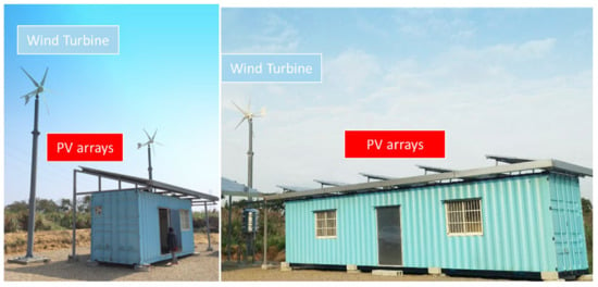
The green building, as shown in Figure 1 [34], is located in Miao-Li County in Taiwan. It was constructed by China Engineering Consultants Inc. (CECI) and was equipped with a hybrid power system that consisted of 10 kW PV arrays, 6 kW WTs, 800Ah lead-acid batteries, a 3 kW PEMFC, and a 2.5 kW electrolyzer with a hydrogen production rate of 500 L/h. The building was autonomous and did not connect to the main grid, i.e., its electricity was supplied completely by green energy, such as solar and wind. The energy can be stored for use when the green energy is less than the load demands. These components were originally selected to provide a daily energy supply of about 20 kWh based on the National Aeronautics and Space Administration (NASA) data [34], as illustrated in Table 1. Solar energy was abundant in the summer but poor in the winter, so wind energy was expected to compensate for solar energy in the winter. However, Chen and Wang [32] applied the Vantage Pro2 Plus Stations [35] to measure the real weather data on the building site and found that the wind energy was not sufficient to compensate for the reduced solar energy in the winter. Further analyses of the energy costs also revealed that the wind energy was not economically efficient for this building, as illustrated in Table 2. Therefore, the following component selection principles were suggested to improve system performance [32]:
- (1)
- Energy sources: the use of PV and PEMFC in the green building was suggested, because solar energy was the most economical energy source and the PEMFC could guarantee energy sustainability. The PEMFC can be regarded as an energy source that provides steady energy and as an energy storage system when coupled with a hydrogen electrolyzer. Considering the transportation, storage, and efficiency of energy conversion, the PEMFC with chemical hydrogen generation by NaBH4 [36] was suggested for the system.
- (2)
- Energy storage: the lead-acid battery was suggested because of its greater than 90% efficiency [37]. Though the PEMFC with a hydrogen electrolyzer can also store energy, the conversion efficiency from electricity into hydrogen was only about 60% [33]. Therefore, the total energy storage efficiency was about 36%, because the PEMFC converted hydrogen into electricity with an efficiency of about 60% [38]. Note that the LiFe battery has a higher efficiency (more than 95%) but is much more expensive than a lead-acid battery. Therefore, the lead-acid battery was preferred for the green building.
That is, the selection of multiple energy sources and storages depended on the local conditions and load requirements.
2.1. The Hybrid Power Model
A general hybrid power model, as shown in Figure 2, was developed to evaluate system performance at different operating conditions (e.g., varying the component sizes and power management strategies) [32,33,39]. The model consisted of a PV module, a WT module, a battery module, a PEMFC module, an electrolyzer module, a chemical hydrogen generation module, and a load module. The power management strategies were applied to operate these modules based on battery state-of-charge (SOC). The module parameters were adjusted by the component characteristics and experimental responses to allow prediction and analysis of the system dynamics without the need for extensive experiments [39,40].
First, the 1 kW PV module was developed based on the following equation [32,41]:
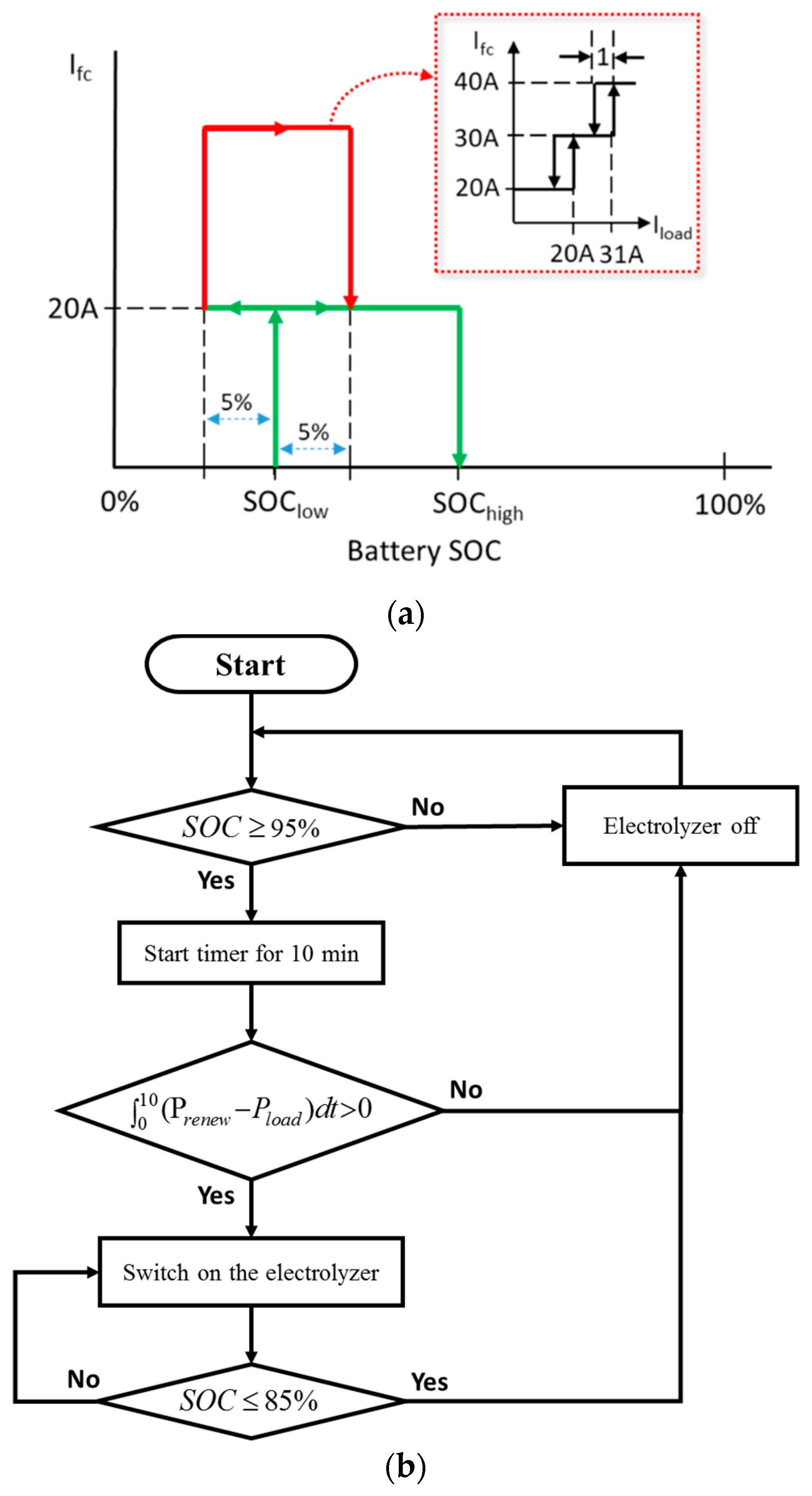
where PPV (Watt) and E (Watt per meter square) represent solar power and irradiance, respectively. Second, the WT module was presented as a look-up table, according to the relation between wind power and wind speed [33,42]. Third, the PEMFC acted as a back-up power source to guarantee system sustainability based on the following management strategies (see Figure 3a) [39]:
- (1)
- When the battery SOC dropped to the lower bound, SOClow, the PEMFC was switched on to provide a default current of 20 A at the highest energy efficiency [41].
- (2)
- When the SOC continuously dropped to SOClow − 5%, the PEMFC current was increased according to the required load until the SOC was raised to SOClow + 5%, where the PEMFC provided a default current of 20 A.
- (3)
- When the battery SOC reached SOChigh, the PEMFC was switched off.
Therefore, the power management can be adjusted by tuning SOClow and SOChigh. As a last stage, the hydrogen electrolyzer transferred redundant energy to hydrogen storage based on the following strategies (see Figure 3b) [33]:
- (1)
- When the battery SOC was higher than 95%, the extra renewable energy was regarded as redundant.
- (2)
- The electrolyzer module would wait for ten minutes to avoid chattering. If the total redundant energy increased during this period, the electrolyzer was switched on.
- (3)
- When the hydrogen tank was full or the battery SOC dropped to 85%, the electrolyzer was switched off.
Thus, the electrolyzer produced hydrogen when the battery SOC was between 85% and 95%. The electrolyzer module was set to produce hydrogen at a rate of 1.14 L/min by consuming a constant power of 410 W, based on the experimental results [33].
2.2. Inputs Energy and Output Loads
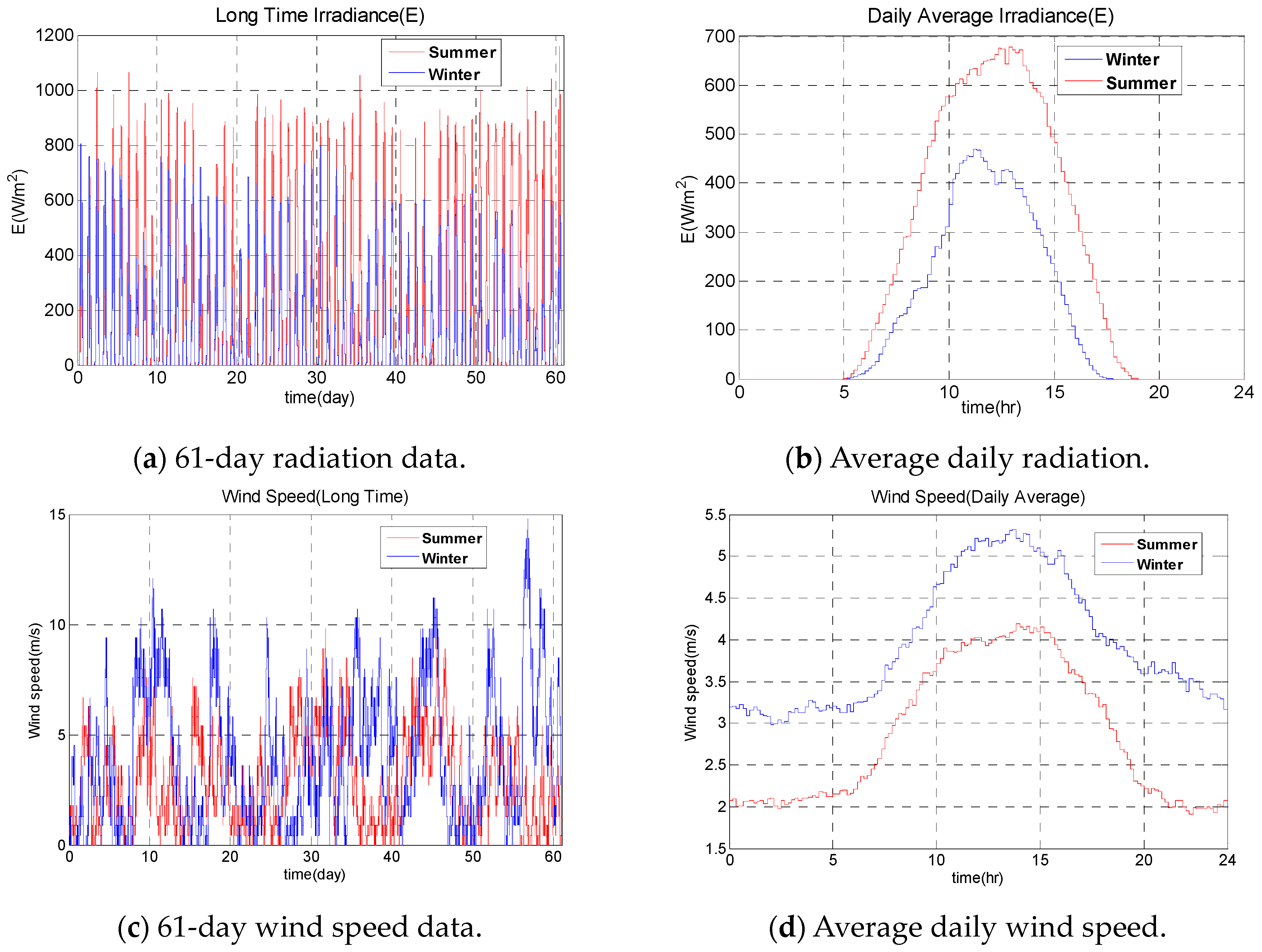
We applied the historical irradiation and wind speed data [32], as shown in Figure 4, to the PV and WT modules, respectively. As shown in Figure 4, solar radiation was abundant in the summer but poor in the winter; therefore, solar energy in the summer can be stored for use in the winter. Conversely, the wind speed was high in the winter but low in the summer, so wind energy was expected to compensate for the lack of solar energy in the winter. However, the compensation effects were not as significant as originally designed because the wind was not sufficiently strong and the energy cost was much higher (see Table 2) when compared to other energy sources. Note that both solar and wind energy were concentrated in the daytime, indicating that this energy should be stored for use at night.
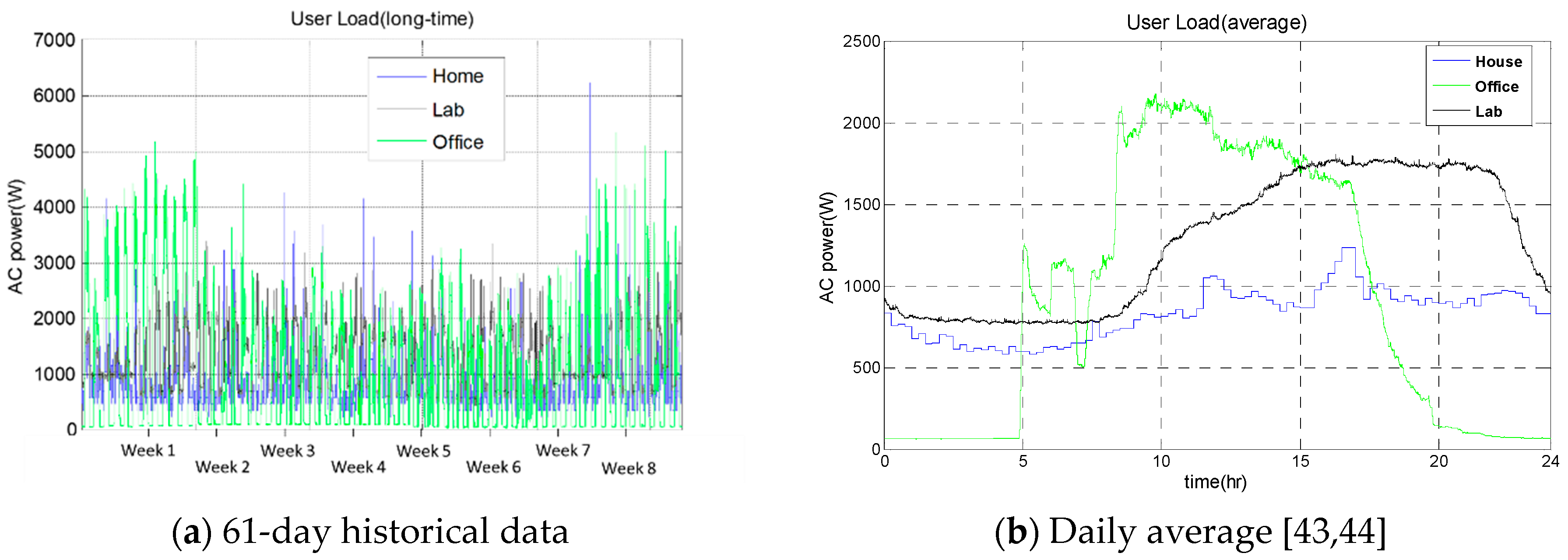
Three standard load profiles [43,44], as illustrated in Figure 5, were applied to the load module to investigate the impacts of loads on the optimization of the hybrid power system. The 61-day historical data were used for simulation and optimization analyses. Table 3 illustrates the statistical data of these load profiles, where the household had the largest historically peak and the office had the largest daily average peak, while the laboratory load had the greatest energy consumption. Therefore, we used these three typical loads to demonstrate how load characteristics can affect the performance optimization of the hybrid power system.
3. Design Optimization of the Hybrid Power System
The hybrid power model was applied to predict system responses under different conditions, such as the use of varying components and loads. We defined three indexes to evaluate the performance of the hybrid power system: cost, reliability, and safety, as described by the following:
(1) System cost: the system cost J(b, s, w) consisted of two parts, Ji and Jo, as follows [39]:
where Ji and Jo indicate the initial and operation costs, respectively. The subscripts b, s, and w represent the numbers of batteries, PV arrays, and WTs in units of 100Ah, 1kW, and 3kW, respectively. The initial cost Ji accounted for the investment in the components, such as the PEMFC, power electric devices, PV arrays, WT, hydrogen electrolyzer, chemical hydrogen generator, and battery set, as follows:
where k = PEMFC, DC, solar, WT, HE, CHG, and batt, respectively.
J(b, s, w) = Ji(b, s, w) + Jo(b, s, w)
The operation cost Jo included the hydrogen consumption and the maintenance of the WT and PV arrays, as in the following:
where l = NaBH4, WT, and solar, respectively.
We calculated the initial costs and the operation costs as follows:
in which C and n are the price per unit and the installed units, respectively, for each component k. CRF represented the capital recovery factor that was defined as [32,33,39]:
where ir is the inflation rate, which was set as 1.26% in this paper by referring to the average annual change of consumer price index of Taiwan [39], and ny is the expected life of the components. The price and expected life of the components are illustrated in Table 4 were used to calculate the system costs in the following examples.
(2) System reliability: the reliability of the hybrid system was defined as the loss of power supply (LPSP) as follows [32,33,39]:
in which LPS(t) was the shortage (lost) of power supply at time t, while P(t) was the power demand of the load profile at time t. Therefore, indicated the insufficient energy supply and represented the total energy demand for the entire simulation. If the power supply met the load demand at all times, (i.e., LPS(t) = 0, ), then the system was completely reliable with LPSP = 0.
(3) System safety: system safety was defined as the guaranteed sustainable period of the hybrid power system under extreme weather conditions when no solar or wind energy was available. Suppose the energy stored in the system was Estore and the average daily energy consumption was Eday; then, the system safety can be defined as follows:
For example, average daily energy demand is 19.96, 30.41, and 22.32 kWh for the household, laboratory, and office, respectively (see Table 3). Therefore, if the energy stored in the battery and hydrogen is 60 kWh, the system safety is 3.01, 1.97, and 2.69 days for the laboratory, office, and household, respectively. When considering the efficiency of the battery and inverter both as 90%, then the system safety is 2.70, 1.78, and 2.42 days, respectively.
We applied the three typical loads to investigate their impacts on the optimization of the hybrid power system by tuning the component sizes and power management strategies.
3.1. Household Load
Applying the household load (see Figure 5) to the original system layout (b, s, w) = (8, 10, 2) and management settings of (SOClow, SOChigh) = (40%, 50%) gave the system’s reference plot shown in Figure 6a, where the system cost was estimated as J = 1.300 $/kWh with LPSP = 4.89% (see Step 1 of Table 5). From Figure 6a, the system cost can be reduced to J = 1.169 $/kWh by adjusting the components as (b, s, w) = (18, 9, 2) but with a possible power cut (LPSP = 2.61%, see Step 2 of Table 5). If the requirement was LPSP = 0, then the optimal system cost was J = 1.189 $/kWh, achieved by setting (b, s, w) = (18, 10, 2) (see Step 3 of Table 5). That is, we can reduce the system cost from J = 1.300 to 1.189 $/kWh, while improving the system reliability from LPSP = 4.89% to 0.
Because the cost of wind energy was much higher than the cost of solar energy (see Table 2) and the compensation effects were not significant (see Figure 4), the use of solar and a PEMFC with chemical hydrogen production was viewed as economically efficient for the green building [32]. Therefore, we set w = 0 and the resulting optimization showed that the system cost can be significantly reduced to J = 0.822 $/kWh by setting (b, s, w) = (15, 15, 0), as illustrated in Step 4 of Table 5. Furthermore, when we fixed the component settings of (b, s, w) = (15, 15, 0) and tuned the power management strategies (SOClow, SOChigh) = (30%, 40%), the system cost was further decreased to J = 0.810 $/kWh (see Step 5 of Table 5). Steps 6 and 7 illustrate the iterative tuning of component size and power management, respectively. The results indicated that the system cost converged to J = 0.794 $/kWh with (b, s, w) = (23, 15, 0) and (SOClow, SOChigh) = (30%, 40%). Compared with the original cost, the cost was reduced by 38.9%, while maintaining complete system reliability. Note that the iterative method can greatly reduce the computation time because the simultaneous optimization of four parameters (b, s, SOClow, SOChigh) took much longer than iterative optimization, as indicated in [45]. Therefore, the proposed iterative optimization can be applied for a quick estimation of the system behavior. Simultaneous optimization can be considered for potentially better optimization if time permits.
3.2. Laboratory Load
Similarly, the results of applying the laboratory load (see Figure 5) to the hybrid power model are shown in Figure 7 and Table 6. First, the original system layout (b, s, w) = (8, 10, 2) with management settings of (SOClow, SOChigh) = (40%, 50%) resulted in a system cost of J = 1.100 $/kWh and LPSP = 26.42%. Note that the LSPS was much higher than was obtained for the household, because the laboratory load was mainly at night and the stored energy by hydrogen electrolyzation failed to provide sufficient energy. The initial component optimization can reduce the system cost to J = 0.929 $/kWh by setting (b, s, w) = (27, 15, 2) but with LPSP = 2.34% (see Step 2 of Table 6). The sub-optimal settings of (b, s, w) = (30, 16, 2) gave LPSP = 0 with J = 0.944 $/kWh (see Step 3 of Table 6), i.e., the reliability was improved by 26.42%, while the cost was reduced by 14.18%.
Because the WT was not economically efficient for this building, setting w=0 can greatly reduce the system cost to J = 0.684 $/kWh with LPSP = 0 by (b, s, w) = (31, 21, 0) (see Step 4 of Table 6). The iterative procedures could then further improve the system cost to J = 0.668 $/kWh with LPSP = 0 by setting the power management as (SOClow, SOChigh) = (30%, 40%), and the cost finally converged to J = 0.660 $/kWh with LPSP = 0 by setting (b, s, w) = (27, 21, 0) and (SOClow, SOChigh) = (30%, 40%). When compared with the original cost, the cost was reduced by 40%, while the system reliability was reduced by 26.42%.
3.3. Office Load
The analyses of the office load (see Figure 5) are shown in Figure 8 and Table 7. First, the original system layout (b, s, w) = (8, 10, 2) with management settings of (SOClow, SOChigh) = (40%, 50%) gave a system cost of J = 1.107 $/kWh and LPSP = 5.08%. Optimizing the settings slightly reduced the system cost to J = 1.106 $/kWh with LPSP = 0 using (b, s, w) = (23, 11, 2) (see Step 2 of Table 7). Note that the system reliability was better than the house and the laboratory loads at this step, because the office load profile was basically synchronized with the irradiation and wind curves and the solar energy could be used directly to supply the loads. Therefore, we omitted Step 3 that represented the optimization with w = 2 and LPSP = 0 in Table 5 and Table 6.
Setting w = 0 gave a significant cost reduction to J = 0.818 $/kWh with LPSP = 0 by setting (b, s, w) = (29, 17, 0) (see Step 4 of Table 7). The iterative procedures then further improved the system cost to J = 0.817 $/kWh with LPSP = 0 by adjusting the power management as (SOClow, SOChigh) = (30%, 40%), and the cost finally converged to J = 0.791 $/kWh with LPSP = 0 by setting (b, s, w) = (26, 17, 0) and (SOClow, SOChigh) = (30%, 40%). When compared with the original cost, the cost was reduced by 28.6% while maintaining complete system reliability.
3.4. Cost and Energy Distributions
The optimal system designs for the three loads, based on the reference plots, are illustrated in Table 5, Table 6 and Table 7. We further analyzed the cost and energy distributions of these systems, as shown in Table 8. First, the laboratory achieved the lowest unit energy cost because its average daily energy consumption was the largest; therefore, the initial costs were shared. The household load showed an opposite result. Second, the laboratory used the most solar panels and batteries, while the household applied the fewest solar panels and batteries, to produce and store sufficient energy for the load requirements. Third, the optimal battery units for all loads did not differ much (23–27 units); this was not intuitive because the laboratory load was mainly at night, while the office load was mainly in daytime. The reason for this was that the battery life was shortened if only a small amount of the battery energy was used. Therefore, using a large amount of the battery energy increased the initial cost but it also helped to extend the battery life, thereby reducing the battery costs. For instance, for the laboratory load, the battery cost was the lowest even though the laboratory load used the largest amount of battery energy. Because the initial battery SOC was set as 80% in the simulation model, a negative energy supply distribution of battery means the battery SOC is higher than 80% at the end of the simulation, i.e., the battery is charged by the renewable energy so that its final SOC is greater than the initial SOC. Fourth, the costs of the solar panels, battery, and the PEMFC system (including the chemical hydrogen production system, PEMFC, and NaBH4) are about 40%, 25%, and 20%, respectively, for all loads. That is, the cost distributions are almost the same for all systems after optimization. Finally, solar energy provided nearly 100% of the required load demands because the current high cost of hydrogen requires that the system avoid using the PEMFC unless necessary. The current optimal costs are 0.794, 0.660, and 0.791 for the household, lab, and office loads, respectively. Although the costs cannot compete with the grid power, the system provides a self-sustainable power solution for remote areas and islands without grid power. The energy cost can be greatly reduced when the component prices are reduced with popularity. For example, the analyses in [33] indicated that the critical hydrogen price is about 10 NT$/batch (one batch consumes 60 g of NaBH4 to produce about 150 L of hydrogen). That is, more hydrogen energy will be used in an optimal hybrid power system if the hydrogen price is less than 1/15 NT$/L.
3.5. Safety Analyses
The optimization designs illustrated in Table 5, Table 6 and Table 7 were based on historical weather data, where the solar and wind energy co-assisted the sustainability of the power system. Because the aim of the hybrid power system is to provide uninterrupted power, we further investigated its ability to perform in extreme weather conditions when no solar or wind energy is available.
We applied the optimal settings in Table 5, Table 6 and Table 7 to the hybrid power model and recorded the lowest battery SOC during the 61-day simulation to calculate the lowest remaining energy and system safety by Equation (9). The results are illustrated in Figure 9 and Table 9, where the lowest SOC (stored energy) for the household, laboratory, and office loads were 29.99% (11.03 kWh), 26.04% (7.83 kWh), and 27.18% (8.97 kWh), respectively. Therefore, the equivalent sustainable operation periods of the system are 0.49, 0.23, and 0.36 days, respectively, considering the average daily energy consumption shown in Table 3 and assuming a battery efficiency of 90%. If a longer sustainability is required, we can adopt sub-optimal settings. For example, the minimal settings and costs to sustain 1 day or 2 days are labeled in Figure 9. Suppose the safety requirement is 1 day; then, the lowest system costs to guarantee 1 day of operation are 0.8952 USD/kWh, 0.7603 USD/kWh, and 0.8735 USD/kWh, respectively, for the household, laboratory, and office loads. The corresponding component sizes are (b, s, w) = (33, 26, 0), (b, s, w) = (40, 24, 0), and (b, s, w) = (40, 17, 0), respectively.
Another way to extend the guaranteed system sustainability is to use the chemical hydrogen generation system to produce hydrogen for the PEMFC as a means of providing back-up power. Referring to [36], one mole of NaBH4 can generate four moles of hydrogen, so 20 kg of NaBH4 can produce 4.16 kg of hydrogen, which would provide 63 kWh of electricity for the system. Therefore, a further sustainability guarantee is possible by stocking more NaBH4 with the auto-batching system developed in [36], which can produce hydrogen when the system requires energy from the PEMFC. For example, if the system stores 20 kg of NaBH4, the safety indexes for the household, laboratory, and office loads can be extended by 3.33, 2.10, and 2.90 days, respectively, assuming an inverter efficiency of 90%. Installing 40kg of NaBH4 could guarantee 6.17, 3.96, and 5.44 days of operation for the household, laboratory, and office, respectively, in the worst case scenario.
The choice of a sub-optimal design or extra NaBH4 stock would depend on the estimated extreme weather conditions and the price of NaBH4. For instance, if the expected extreme weather happens one day during the 61-day simulation, the total system costs are increased by $25.81, $85.70, and $48.47 for the household, laboratory, and office, respectively, using the sub-optimal settings. Conversely, the required extra NaBH4 to guarantee sustainability under the worst-case conditions are 3.59 kg, 8.26 kg, and 5.04 kg, respectively, assuming an inverter efficiency of 90%. This will increase the system cost by $35.90, $82.60, and $50.40 for the household, laboratory, and office, respectively, if the NaBH4 price is 10 NT$/kg. Therefore, the second option (using extra NaBH4) will be the better choice if the cost of NaBH4 is less than 7.19, 10.38, and 9.62 NT$/kg for the household, laboratory, and office, respectively. Note that these analyses are based on the worst-case conditions, where the battery SOC is at the lowest when the extreme weather happens. Hence, in general, the cost should be lower and more benefits are possible by storing extra NaBH4 with the auto batch system [36].
4. Results and Conclusions
This paper has demonstrated the optimization of a green building that was autonomous and did not connect to the main grid. The building can be applied to remote stations and small islands, where no grid power is available. We discussed the impacts of three typical loads on the optimization of a hybrid power system. First, we built a general hybrid power model based on a green building in Taiwan. The model consisted of PV, WT, batteries, PEMFC, electrolyzer, and chemical hydrogen production modules. Second, we evaluated the system performance by applying the household, laboratory, and office load profiles to the model. The results indicated that the combination of PV, battery, PEMFC, and chemical hydrogen production can guarantee system reliability. When compared with the original settings, the total system cost was greatly reduced by 38.9%, 40%, and 28.6% for the household, laboratory, and office loads, respectively, while the system reliability was significantly reduced by 4.89%, 24.42%, and 5.08%, respectively. Third, the cost distribution showed similar results for the three loads: the battery, PV, and PEMFC systems accounted for about 25%, 40%, and 20% of the system costs for all three cases. Note that the current usage of lead-acid battery is a compromise between cost and efficiency. For example, applying the hybrid system with LiFe battery [33], the optimal system costs became 2.237, 1.846, and 1.853 per kWh for the household, lab, and office loads, respectively. That is much higher than the current optimal costs by the lead-acid battery. Fourth, the energy distributions indicated that the PV provided nearly 99% of the required energy, because of the current high price of hydrogen. As shown in [33], hydrogen energy will be compatible when the hydrogen price drops to about one third of the current price. Finally, we evaluated the safety of these systems under extreme weather conditions and proposed two methods for extending system sustainability: using a sub-optimal design or using more NaBH4. The latter method tended to be more flexible and was more able to cope with uncertainties. For example, adding 20 kg of NaBH4 will increase the system safety by 3.33, 2.10, and 2.90 days for the household, laboratory, and office loads, respectively. These findings can be considered when developing customized hybrid power systems in the future.
Author Contributions
Conceptualization, F.-C.W.; Methodology, F.-C.W. and K.-M.L.; Software, K.-M.L.; Validation, F.-C.W., and K.-M.L.; Formal Analysis, F.-C.W. and K.-M.L.; Investigation, F.-C.W. and K.-M.L.; Resources, F.-C.W. and K.-M.L.; Data Curation, F.-C.W. and K.-M.L.; Writing—Original Draft Preparation, F.-C.W. and K.-M.L.; Writing—Review and Editing, F.-C.W.; Visualization, F.-C.W. and K.-M.L.; Supervision, F.-C.W.; Project Administration, F.-C.W.; Funding Acquisition, F.-C.W.
Funding
This research was funded by the Ministry of Science and Technology, R.O.C., in Taiwan under Grands MOST 105-2622-E-002-029 -CC3, MOST 106-2622-E-002-028 -CC3, MOST 106-2221-E-002-165-, MOST 107-2221-E-002-174-, and MOST 107-2221-E-002-174-. This research was also financially supported in part by the Ministry of Science and Technology of Taiwan (MOST 107-2634-F-002-018), National Taiwan University, Center for Artificial Intelligence and Advanced Robotics. The authors would like to thank Ye-Che Yang and I-Ming Fu for helping the simulation. The collaboration and technical support of M-FieldTM are much appreciated.
Conflicts of Interest
The authors declare no conflict of interest.
References
- Ceraolo, M.; Miulli, C.; Pozio, A. Modelling static and dynamic behaviour of proton exchange membrane fuel cells on the basis of electro-chemical description. J. Power Sources 2003, 113, 131–144. [Google Scholar] [CrossRef]
- Gorgun, H. Dynamic modelling of a proton exchange membrane (PEM) electrolyzer. Int. J. Hydrogen Energy 2006, 31, 29–38. [Google Scholar] [CrossRef]
- Woo, C.H.; Benziger, J.B. PEM fuel cell current regulation by fuel feed control. Chem. Eng. Sci. 2007, 62, 957–968. [Google Scholar] [CrossRef]
- Vega-Leal, A.P.; Palomo, F.R.; Barragan, F.; Garcia, C.; Brey, J.J. Design of control systems for portable PEM fuel cells. J. Power Sources 2007, 169, 194–197. [Google Scholar] [CrossRef]
- Park, G.; Gajic, Z. Sliding mode control of a linearized polymer electrolyte membrane fuel cell model. J. Power Sources 2012, 212, 226–232. [Google Scholar] [CrossRef]
- Wang, F.C.; Yang, Y.P.; Huang, C.W.; Chang, H.P.; Chen, H.T. System identification and robust control of a portable proton exchange membrane full-cell system. J. Power Sources 2007, 165, 704–712. [Google Scholar] [CrossRef]
- Wang, F.C.; Chen, H.T.; Yang, Y.P.; Yen, J.Y. Multivariable robust control of a proton exchange membrane fuel cell system. J. Power Sources 2008, 177, 393–403. [Google Scholar] [CrossRef]
- Wang, F.C.; Chen, H.T. Design and implementation of fixed-order robust controllers for a proton exchange membrane fuel cell system. Int. J. Hydrogen Energy 2009, 34, 2705–2717. [Google Scholar] [CrossRef]
- Wang, F.C.; Ko, C.C. Multivariable robust PID control for a PEMFC system. Int. J. Hydrogen Energy 2010, 35, 10437–10445. [Google Scholar] [CrossRef]
- Hwang, J.J.; Wang, D.Y.; Shih, N.C.; Lai, D.Y.; Chen, C.K. Development of fuel-cell-powered electric bicycle. J. Power Sources 2004, 133, 223–228. [Google Scholar] [CrossRef]
- Gao, D.W.; Jin, Z.H.; Lu, Q.C. Energy management strategy based on fuzzy logic for a fuel cell hybrid bus. J. Power Sources 2008, 185, 311–317. [Google Scholar] [CrossRef]
- Hwang, J.J. Review on development and demonstration of hydrogen fuel cell scooters. Renew. Sustain. Energy Rev. 2012, 16, 3803–3815. [Google Scholar] [CrossRef]
- Hsiao, D.R.; Huang, B.W.; Shih, N.C. Development and dynamic characteristics of hybrid fuel cell-powered mini-train system. Int. J. Hydrogen Energy 2012, 37, 1058–1066. [Google Scholar] [CrossRef]
- Wang, F.C.; Chiang, Y.S. 2012, August, Design and Control of a PEMFC Powered Electric Wheelchair. Int. J. Hydrogen Energy 2012, 37, 11299–11307. [Google Scholar] [CrossRef]
- Wang, F.C.; Peng, C.H. The development of an exchangeable PEMFC power module for electric vehicles. Int. J. Hydrogen Energy 2014, 39, 3855–3867. [Google Scholar] [CrossRef]
- Wang, F.C.; Gao, C.Y.; Li, S.C. Impacts of Power Management on a PEMFC Electric Vehicle. Int. J. Hydrogen Energy 2014, 39, 17336–17346. [Google Scholar] [CrossRef]
- Han, J.G.; Charpentier, J.F.; Tang, T.H. An Energy Management System of a Fuel Cell/Battery Hybrid Boat. Energies 2014, 7, 2799–2820. [Google Scholar] [CrossRef] [Green Version]
- Wang, C.; Wang, S.B.; Peng, L.F.; Zhang, J.L.; Shao, Z.G.; Huang, J.; Sun, C.W.; Ouyang, M.G.; He, X.M. Recent Progress on the Key Materials and Components for Proton Exchange Membrane Fuel Cells in Vehicle Applications. Energies 2016, 9, 603. [Google Scholar] [CrossRef] [Green Version]
- Bahrebar, S.; Blaabjerg, F.; Wang, H.; Vafamand, N.; Khooban, M.H.; Rastayesh, S.; Zhou, D. A Novel Type-2 Fuzzy Logic for Improved Risk Analysis of Proton Exchange Membrane Fuel Cells in Marine Power Systems Application. Energies 2018, 11, 721. [Google Scholar] [CrossRef]
- Wang, F.C.; Kuo, P.C.; Chen, H.J. Control design and power management of a stationary PEMFC hybrid power system. Int. J. Hydrogen Energy 2013, 38, 5845–5856. [Google Scholar] [CrossRef]
- Han, Y.; Chen, W.R.; Li, Q. Energy Management Strategy Based on Multiple Operating States for a Photovoltaic/Fuel Cell/Energy Storage DC Microgrid. Energies 2017, 10, 136. [Google Scholar] [CrossRef]
- Singh, A.; Baredar, P.; Gupta, B. Techno-economic feasibility analysis of hydrogen fuel cell and solar photovoltaic hybrid renewable energy system for academic research building. Energy Convers. Manag. 2017, 145, 398–414. [Google Scholar] [CrossRef]
- DAS, H.S.; Tan, C.W.; Yatim, A.H.M.; Lau, K.Y. Feasibility analysis of hybrid photovoltaic/battery/fuel cell energy system for an indigenous residence in East Malaysia. Renew. Sustain. Energy Rev. 2017, 76, 1332–1347. [Google Scholar] [CrossRef]
- AL-Sharafi, A.; Sahin, A.Z.; Ayar, T.; Yilbas, B.S. Techno-economic analysis and optimization of solar and wind energy systems for power generation and hydrogen production in Saudi Arabia. Renew. Sustain. Energy Rev. 2017, 69, 33–49. [Google Scholar] [CrossRef]
- Martinez-Lucas, G.; Sarasua, J.I.; Sanchez-Fernandez, J.A. Frequency Regulation of a Hybrid Wind-Hydro Power Plant in an Isolated Power System. Energies 2018, 11, 239. [Google Scholar] [CrossRef]
- Ettihir, K.; Boulon, L.; Agbossou, K. Optimization-based energy management strategy for a fuel cell/battery hybrid power system. Appl. Energy 2016, 163, 142–153. [Google Scholar] [CrossRef]
- Kazem, H.A.; Al-Badi, H.A.S.; Al Busaidi, A.S.; Chaichan, M.T. Optimum design and evaluation of hybrid solar/wind/diesel power system for Masirah Island. Environ. Dev. Sustain. 2017, 19, 1761–1778. [Google Scholar] [CrossRef]
- Cozzolino, R.; Tribioli, L.; Bella, G. Power management of a hybrid renewable system for artificial islands: A case study. Energy 2016, 106, 774–789. [Google Scholar] [CrossRef]
- Nizetic, S.; Tolj, I.; Papadopoulos, A.M. Hybrid energy fuel cell based system for household applications in a Mediterranean climate. Energy Convers. Manag. 2015, 105, 1037–1045. [Google Scholar] [CrossRef]
- Zervas, P.L.; Sarimveis, H.; Palyvos, J.A.; Markatos, N.C.G. Model-based optimal control of a hybrid power generation system consisting of photovoltaic arrays and fuel cells. J. Power Sources 2008, 181, 327–338. [Google Scholar] [CrossRef]
- Rekioua, D.; Bensmail, S.; Bettar, N. Development of hybrid photovoltaic-fuel cell system for stand-alone application. Int. J. Hydrogen Energy 2014, 39, 1604–1611. [Google Scholar] [CrossRef]
- Chen, P.J.; Wang, F.C. Design Optimization for the Hybrid Power System of a Green Building. Int. J. Hydrogen Energy 2018, 43, 2381–2393. [Google Scholar] [CrossRef]
- Wang, F.C.; Hsiao, Y.S.; Yang, Y.Z. The Optimization of Hybrid Power Systems with Renewable Energy and Hydrogen Generation. Energies 2018, 11, 1948. [Google Scholar] [CrossRef]
- China Engineering Consultants, Inc. Experiments and Demonstration of an Indipendent Grid with Wind, Solar, Hydrogen Energy Compensative Electricity Generation. Available online: http://www.ceci.org.tw/Resources/upload/Cept/Quarterly/ed0887bb-4462-4b24-9a55-5371ef5938aa.pdf (accessed on 23 October 2018).
- Vantage Pro2 Plus Stations. Davis Instrument. Available online: https://www.davisinstruments.com/product_documents/weather/spec_sheets/6152_62_53_63_SS.pdf (accessed on 26 November 2018).
- Li, S.C.; Wang, F.C. The Development and Integration of a Sodium Borohydride Hydrogen Generation System. Int. J. Hydrogen Energy 2016, 41, 3038–3051. [Google Scholar] [CrossRef]
- Battery University, Charging Lead-Acid Battery. Available online: http://batteryuniversity.com/learn/article/charging_the_lead_acid_battery (accessed on 23 October 2018).
- M-Field Eco-Conscious Alternative. Available online: http://www.m-field.com.tw/product_module.php (accessed on 23 October 2018).
- Wang, F.C.; Chen, H.C. The Development and Optimization of Customized Hybrid Power Systems. Int. J. Hydrogen Energy 2016, 41, 12261–12272. [Google Scholar] [CrossRef]
- Current Transducers. LEM International. Available online: http://www.europowercomponents.com/media/uploads/HTB50...400.pdf?fbclid=IwAR3pYy5N1HBzNW6jCfn5KSFDD5HlOj0ZjVWYbicn8N1cw_sejsGhT7y4f4M (accessed on 26 November 2018).
- Guo, Y.F.; Chen, H.C.; Wang, F.C. The development of a hybrid PEMFC power system. Int. J. Hydrogen Energy 2015, 40, 4630–4640. [Google Scholar] [CrossRef]
- Digitech Co, Ltd. DGH-3000/PG-3000 Wind Electicity Generation System. Available online: http://140.112.14.7/~sic/PaperMaterial/Wind turbine data.pdf (accessed on 23 October 2018).
- Load Profiles. Available online: http://140.112.14.7/~sic/PaperMaterial/Load%20Profile.pdf (accessed on 26 November 2018).
- Energy in Building and Communities Program. Integration of Micro-Generation and Related Energy Technologies in Buildings. Available online: http://www.iea-ebc.org/Data/publications/EBC_Annex_54_DHW_Electrical_Load_Profile_Survey.pdf (accessed on 26 November 2018).
- Yang, Y.Z.; Chen, P.J.; Lin, C.S.; Wang, F.C. Iterative Optimization for a Hybrid PEMFC Power System. In Proceedings of the 56th Annual Conference of the Society of Instrument and Control Engineers of Japan (SICE), Kanazawa, Japan, 19–22 September 2017; pp. 1479–1484. [Google Scholar]
Figure 1.
The green building.

Figure 2.
The hybrid power model.

Figure 3.
Power management. (a) The proton exchange membrane fuel cell (PEMFC) management [39]. (b) The electrolyzer management [33].

Figure 4.
Radiation and wind data.

Figure 5.
Three standard load profiles.

Figure 6.
The reference plots for the household load.

Figure 7.
The reference plots for the lab load.

Figure 8.
The reference plots for the office load.

Figure 9.
The reference plots with safety consideration.


| Data Source | Irradiance (W/m2) | Wind Speed (m/s) | ||
|---|---|---|---|---|
| Summer | Winter | Summer | Winter | |
| NASA [34] | 267 | 109 | 4.95 | 8.70 |
| Measured | 239 | 115 | 2.42 | 3.96 |
Table 2.
Energy cost analyses ($/kWh) [32].
Table 2.
Energy cost analyses ($/kWh) [32].
| Energy Sources | Summer | Winter |
|---|---|---|
| Photovoltaic (PV) arrays | 0.11 | 0.23 |
| Wind turbine (WT) | 7.76 | 0.69 |
| Proton exchange membrane fuel cell (PEMFC) with chemical H2 generation | ⩾1.76 | ⩾1.76 |
Table 3.
The statistical data of load profiles [39].
Table 3.
The statistical data of load profiles [39].
| Household | Lab | Office | |
|---|---|---|---|
| Historic peak (W) | 6220 | 3395 | 5333 |
| Daily average peak (W) | 1237 | 1811 | 2178 |
| Daily average (kWh) | 19.96 | 30.41 | 22.32 |
| Component | Life (year) | Price ($) |
|---|---|---|
| Hybrid system | 15 | N/A |
| Wind turbine (3 kW) | 15 | 9666 |
| PV arrays (1 kW) | 15 | 1833 |
| Power electronic devices (6 kW) | 15 | 1666 |
| Chemical H2 generation | 15 | 10,666 |
| NaBH4 (60 g) | N/A | 0.33 |
| Electrolyzer (2.5 kW–500 L/h) | N/A | 10,666 |
| PEMFC (3 kW) | N/A | 6000 |
| Battery (48 V–100 Ah) | N/A | 866 |
Table 5.
The optimal design procedure for the house load.
| (b, s, w) | (SOClow, SOChigh) | LPSP (%) | J ($/kWh) | |
|---|---|---|---|---|
| Step 1 | (8, 10, 2) | (40%, 50%) | 4.89% | 1.300 |
| Step 2 | (18, 9, 2) | (40%, 50%) | 2.61% | 1.169 |
| Step 3 | (18, 10, 2) | (40%, 50%) | 0% | 1.189 |
| Step 4 | (15, 15, 0) | (40%, 50%) | 0% | 0.822 |
| Step 5 | (15, 15, 0) | (30%, 40%) | 0% | 0.810 |
| Step 6 | (23, 15, 0) | (30%, 40%) | 0% | 0.794 |
| Step 7 | (23, 15, 0) | (30%, 40%) | 0% | 0.794 |
| Optimal | (23, 15, 0) | (30%, 40%) | 0% | 0.794 |
Table 6.
The optimal design procedures for the lab load.
| (b, s, w) | (SOClow, SOChigh) | LPSP (%) | J ($/kWh) | |
|---|---|---|---|---|
| Step 1 | (8, 10, 2) | (40%, 50%) | 26.42% | 1.100 |
| Step 2 | (27, 15,2) | (40%, 50%) | 2.34% | 0.929 |
| Step 3 | (30, 16, 2) | (40%, 50%) | 0% | 0.944 |
| Step 4 | (31, 21, 0) | (40%, 50%) | 0% | 0.684 |
| Step 5 | (31, 21, 0) | (30%, 40%) | 0% | 0.668 |
| Step 6 | (27, 21, 0) | (30%, 40%) | 0% | 0.660 |
| Step 7 | (27, 21, 0) | (30%, 40%) | 0% | 0.660 |
| Optimal | (27, 21, 0) | (30%, 40%) | 0% | 0.660 |
Table 7.
The optimal design procedures for the office load.
| (b, s, w) | (SOClow, SOChigh) | LPSP (%) | J ($/kWh) | |
|---|---|---|---|---|
| Step 1 | (8, 10, 2) | (40%, 50%) | 5.08% | 1.107 |
| Step 2 | (23, 11, 2) | (40%, 50%) | 0% | 1.106 |
| Step 3 | - | - | - | - |
| Step 4 | (29, 17, 0) | (40%, 50%) | 0% | 0.818 |
| Step 5 | (29, 17, 0) | (30%, 40%) | 0% | 0.817 |
| Step 6 | (26, 17, 0) | (30%, 40%) | 0% | 0.791 |
| Step 7 | (26, 17, 0) | (30%, 40%) | 0% | 0.791 |
| Optimal | (26, 17, 0) | (30%, 40%) | 0% | 0.791 |
Table 8.
Cost and energy distributions for the optimal systems.
| House | Lab | Office | ||
|---|---|---|---|---|
| Daily average (kWh) | 19.96 | 30.41 | 22.32 | |
| Optimal cost ($/kWh) | 0.794 | 0.660 | 0.791 | |
| Optimal sizes (b, s, w) | (23, 15, 0) | (27, 21, 0) | (26, 17, 0) | |
| Cost Distribution (%) | Lead-acid battery | 25.34% | 23.50% | 25.72% |
| Power electric devices | 10.59% | 11.72% | 11.41% | |
| Wind turbine | 0 | 0% | 0% | |
| Solar panels | 39.72% | 43.91% | 40.41% | |
| Chemical hydrogen production | 13.56% | 10.71% | 12.18% | |
| PEMFC | 7.63% | 6.03% | 6.85% | |
| Sodium borohydride (NaBH4) | 3.16% | 4.13% | 3.43% | |
| Energy Supply Distribution (%) | Wind | 0% | 0% | 0% |
| PEMFC | 1.27% | 1.35% | 1.36% | |
| Solar | 100.65% | 100.30% | 98.50% | |
| Battery | −1.92% | −1.65% | 0.14% | |
Table 9.
Safety analyses.
| House | Lab | Office | ||
|---|---|---|---|---|
| Daily average (kWh) | 19.96 | 30.41 | 22.32 | |
| Optimal sizes (b, s, w) | (23, 15, 0) | (27, 21, 0) | (26, 17, 0) | |
| Lowest SOC (%) | 29.99 | 26.04 | 27.18 | |
| Lowest remaining energy (kWh) | 11.03 | 7.83 | 8.97 | |
| Safety (days) | 0.49 | 0.23 | 0.36 | |
| 1-day safety requirement | System Sizes (b, s, w) | (33, 13, 0) | (33, 24, 0) | (34, 17, 0) |
| System Cost (USD/kWh) | 0.8152 | 0.7062 | 0.8266 | |
| 2-days safety requirement | System Sizes (b, s, w) | (33, 16, 0) | (40, 24, 0) | (40, 17, 0) |
| System Cost (USD/kWh) | 0.8952 | 0.7603 | 0.8735 | |
© 2018 by the authors. Licensee MDPI, Basel, Switzerland. This article is an open access article distributed under the terms and conditions of the Creative Commons Attribution (CC BY) license (http://creativecommons.org/licenses/by/4.0/).
Share and Cite
MDPI and ACS Style
Wang, F.-C.; Lin, K.-M. Impacts of Load Profiles on the Optimization of Power Management of a Green Building Employing Fuel Cells. Energies 2019, 12, 57. https://doi.org/10.3390/en12010057
AMA Style
Wang F-C, Lin K-M. Impacts of Load Profiles on the Optimization of Power Management of a Green Building Employing Fuel Cells. Energies. 2019; 12(1):57. https://doi.org/10.3390/en12010057
Chicago/Turabian StyleWang, Fu-Cheng, and Kuang-Ming Lin. 2019. "Impacts of Load Profiles on the Optimization of Power Management of a Green Building Employing Fuel Cells" Energies 12, no. 1: 57. https://doi.org/10.3390/en12010057
Note that from the first issue of 2016, this journal uses article numbers instead of page numbers. See further details here.