Analysis of Nonlinear Dynamics of a Quadratic Boost Converter Used for Maximum Power Point Tracking in a Grid-Interlinked PV System

Abstract

In this paper, the nonlinear dynamics of a PV-fed high-voltage-gain single-switch quadratic boost converter loaded by a grid-interlinked DC-AC inverter is explored in its parameter space. The control of the input port of the converter is designed using a resistive control approach ensuring stability at the slow time-scale. However, time-domain simulations, performed on a full-order circuit-level switched model implemented in PSIM^© software, show that at relatively high irradiance levels, the system may exhibit undesired subharmonic instabilities at the fast time-scale. A model of the system is derived, and a closed-form expression is used for locating the subharmonic instability boundary in terms of parameters of different nature. The theoretical results are in remarkable agreement with the numerical simulations and experimental measurements using a laboratory prototype. The modeling method proposed and the results obtained can help in guiding the design of power conditioning converters for solar PV systems, as well as other similar structures for energy conversion systems.

1. Introduction

Electrical power grids feature many changes in their paradigm since they are no longer based only on coal-fired power stations [1]. The production of electrical energy in many countries is also based on renewable energy resources such as solar photovoltaic (PV) arrays, wind turbines, and batteries, forming nano-and micro-grids [1]. In particular, solar PV technology is considered as one of the most environmentally-friendly energy sources since it generates electricity with almost zero emissions while requiring low maintenance efforts. Despite the relatively high cost, the reduced number of installed capacities, the damaging effect of the temperature on their efficiency, as well as the need for cooling techniques [2], PV modules remain the most important renewable energy sources that can meet the power requirements of residential applications. This explains the increasing demand of PV array installation in homes and small companies in both grid-connected and in stand-alone operation modes.

PV modules are nonlinear energy sources with a maximum power point (MPP) voltage ranging from 15 V–40 V. Hence, a major challenge that needs to be addressed, if string-connected modules are to be avoided, is to take the low voltage at the output of the PV source and convert it into a much higher voltage level such as the standard 380 V DC-link voltage. This requires a DC-DC converter with a high-voltage-gain as a power interface between the PV source and the DC-AC inverter. The conventional canonical boost converter cannot be used in this case because the maximum conversion gain that can attain this converter is limited by parasitic resistances in the switching devices and the reactive components [3]. Typically, to deal with this problem, several PV modules are connected in series to obtain a sufficiently high voltage at the input of the DC-DC converter, hence not requiring an extremely high value of the duty cycle. However, series connection of PV modules has the inconvenient of undertaking shadowing effects that reduce the power production [4]. To overcome this drawback, module integrated converters (MICs) featuring distributed maximum power point tracking (MPPT) are used [5]. Such a PV system composed of a PV source with a DC-DC power electronics converter loaded by a DC-AC inverter is called a microinverter [6].

Because of the independent operation of each PV module in the microinverter approach, this has other advantages such as modularity, increased reliability, long life-time and better efficiency. In the microinverter or in the MIC approach, DC-DC converters with a high voltage conversion ratio are used as a first stage to perform the maximum power extraction.

MIC converters in a DC microgrid can be connected to the common DC-link voltage (DC bus) through the output of the m different branches, each one consisting of a PV module connected to a high-voltage-gain DC-DC converter, as depicted in Figure 1. A back-up storage battery is also connected to the main DC bus through a bidirectional DC-DC converter. In a real application, the number of branches in Figure 1 will be fixed according to the rated power. In microinverter applications, a number between two and twelve branches can be used, the rated power being between $170\mathrm{W}$ and $1\mathrm{k}\mathrm{W}$ approximately. In some PV applications, a high-voltage-gain of about twenty is needed in each branch. This is the case of converting the voltage of a single PV module of about $18\mathrm{V}$ to the standard voltage of a DC bus of $380\mathrm{V}$. The conventional canonical boost converter cannot be used for this kind of applications since, due to the losses, this converter cannot provide a voltage conversion gain higher than six.

The quadratic boost converter is an interesting topology for this kind of applications because it is a transformer-less circuit using only one active switch [7]. Its conversion ratio is ideally a quadratic function of the duty cycle allowing a larger gain than the conventional boost converter. Therefore, it could be a low cost and efficient solution capable of achieving a high-voltage-gain with a relatively low control complexity [8]. Recently, this topology has attracted the interest of many researchers in different power electronics applications such as in power factor correction [9], in fuel cell energy processing [10], in PV systems [11,12] and in DC microgrids [13].

The quadratic boost converter is a high-order nonlinear and complex system with a large number of parameters. The optimization of its performances in terms of these parameters requires accurate models to be used, in particular when subharmonic oscillation is of concern. The design of the controller of the DC stage in a PV system is accomplished based on a linearized model in a suitable operating point. However, this operating point is constantly changing in a PV system, and the design of the controller is usually performed based on the lowest irradiance level [14]. Nevertheless, this approach does not take into account the possibility of subharmonic oscillation, which takes place precisely for high levels of irradiance as will be shown later in this paper.

Recently, much effort has been devoted to the study of nonlinear behavior such as subharmonic oscillation and other complex phenomena [15,16] and is still attracting the interest of researchers even for simple converter topologies such as the buck converter [17] and the boost converter [18] with ideal constant input voltage and resistive load. In PV applications of switched mode power converters, the PV source is nonlinear and the output voltage is either controlled by the DC-AC inverter or fixed by a storage element such as a battery. The control objectives and functionalities of the DC side are also different since MPPT is usually performed at the input port [19]. As a consequence, all the well known features of DC-DC converters with constant voltage source, resistive load and under output voltage control are no more valid in the case of a DC-DC converter used in a PV system. For instance, it is well known that boost and boost-derived topologies are non-minimum phase systems when the controlled variable is the output voltage. This is not the case for the same converters with the input voltage as a control variable.

So far, the results concerning nonlinear dynamics in general and subharmonic oscillation in particular, in switching converters when supplied by nonlinear source, are sparse and limited. For instance, nonlinear dynamics was explored in [20,21] for a boost converter for PV applications. In [20], the nonlinear dynamics of a boost converter supplied from a PV source and loaded by a resistive load was investigated. In [21], a current-mode controlled boost DC-DC converter charging a battery from a PV panel was considered, and its dynamics was analyzed using the switched model of the converter and the nonlinear model of the PV generator.

The design of DC-DC switching power electronics converters in PV applications still requires a comprehensive knowledge about suitable ways of their accurate modeling and stability analysis, particularly, in the presence of parametric variations, nonlinear energy sources and loads. To accurately predict the dynamic behavior of a switching converter, appropriate modeling approaches, taking into account the switching action, must be used. Usually, the prediction of subharmonic instability has been addressed numerically by discrete time-modeling [15,16] or Floquet theory [22].

The relevant performance metrics for any power converter used in PV systems include MPPT, fast transient response under the constantly varying voltage/current reference due to the MPPT and low sensitivity to load and other parameter disturbances. The success in achieving these metrics can only be guaranteed by avoiding all kind of instability. In particular, subharmonic oscillation has many jeopardizing effects on the performances of the power converter such as increased ripple in the state variables and stresses in the switching devices and it could even make a PV system to operate out of the MPP [23]. Therefore, in this particular application, it is very important to dispose of accurate mathematical tools to predict this phenomenon.

The determination of critical system parameters for stable operation of switching converters in PV applications has had a growing interest recently [24,25]. Most of past works focused on low frequency (slow time-scale) behavior of these systems based on their averaged models. The slow time-scale instability problems can be avoided by using a Loss-Free-Resistor (LFR) [26] approach also known as resistive control [24]. However, although the low frequency instability could be guaranteed with this control, subharmonic oscillation may still occur.

The main purpose of the present paper is to present a methodology which is applicable to any single-switch converter topology either in PV systems or in other similar applications where nonlinearities can take place either in the energy source or in any other system parameter. The main contributions of this study are:

• Development of a methodology to accurately predict subharmonic oscillation in switching converters used for MPPT for PV applications considering the nonlinearity of the PV energy source and the saturability of the inductors.
• Analytical and experimental determination of subharmonic oscillation boundaries in terms of relevant system parameters of different nature.

The remainder of this paper is organized as follows: In Section 2, the system description and its modeling are presented. The controller design the DC-DC quadratic boost converter when used for MPPT is described in Section 3. A closed-loop state-space switched model of the system is presented in Section 4. Using numerical simulations from the detailed and complete switched model including the PV-fed DC-DC quadratic converter, a DC-AC H-bridge inverter and an extremum seeking MPPT controller, it is shown in Section 5 that the system may exhibit complex nonlinear phenomena in the form of subharmonic oscillation when the irradiance level increases. In Section 6, a stability analysis is performed and the observed phenomenon is studied in the light of Floquet theory. In the same section, an analytical expression for accurately locating the boundary of this phenomenon is presented. In Section 7, results obtained from this mathematical expression are validated by numerical computer simulations and experimental measurements. Finally, concluding remarks of this study are given in the last section.

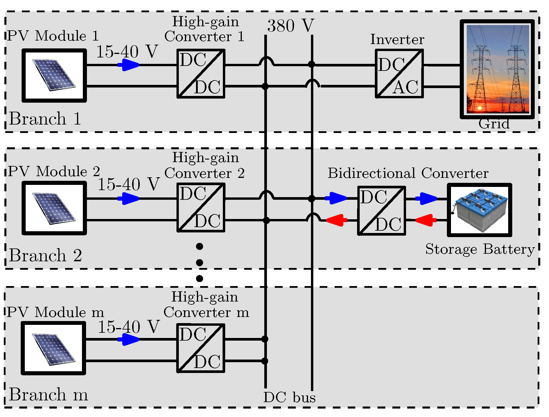
2. System Description and its Mathematical Modeling

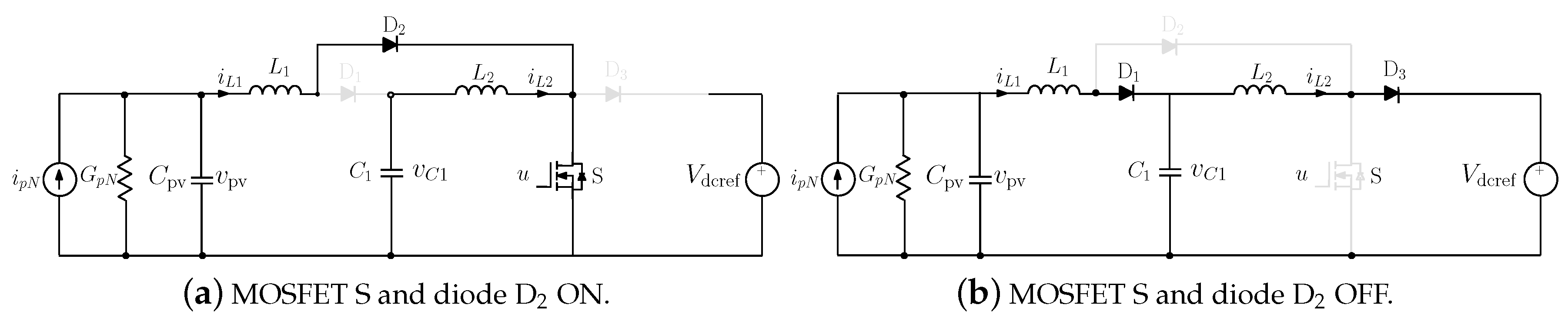
2.1. Operation Principle

The schematic diagram of a DC-DC quadratic boost converter fed by a PV generator and loaded by a DC-AC grid-connected inverter is shown in Figure 2. In this kind of applications, the input voltage is controlled using the switch of the DC-DC stage [27,28,29] while the output DC-link voltage is regulated by acting on the switches of the DC-AC inverter. As the solar irradiation S or the temperature $\mathrm{\Theta }$ change during the operation, the voltage/current of the PV module is adjusted to correspond to the maximum available power. Here, the input port of the DC-DC side is controlled using a resistive control approach for the quadratic boost converter defining the appropriate conductance to match the MPP. This approach is known in the literature as Loss-Free-Resistor (LFR) [26] and it makes the controlled port of the converter to behave like a virtual resistance in average. To achieve this, the reference $i_{\mathrm{ref}}$ for the input current is generated proportionally to the input voltage $v_{\mathrm{pv}}$, i.e, $i_{\mathrm{ref}}=G_{\mathrm{mpp}}{v}_{\mathrm{pv}}$. The proportionality factor $g^{*}=G_{\mathrm{mpp}}$ is a conductance provided by an MPPT controller. The error between the inductor current and the generated reference is controlled by type-II average controller in such a way that the inductor current tightly tracks its reference hence imposing the LFR behavior. The activation of the switch S is carried out as follows: the output $v_{\mathrm{con}}$ of the type-II controller is connected to the inverting pin of the comparator whereas a sawtooth signal $v_{\mathrm{ramp}}=V_M(t/T)\mathrm{mod}1$ is applied to the non inverting pin. The output of the comparator is applied to the reset input of a set-reset (SR) latch and a periodic clock signal is connected to its set input in such a way that the switch S is on at the beginning of each switching cycle and is turned off whenever $v_{\mathrm{con}}=v_{\mathrm{ramp}}$. The state of the diodes D${}_1$ and D${}_3$ are complementary to that of the switch S while that of D${}_2$ is the same as that of S.

Remark 1.

For making the steady-state conductance of the input-stage to match the one corresponding to the MPP, the inductor current has been used instead of the PV current in the synthesis of the LFR. This is because in steady-state, their average values are identical. However, from stability and performance point of view, it is better to use the inductor current which contains both the PV current and the capacitor current. The latter introduces suitable damping and speed-up the system response as detailed in [28].

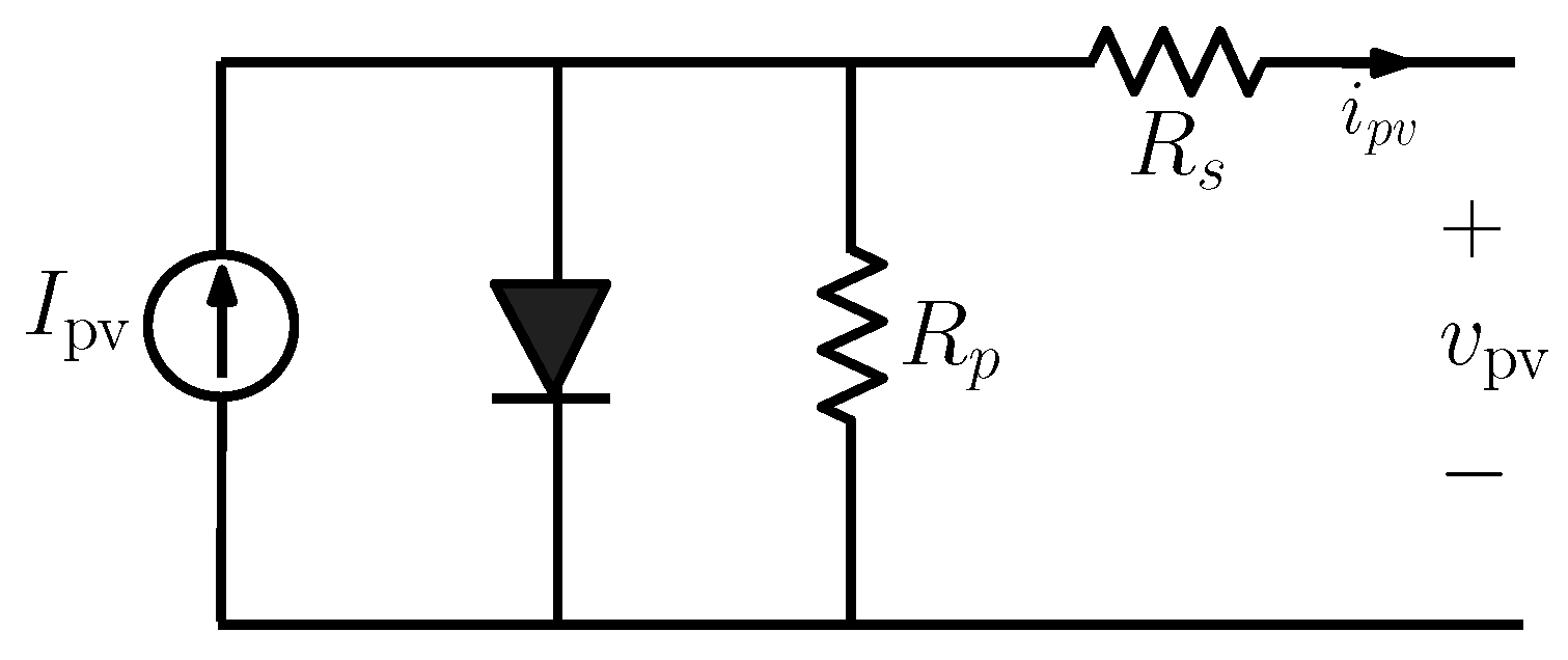
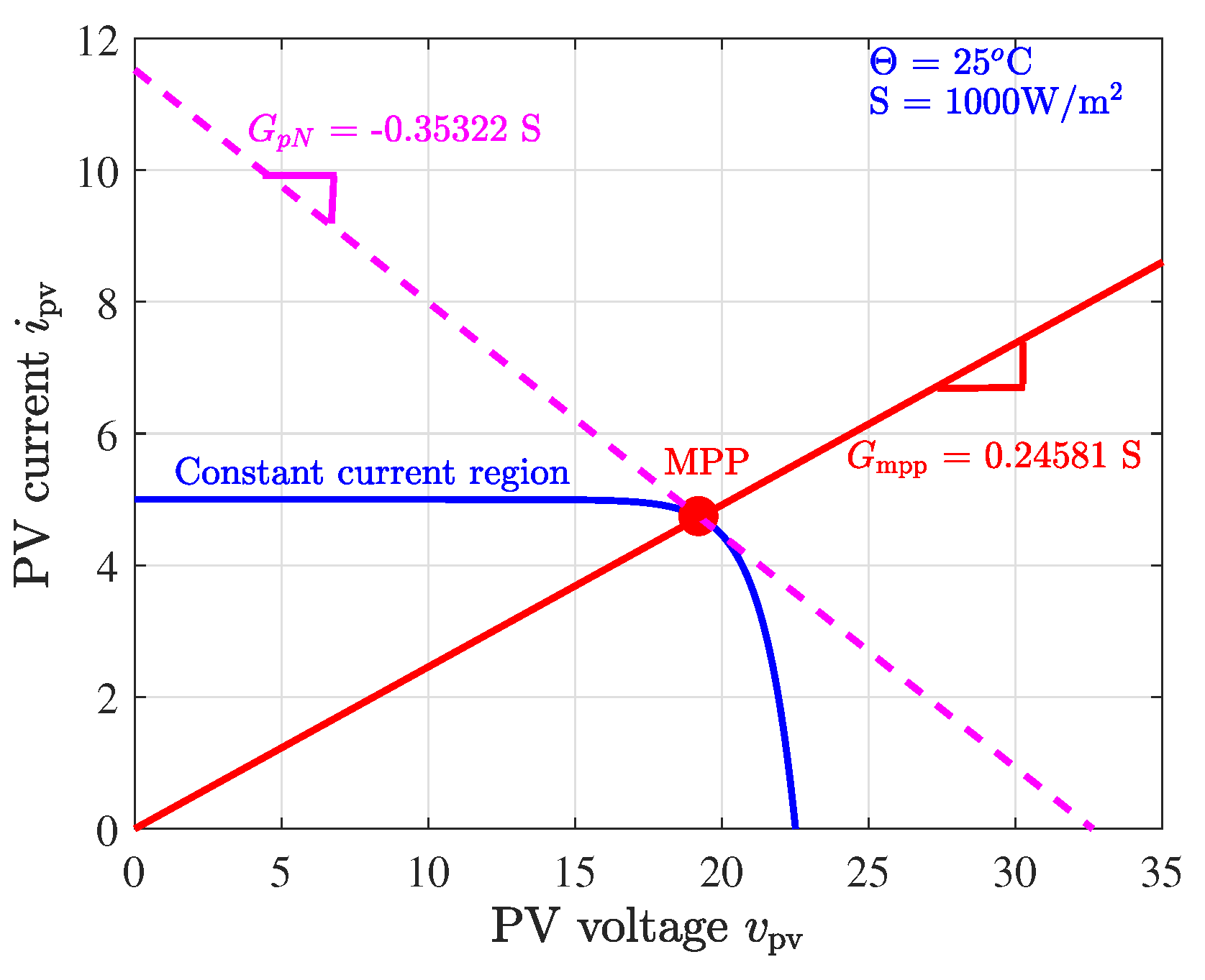
2.2. The Nonlinear Model of a PV Generator

The PV generators have a nonlinear characteristic changing with the temperature $\mathrm{\Theta }$ and irradiation S. Their $i-v$ characteristic equation can be found in many references in the literature. A comparison between the different models are presented in [30]. The single diode model, shown in Figure 3, is one of the most widely used since it has a good compromise between simplicity and accuracy. The equation of this model can be written as follows [31]:

$$i_{\mathrm{pv}}=I_{\mathrm{pv}}-I_s\left(e^{{\displaystyle \frac{v_{\mathrm{pv}}+R_s{i}_{\mathrm{pv}}}{A{V}_t}}}-1\right)-{\displaystyle \frac{v_{\mathrm{pv}}+R_s{i}_{\mathrm{pv}}}{R_p}},$$

(1)

where $i_{\mathrm{pv}}$ and $v_{\mathrm{pv}}$ are, respectively, the current and voltage of the PV module, $I_{\mathrm{pv}}$ and $I_s$ are the photogenerated and saturation currents respectively, $V_t=N_{s}K\theta /q$ is the thermal voltage, A is the diode ideality constant, K is Boltzmann constant, q is the charge of the electron, $\mathrm{\Theta }$ is the PV module temperature and $N_s$ is the number of the series-connected cells. The photogenerated current $I_{\mathrm{pv}}$ depends on the irradiance S and temperature $\mathrm{\Theta }$ according to the following equation:

$$\begin{array}{ccc}\hfill I_{\mathrm{pv}}& =& I_{\mathrm{sc}}{\displaystyle \frac{S}{S_n}}+C_{\mathrm{\Theta }}(\mathrm{\Theta }-{\mathrm{\Theta }}_n),\hfill \end{array}$$

(2)

where $I_{\mathrm{sc}}$ is the short circuit current, ${\mathrm{\Theta }}_n$ and $S_n$ are the nominal temperature and irradiance respectively and $C_{\mathrm{\Theta }}$ is the temperature coefficient. Practical PV generators have a series resistance $R_s$ and a parallel resistance $R_p$. These parameters can be ignored for simplicity.

2.3. The PV Generator Model Close to the MPP

A PV generator has mainly three working regions. Namely, a constant current region where the generator works as a current source, a constant voltage region where the generator works as a voltage source and a maximum power point region where the power drawn from the generator is the optimal one. For a large part of its $i-v$ curve, the PV generator can be considered as a constant current source. However, since the system desired operation is the MPP, this generator can be better linearized by expanding its nonlinear model as a Taylor series and ignoring high-order terms. Therefore, the $i-v$ equation of the PV model can be approximated by the following linear Norton equivalent model:

$$i_{\mathrm{pv}}\approx I_{\mathrm{mpp}}+{\displaystyle \frac{\partial i_{\mathrm{pv}}}{\partial v_{\mathrm{pv}}}}(v_{\mathrm{pv}}-V_{\mathrm{mpp}})=I_{\mathrm{mpp}}+G_{pN}(v_{\mathrm{pv}}-V_{\mathrm{mpp}}).$$

(3)

where $G_{pN}=\partial i_{\mathrm{pv}}/\partial v_{\mathrm{pv}}$ is the equivalent Norton conductance. In contrast to the ideal current source mode, this linearization reveals correctly the effect of the parameters that arise due to the nonlinear nature of the generator such as its dynamic Norton equivalent conductance $G_{pN}$ and its Norton equivalent current $i_{pN}$ that vary with the weather conditions. From (3), and making the PV voltage $v_{\mathrm{pv}}$ zero, the equivalent Norton current $i_{pN}$ is as follows:

$$i_{pN}=I_{\mathrm{mpp}}-G_{pN}{V}_{\mathrm{mpp}},$$

(4)

The equivalent conductance $G_{pN}$ can be obtained by differentiating (1) which by using the implicit function theorem results in the following expression:

$$G_{pN}=-{\displaystyle \frac{A{V}_t+R_p{I}_s{e}^{{\displaystyle \frac{V_{\mathrm{mpp}}+R_s{I}_{\mathrm{mpp}}}{A{V}_t}}}}{A{V}_t(R_p+R_s)+R_p{R}_s{I}_s{e}^{{\displaystyle \frac{V_{\mathrm{mpp}}+R_s{I}_{\mathrm{pv}}}{A{V}_t}}}}}$$

(5)

where $I_{\mathrm{mpp}}$ and $V_{\mathrm{mpp}}$ are the generator current and voltage at the MPP. Based on the data provided in [32], the used PV generator has an open circuit voltage around 22 V under nominal conditions. Its internal parameters are depicted in

Table 1. Parameters of the PV module.

Parameter	Value
Number of cells $N_s$	36
Standard light intensity $S_n$	1000 $\mathrm{W}$/$\mathrm{m}$${}^2$
Ref temperature ${\mathrm{\Theta }}_n$	25 ${}^{\circ }$C
Series resistance $R_s$	0.005 $\mathrm{\Omega }$
Parallel resistance $R_p$	1000 $\mathrm{\Omega }$
Short circuit current $I_{sc}$	$5\mathrm{A}$
Saturation current $I_0$	1.16 $\times {10}^{-8}\mathrm{A}$
Band energy $E_g$	1.12
Ideality factor A	1.2
Temperature coefficient $C_{\mathrm{\Theta }}$	$0.00325\mathrm{A}{/}^{\circ }$C

being its nominal power of $85\mathrm{W}$. It is worth noting that the input voltage of the used PV module varies between 0 and the open circuit voltage with an optimum MPP value of about $18\mathrm{V}$ at nominal weather conditions.

Figure 4 shows its $i-v$ curve together with its linearized approximation close to the MPP for $S=1000$ $\mathrm{W}$/$\mathrm{m}$${}^2$ and $\mathrm{\Theta }=25$ ${}^{\circ }$C. The corresponding load line of the optimum value of the conductance $G_{\mathrm{mpp}}=g^{*}=0.2524$ S is also shown in the same figure.

A PV generator has a single operating point where the power $P=i_{\mathrm{pv}}{v}_{\mathrm{pv}}$ reaches its maximum value $P_{\max }$. The values of the current $I_{\mathrm{mpp}}$ and the voltage $V_{\mathrm{mpp}}$ at this point correspond to a particular load resistance. Its corresponding inductance $G_{\mathrm{mpp}}=g^{*}$ is equal to $I_{\mathrm{mpp}}/V_{\mathrm{mpp}}$. Hence, this generator can operate at the MPP by appropriately selecting that conductance whose load line intersects the $i-v$ curve of the PV generator at the MPP.

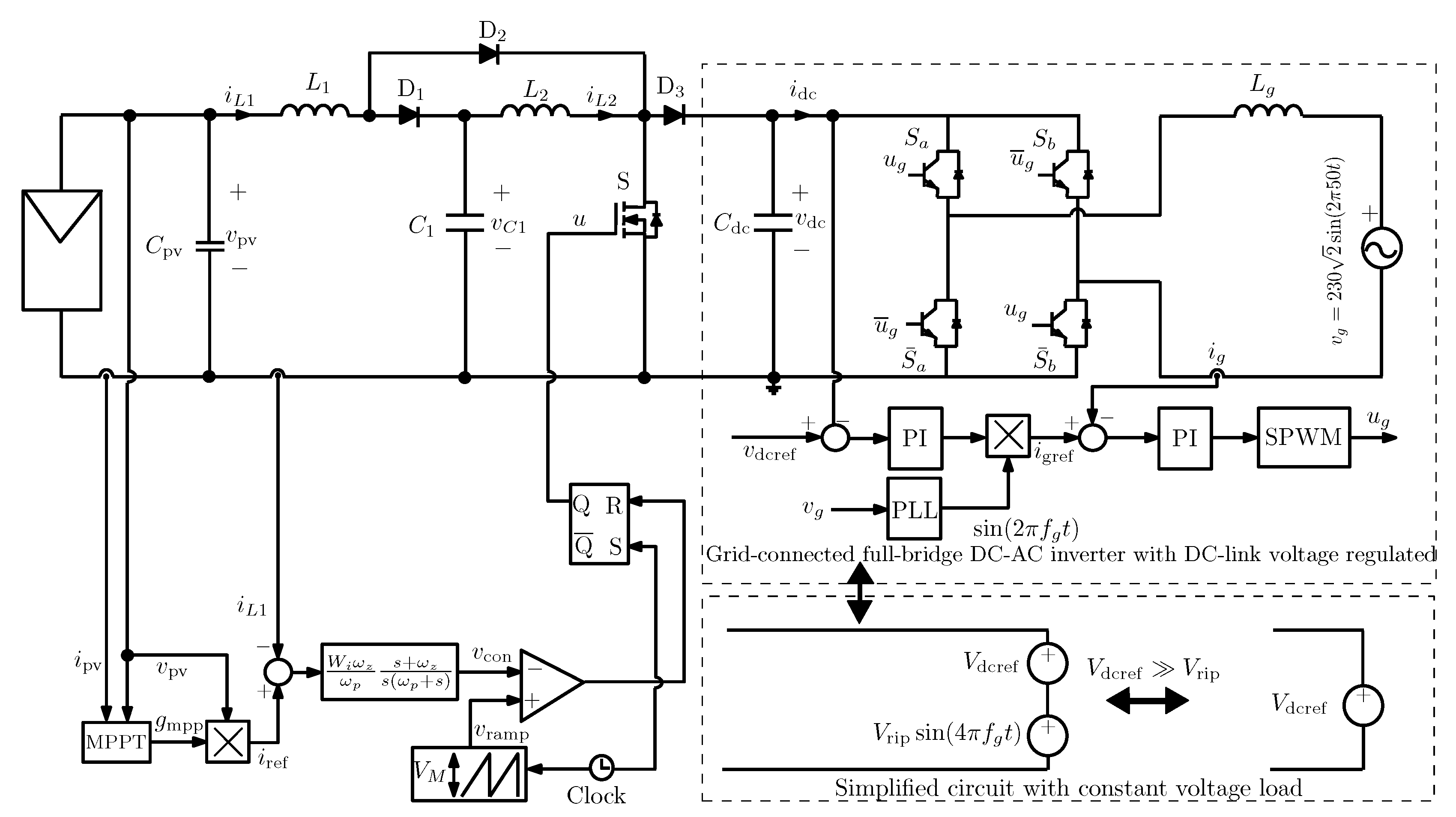
2.4. Modeling of the DC-AC Inverter

The DC-AC inverter stage is responsible for injecting a sinusoidal grid current $i_g$ in phase with the grid voltage $v_g=V_{g}sin\left(2\pi f_{g}t\right)$. For this, a two-loop control strategy is used where the outer DC-link voltage controller provides the reference grid current amplitude $I_{\mathrm{gref}}$ for the inner current controller. This amplitude is multiplied by a sinusoidal signal synchronized with the grid voltage $v_g$, using a phase-locked loop (PLL), to obtain the time varying current reference $i_{\mathrm{g}\mathrm{ref}}=I_{\mathrm{gref}}sin\left(2\pi f_{g}t\right)$. The current controller is conventionally a PI regulator that aims to make the grid current $i_g$ to accurately track $i_{\mathrm{g}\mathrm{ref}}$ hence making the reactive power as close as possible to zero. This outer loop regulates the DC-link voltage by varying the current reference amplitude. A low-pass filter with a cut-off frequency at the grid frequency is also usually added to the PI voltage controller with the aim to reduce the harmonic distortion introduced by second harmonic of the grid frequency. The output of the current controller is fed to a Sinusoidal Pulse Width Modulator (SPWM). The output of this modulator generates the driving signal $u_g$ of the DC-AC H-bridge. The study presented in this paper is constrained to the DC-DC stage assuming a quasi steady-state operation of the DC-AC inverter. This is an accurate assumption provided that the grid voltage $v_g$ and the grid current $i_g$ vary much slower than the variables at the DC-DC stage. The state-space model describing the dynamical behavior of the DC-AC inverter can be written in the following form:

$$\begin{array}{ccc}\hfill {\displaystyle \frac{\mathrm{d}{v}_{\mathrm{dc}}}{\mathrm{d}t}}& =& {\displaystyle \frac{i_{L2}}{C_{\mathrm{dc}}}}(1-u)-{\displaystyle \frac{(2u_g-1)i_g}{C_{\mathrm{dc}}}},\hfill \end{array}$$

(6)

$$\begin{array}{ccc}\hfill {\displaystyle \frac{\mathrm{d}{i}_g}{\mathrm{d}t}}& =& (2u_g-1){\displaystyle \frac{v_{\mathrm{dc}}}{L_g}}-{\displaystyle \frac{v_g}{L_g}}.\hfill \end{array}$$

(7)

A simple steady-state analysis based on a power balance reveals that the DC-link voltage can be approximated by:

$$v_{\mathrm{dc}}\approx V_{\mathrm{dcref}}+V_{\mathrm{rip}}sin\left(4\pi f_{g}t\right),$$

(8)

where $V_{\mathrm{rip}}$ is the amplitude of the ripple at the double frequency of the grid which can be expressed as follows [33]:

$$V_{\mathrm{rip}}={\displaystyle \frac{\eta P_{\mathrm{pv}}}{4\pi f_g{C}_{\mathrm{dc}}{V}_{\mathrm{dcref}}}},$$

(9)

$\eta$ is the efficiency of the DC stage, $f_g$ is the grid frequency, $C_{\mathrm{dc}}$ is the DC-link capacitance and $V_{\mathrm{dcref}}$ is the desired DC-link voltage. For a well designed inverter, one has $V_{\mathrm{dcref}}\gg V_{\mathrm{rip}}$. Moreover, the switching frequency is much higher than the grid frequency and therefore, the DC-link voltage can be considered constant at the switching time-scale. This is a widely used assumption in two-stage PV systems when the design of the DC-DC stage is of concern [24,25,28].

2.5. Dynamic Modeling of the Quadratic Boost Regulator Powered by a PV Generator

In PV systems, the input voltage of the DC-DC converter is controlled, not its output voltage. Therefore, it is modeled and analyzed as a current-fed converter. If the Norton equivalent model of the PV generator is used and the DC-link voltage ripple is neglected, the circuit configurations of the quadratic boost converter corresponding to the two different switch states are the ones depicted in Figure 5a,b.

The application of Kirchhoff’s laws to the circuit, after substituting the nonlinear PV generator by its Norton equivalent model, leads to the following set of differential equations describing the quadratic boost converter dynamical behavior:

$$\begin{array}{ccc}\hfill {\displaystyle \frac{\mathrm{d}{v}_{\mathrm{pv}}}{\mathrm{d}t}}& =& {\displaystyle \frac{i_{pN}}{C_{\mathrm{pv}}}}-{\displaystyle \frac{G_{pN}{v}_{\mathrm{pv}}}{C_{\mathrm{pv}}}}-{\displaystyle \frac{i_{L1}}{C_{\mathrm{pv}}}},\hfill \end{array}$$

(10)

$$\begin{array}{ccc}\hfill {\displaystyle \frac{\mathrm{d}{i}_{L1}}{\mathrm{d}t}}& =& {\displaystyle \frac{v_{\mathrm{pv}}}{L_1}}-{\displaystyle \frac{v_{C1}}{L_1}}(1-u),\hfill \end{array}$$

(11)

$$\begin{array}{ccc}\hfill {\displaystyle \frac{\mathrm{d}{i}_{L2}}{\mathrm{d}t}}& =& {\displaystyle \frac{v_{C1}}{L_2}}-{\displaystyle \frac{V_{\mathrm{dcref}}}{L_2}}(1-u),\hfill \end{array}$$

(12)

$$\begin{array}{ccc}\hfill {\displaystyle \frac{\mathrm{d}{v}_{C1}}{\mathrm{d}t}}& =& {\displaystyle \frac{i_{L1}}{C_1}}(1-u)-{\displaystyle \frac{i_{L2}}{C_1}},\hfill \end{array}$$

(13)

where $L_1$ and $L_2$ are the inductances of the input and intermediate inductors, $C_{\mathrm{pv}}$ and $C_1$ are the capacitances of the input and the intermediate capacitors. All other parameters and variables that appear in (10)–(13) are shown in Figure 2. By applying a net volt-second balance [3], the following expressions are obtained relating the average steady-state values of the state variables to the operating duty cycle D:

$$\begin{array}{c}{I}_{L1}=i_{pN}-G_{pN}{V}_{\mathrm{mpp}},I_{L2}=(1-D)I_{L1},\end{array}$$

(14)

$$\begin{array}{c}{V}_{C1}=V_{\mathrm{dcref}}(1-D),V_{\mathrm{pv}}=V_{\mathrm{mpp}}=V_{\mathrm{dcref}}{(1-D)}^2.\hfill \end{array}$$

(15)

From (15), it can be observed that for a fixed value of D, the main advantage of the quadratic boost converter is that the voltage conversion gain defined as $V_{\mathrm{dcref}}/V_{\mathrm{pv}}$ is the square of the conversion ratio corresponding to the canonical boost converter. According to (15), D is related to the PV generator average voltage $V_{\mathrm{pv}}=V_{\mathrm{mpp}}$ and the average output voltage $V_{\mathrm{dcref}}$ by the following expression:

$$D(S,\mathrm{\Theta })=1-\sqrt{{\displaystyle \frac{V_{\mathrm{mpp}}(S,\mathrm{\Theta })}{V_{\mathrm{dcref}}}}}.$$

(16)

For a slowly-varying output voltage, the quasi-steady-state duty cycle D is a function of the climatic conditions, and it is constrained by (16) with $V_{\mathrm{mpp}}$ as a function of the temperature $\mathrm{\Theta }$ and the irradiance S.

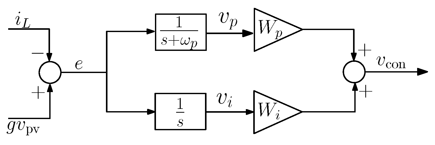
2.6. Modeling the Input Port Controller

Since a dynamic controller is used for controlling the input port of the quadratic boost converter, its corresponding state equations are needed to complete the system model. The transfer function of the type-II controller is as follows:

$$\begin{array}{ccc}\hfill H_i\left(s\right)& =& {\displaystyle \frac{W_i{\omega }_p}{{\omega }_z}}{\displaystyle \frac{s+{\omega }_z}{s(s+{\omega }_p)}},\hfill \end{array}$$

(17)

where $W_i$ is the integrator gain, ${\omega }_z$ is the cut-off frequency of the controller zero and ${\omega }_p$ is the cut-off frequency of its pole. Let $W_p=({\omega }_p-{\omega }_z)W_i/{\omega }_z$. A partial fraction decomposition of the transfer function defined in (17) lead to the following equivalent form which is suitable to be converted to a state space representation [34]:

$$\begin{array}{ccc}\hfill H_i\left(s\right)& =& {\displaystyle \frac{W_i}{s}}+{\displaystyle \frac{W_p}{s+{\omega }_p}},\hfill \end{array}$$

(18)

Figure 6 shows an equivalent block diagram of the type-II controller where its corresponding state variables are represented together with their weighting factors in the feedback loop. From this block diagram, the time-domain state equations corresponding to the previous Laplace domain transfer function can be expressed as follows:

$$\begin{array}{ccc}\hfill {\displaystyle \frac{\mathrm{d}{v}_p}{\mathrm{d}t}}& =& -{\omega }_p{v}_p+G_{\mathrm{mpp}}{v}_{\mathrm{pv}}-i_{L1},\hfill \end{array}$$

(19)

$$\begin{array}{ccc}\hfill {\displaystyle \frac{\mathrm{d}{v}_i}{\mathrm{d}t}}& =& G_{\mathrm{mpp}}{v}_{\mathrm{pv}}-i_{L1}.\hfill \end{array}$$

(20)

where $v_p$ and $v_i:=\int (G_{\mathrm{mpp}}{v}_{\mathrm{pv}}-i_{L1})\mathrm{d}t$ are the state variables corresponding to the type-II controller [35].

2.7. The State-Space Switched Model of the Quadratic Boost Converter

The model of the quadratic boost converter given in (10)–(13) can be written in the following matrix form:

$$\begin{array}{ccc}\hfill {\dot{\mathbf{x}}}_p& =& {\mathbf{A}}_{p1}{\mathbf{x}}_p+{\mathbf{B}}_{p1}{\mathbf{w}}_p\mathrm{if}u=1\hfill \end{array}$$

(21)

$$\begin{array}{ccc}\hfill {\dot{\mathbf{x}}}_p& =& {\mathbf{A}}_{p0}{\mathbf{x}}_p+{\mathbf{B}}_{p0}{\mathbf{w}}_p\mathrm{if}u=0\hfill \end{array}$$

(22)

$$\begin{array}{ccc}\hfill e& =& G_{\mathrm{mpp}}{v}_{\mathrm{pv}}-i_{L1}:={\mathbf{C}}_p^{⊺}{\mathbf{x}}_p\hfill \end{array}$$

(23)

where ${\mathbf{x}}_p={(v_{\mathrm{pv}},i_{L1},i_{L2},v_{C1})}^{⊺}$ is the vector of the state variables of the converter and ${\mathbf{A}}_{pu}$ and ${\mathbf{B}}_{pu}$, $u=1,0$, are the state and input matrices corresponding to the different switch states. According to (10)–(13), the matrices ${\mathbf{A}}_{pu}$ and ${\mathbf{B}}_{pu}$ for $u=1$ and $u=0$, and the external input parameters vector ${\mathbf{w}}_p$ are as follows:

$$\begin{array}{ccc}\hfill {\mathbf{A}}_{p1}& =& \left(\begin{array}{cccc}-{\displaystyle \frac{G_{pN}}{C_{pN}}}& -{\displaystyle \frac{1}{C_{\mathrm{pv}}}}& 0& 0\\ {\displaystyle \frac{1}{L_1}}& 0& 0& 0\\ 0& 0& 0& {\displaystyle \frac{1}{L_2}}\\ 0& 0& -{\displaystyle \frac{1}{C_1}}& 0\end{array}\right),{\mathbf{A}}_{p0}=\left(\begin{array}{cccc}-{\displaystyle \frac{G_{pN}}{C_{pN}}}& -{\displaystyle \frac{1}{C_{\mathrm{pv}}}}& 0& 0\\ {\displaystyle \frac{1}{L_1}}& 0& 0& 0\\ 0& 0& 0& {\displaystyle \frac{1}{L_2}}\\ 0& {\displaystyle \frac{1}{C_1}}& -{\displaystyle \frac{1}{C_1}}& 0\end{array}\right),\hfill \end{array}$$

(24)

$$\begin{array}{ccc}\hfill {\mathbf{B}}_{p1}& =& \left(\begin{array}{cc}{\displaystyle \frac{1}{C_{\mathrm{pv}}}}& 0\\ 0& 0\\ 0& -{\displaystyle \frac{1}{L_2}}\\ 0& 0\end{array}\right),{\mathbf{B}}_{p0}=\left(\begin{array}{cc}{\displaystyle \frac{1}{C_{\mathrm{pv}}}}& 0\\ 0& 0\\ 0& 0\\ 0& 0\end{array}\right),{\mathbf{w}}_p=\left(\begin{array}{c}{i}_{pN}\\ V_{\mathrm{dcref}}\end{array}\right).\hfill \end{array}$$

(25)

3. Small-Signal Model of the DC-DC Quadratic Boost Converter and Its Input Controller Design

The design of the controller in a switching converter is conventionally based on a small-signal averaged model, which can be obtained from (10)–(13) after substituting the control signal u by its duty cycle d and performing a perturbation and linearization close to the operating point of the converter.

The averaged small-signal model of the quadratic boost power stage can be expressed in the state-space form ${\dot{\tilde{\mathbf{x}}}}_p=\mathbf{A}\tilde{\mathbf{x}}+\mathbf{B}$$\tilde{d}$, where $\tilde{}$ stands for a small-signal variation, $\mathbf{A}={\mathbf{A}}_{p1}D+{\mathbf{A}}_{p0}(1-D)$ and $\mathbf{B}=({\mathbf{A}}_{p1}-{\mathbf{A}}_{p0}){\mathbf{x}}_{\mathrm{av}}+{\mathbf{B}}_{p1}-{\mathbf{B}}_{p0}$ and ${\mathbf{x}}_{\mathrm{av}}=-{\mathbf{A}}^{-1}({\mathbf{B}}_{p1}D+{\mathbf{B}}_{p0}(1-D)$. Selecting the output represented by the small-signal error signal $\tilde{e}={\tilde{i}}_{L1}-G_{\mathrm{mpp}}{\tilde{v}}_{\mathrm{pv}}$ and using the Laplace transform, the small-signal transfer functions can be straightforwardly obtained using the well-known formula $\tilde{e}\left(s\right)={\mathbf{C}}_p^{⊺}{(s\mathbf{I}-\mathbf{A})}^{-1}\mathbf{B}\tilde{d}$, where ${\mathbf{C}}_p^{⊺}=(G_{\mathrm{mpp}}-100)$ and $\mathbf{I}$ is a 4 × 4 identity matrix. Hence, the d-to-e transfer function can be expressed as follows:

$$H_p\left(s\right)={\mathbf{C}}_p^{⊺}{(s\mathbf{I}-\mathbf{A})}^{-1}\mathbf{B}$$

(26)

The zeros can be obtained by solving for s the equation ${\mathbf{C}}_p^{⊺}{(s\mathbf{I}-\mathbf{A})}^{-1}\mathbf{B}=0$. In doing so and after some algebra taking into account (14)–(15), the following expressions for the zeros are obtained:

$$\begin{array}{ccc}\hfill z_1& =& -{\displaystyle \frac{G_{pN}+G_{\mathrm{mpp}}}{C_p}},\hfill \end{array}$$

(27)

$$\begin{array}{ccc}\hfill z_2& =& {\displaystyle \frac{-I_{\mathrm{mpp}}}{2C_1{V}_{\mathrm{dcref}}}}+j{\displaystyle \frac{\sqrt{8C_1/L_2{V}_{\mathrm{dcref}}^2-I_{L1}^2}}{2C_1{V}_{\mathrm{dcref}}}}\hfill \end{array}$$

(28)

$$\begin{array}{ccc}\hfill z_3& =& {\displaystyle \frac{-I_{\mathrm{mpp}}}{2C_1{V}_{\mathrm{dcref}}}}-j{\displaystyle \frac{\sqrt{8C_1/L_2{V}_{\mathrm{dcref}}^2-I_{L1}^2}}{2C_1{V}_{\mathrm{dcref}}}}\hfill \end{array}$$

(29)

Note that in addition to the left half plane zero $z_1$, which also exists in the small-signal model of the canonical boost converter with input current feedback, an extra complex conjugate zeros pair appears in the small-signal model of the quadratic boost converter. Note also that because $8C_1/L_2{V}_{\mathrm{dcref}}^2-I_{L1}^2>0$, the extra complex conjugate zeros are located in the left half side of the complex plane, and therefore, the input controlled quadratic boost converter is a minimum phase system. This is also the case of the boost converter with input voltage feedback [36]. On the other hand, the poles can be obtained by solving for s the equation $det(s\mathbf{I}-{\mathbf{A}}_{\mathrm{ss}})=0$, i.e.,

$$s^4+a_3{s}^3+a_2{s}^2+a_{1}s+a_0=0$$

(30)

where the coefficients $a_3$, $a_2$, $a_1$, and $a_0$ are given by the following expressions:

$$a_3={\displaystyle \frac{G_{\mathrm{pN}}}{C_p}},a_2={\displaystyle \frac{C_p{L}_1+L_2(C_1+C_p{(1-D)}^2)}{C_1{C}_p{L}_1{L}_2}},a_1={\displaystyle \frac{G_{\mathrm{pN}}(L_1+L_2{(1-D)}^2)}{C_1{C}_p{L}_1{L}_2}},a_0={\displaystyle \frac{1}{C_1{C}_p{L}_1{L}_2}}.$$

(31)

It is worth noting that the desired working point of the PV source is the MPP characterized by a Norton equivalent conductance $G_{pN}\ne 0$. In this case, according to Routh-Hurwitz criterion, all the poles of the quadratic boost converter are located in the left half side of the complex plane. However, if under any circumstance, such as at startup or during a transient, the PV source works in the constant current region characterized by a zero Norton equivalent conductance, the quadratic boost converter will exhibit two pairs of purely imaginary complex conjugate poles that can lead to undamped low frequency oscillation. With an appropriate control design, such oscillation will disappear as soon as the system reaches the operation in the MPP mode forced by the MPPT controller.

Using the previously-obtained small-signal model, the input port controller design can be performed by appropriately selecting the required performances in terms of settling time, crossover frequency, and stability phase margin. With this averaged small-signal approach, the controller is designed for the lowest irradiance level [14]. Figure 7 shows the crossover frequency $f_c$ and the phase margin ${\phi }_m$ of the model of the quadratic boost converter under the type-II input port controller when the irradiance is varied in the range (500, 1000) $\mathrm{W}/{\mathrm{m}}^2$. According to the small-signal averaged model, as the irradiance level is increased, the crossover frequency $f_c$ increases at the expense of a decrease of the phase margin ${\phi }_m$. Despite this, according to the same model, the system remains stable and exhibits a sufficient phase margin above 40${}^{\circ }$ and an infinite gain margin for the whole range of the varied parameter. The gain margin is infinite because the total loop gain presents six stable poles (four from the power stage and two from the controller) and four stable zeros (three from the power stage and one from the controller), and the asymptotic behavior at high frequencies is similar to a minimum phase continuous-time second order system whose phase never crosses −180 degrees; therefore, the gain can be increased as much as possible without destabilizing the system. However, the values of the gain and the phase obtained from the small-signal average model are different from the actual phase of the switched system in the vicinity of the Nyquist frequency, as was recently reported in [37]. Indeed, it will be shown later using accurate discrete-time modeling that the system exhibits instability in the form of subharmonic oscillation for values of irradiance larger than approximately 820 $\mathrm{W}/{\mathrm{m}}^2$ with the fixed values of parameters shown in Table 1,

Table 2. The parameters used for the DC-AC inverter.

Parameter	Value
Inductance $L_g$	20 mH
DC-link capacitance $C_{\mathrm{DC}}$	47 $\mathsf{\mu }$F
Grid frequency $f_g$	50 Hz
PWM switching frequency $f_s$	50 kHz
RMS value of the grid voltage	230 V
Proportional gain (current) $k_{ip}$	1 $\mathrm{\Omega }$
Integral gain (current) $k_{ii}$	20 krad/s
Cut-off frequency of the filter (current controller)	50 Hz
Proportional gain (voltage) $k_{vp}$	0.019
Integral gain (voltage) $k_{vi}$	0.51 rad/s

and

Table 3. The parameter values used for the quadratic boost converter.

${\mathit{L}}_1$ ($\mathsf{\mu }$H)	${\mathit{L}}_2$ (mH)	${\mathbf{C}}_1$, ${\mathbf{C}}_{\mathit{pv}}$, ${\mathbf{C}}_{\mathit{dc}}$($\mathsf{\mu }\mathit{F}$)	${\mathit{V}}_{\mathit{M}}$ (V)	${\mathit{V}}_{\mathit{g}}$ (V)	${\mathit{V}}_{\mathit{dcref}}$ (V)	${\mathit{\omega }}_{\mathit{p}}$, ${\mathit{\omega }}_{\mathit{z}}$, ${\mathit{W}}_{\mathit{i}}$ (krad/s)	${\mathit{f}}_{\mathit{s}}$ (kHz)
120–138	3.5–5.5	10, 10, 47	variable	230$\sqrt{2}$	380	50$\pi$, 1, 1	50

.

4. The Complete State-Space Switched Model of the Closed-Loop Quadratic Boost Regulator

The complete model of the quadratic boost regulator is obtained by including the state variables corresponding to the input port controller. This model can be written in the following augmented matrix form:

$$\begin{array}{ccc}\hfill \dot{\mathbf{x}}& =& {\mathbf{A}}_1\mathbf{x}+{\mathbf{B}}_1\mathbf{w}\mathrm{if}u=1,\hfill \end{array}$$

(32)

$$\begin{array}{ccc}\hfill \dot{\mathbf{x}}& =& {\mathbf{A}}_0\mathbf{x}+{\mathbf{B}}_0\mathbf{w}\mathrm{if}u=0,\hfill \end{array}$$

(33)

$$\begin{array}{ccc}\hfill {\dot{v}}_i& =& e=G_{\mathrm{mpp}}{v}_{\mathrm{pv}}-i_{L1}.\hfill \end{array}$$

(34)

where $\mathbf{x}={(v_{\mathrm{pv}},i_{L1},i_{L2},v_{C1},v_p)}^{⊺}$ is the augmented vector of state variables, ${\mathbf{A}}_0\in {\mathbb{R}}^{5\times 5}$, ${\mathbf{A}}_1\in {\mathbb{R}}^{5\times 5}$, ${\mathbf{B}}_0\in {\mathbb{R}}^{5\times 2}$ and ${\mathbf{B}}_1\in {\mathbb{R}}^{5\times 2}$ are the augmented system state matrices taking into account the state variables of the power stage and the controller and excluding the state variable corresponding to the integral action and $\mathbf{w}={(i_{pN},V_{\mathrm{dcref}})}^{⊺}$ is the vector of the external parameters supposed to be constant within a switching cycle. To avoid matrix singularity problems in computer computations and to start with a well-posed mathematical problem, the state variable $v_i$ was excluded from the rest of state variables in the vector $\mathbf{x}$ [35]. According to (10)–(13) and (19), the matrices ${\mathbf{A}}_u$ and ${\mathbf{B}}_u$ and the input vector $\mathbf{w}$ for $u=1$ and $u=0$ are as follows:

$$\begin{array}{c}\hfill {\mathbf{A}}_1=\left(\begin{array}{ccccc}-{\displaystyle \frac{G_{pN}}{C_{pN}}}& -{\displaystyle \frac{1}{C_{\mathrm{pv}}}}& 0& 0& 0\\ {\displaystyle \frac{1}{L_1}}& 0& 0& 0& 0\\ 0& 0& 0& {\displaystyle \frac{1}{L_2}}& 0\\ 0& 0& -{\displaystyle \frac{1}{C_1}}& 0& 0\\ G_{\mathrm{mpp}}& -1& 0& 0& -{\omega }_p\end{array}\right),{\mathbf{A}}_0=\left(\begin{array}{ccccc}-{\displaystyle \frac{G_{pN}}{C_{pN}}}& -{\displaystyle \frac{1}{C_{\mathrm{pv}}}}& 0& 0& 0\\ {\displaystyle \frac{1}{L_1}}& 0& 0& 0& 0\\ 0& 0& 0& {\displaystyle \frac{1}{L_2}}& -{\displaystyle \frac{1}{L_1}}\\ 0& {\displaystyle \frac{1}{C_1}}& -{\displaystyle \frac{1}{C_1}}& 0& 0\\ G_{\mathrm{mpp}}& -1& 0& 0& -{\omega }_p\end{array}\right),\end{array}$$

(35)

$$\begin{array}{ccc}\hfill {\mathbf{B}}_1& =& \left(\begin{array}{cc}{\displaystyle \frac{1}{C_{\mathrm{pv}}}}& 0\\ 0& 0\\ 0& -{\displaystyle \frac{1}{L_2}},\\ 0& 0\\ 0& 0\end{array}\right),{\mathbf{B}}_0=\left(\begin{array}{cc}{\displaystyle \frac{1}{C_{\mathrm{pv}}}}& 0\\ 0& 0\\ 0& 0\\ 0& 0\\ 0& 0\end{array}\right),\mathbf{w}=\left(\begin{array}{c}{i}_{pN}\\ V_{\mathrm{dcref}}\end{array}\right).\hfill \end{array}$$

(36)

5. A Glimpse at the Solar PV System Behavior from Its Complete Mathematical Model

Let us take a quick glimpse at some of the typical operating dynamic behaviors of the system in terms of different parameter values. The numerical simulations are performed using PSIM^© software using the detailed switched model of the complete system consisting of the DC-DC quadratic boost converter performing MPPT and interlinked to the grid-connected DC-AC inverter as depicted in Figure 2. The nonlinear PV panel model is implemented using the physical model of the solar module in the renewable energy package of PSIM^©. The set of parameter values shown in Table 3 is used for the quadratic boost converter, those in Table 1 for the PV module, and the ones in Table 2 for the DC-AC inverter. The inductance values were selected to guarantee continuous conduction mode (CCM), and the capacitance values were chosen to get acceptable voltage ripple amplitudes. The compensator zero ${\omega }_z=$ 1 krad/s was placed in such a way to damp partially one of the complex conjugate poles pair resonant effect. The low-pass filter pole ${\omega }_p$ was placed at one half the switching frequency. An extremum seeking algorithm was used for performing MPPT [38,39].

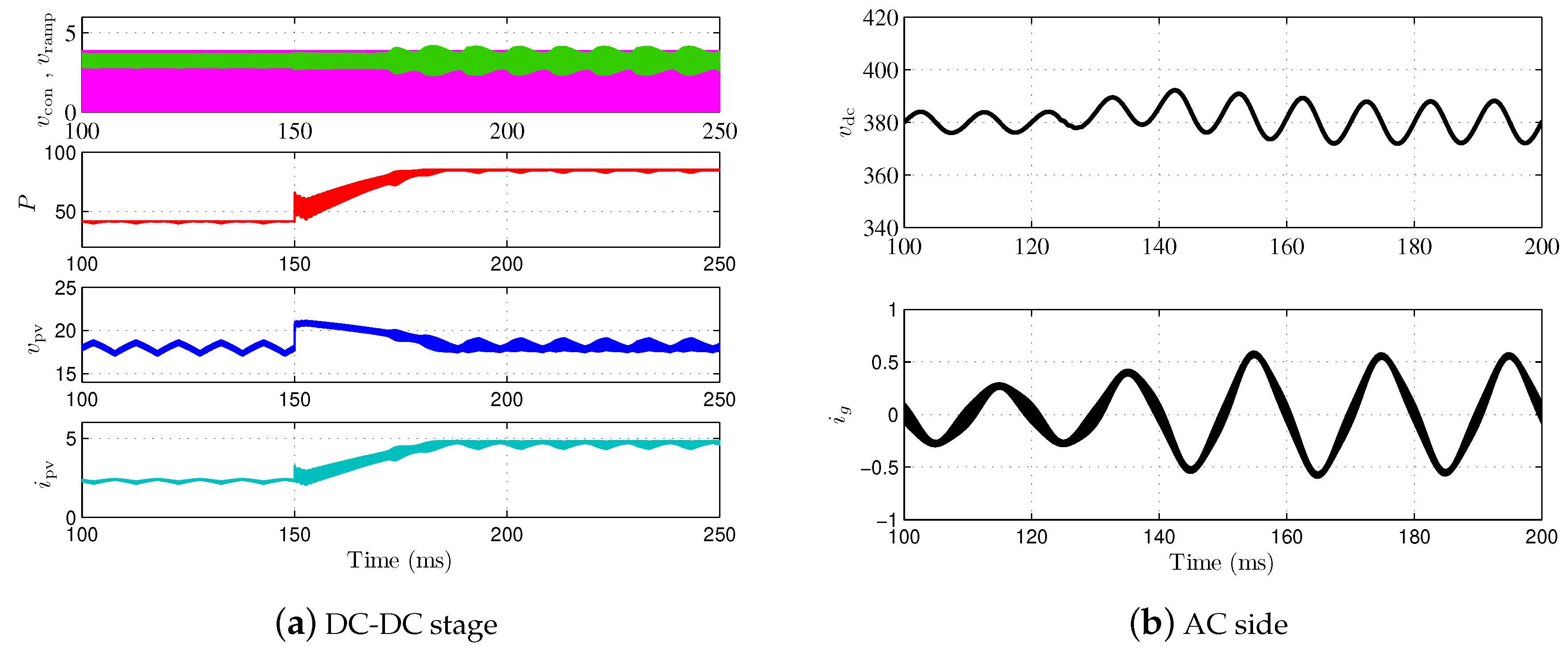
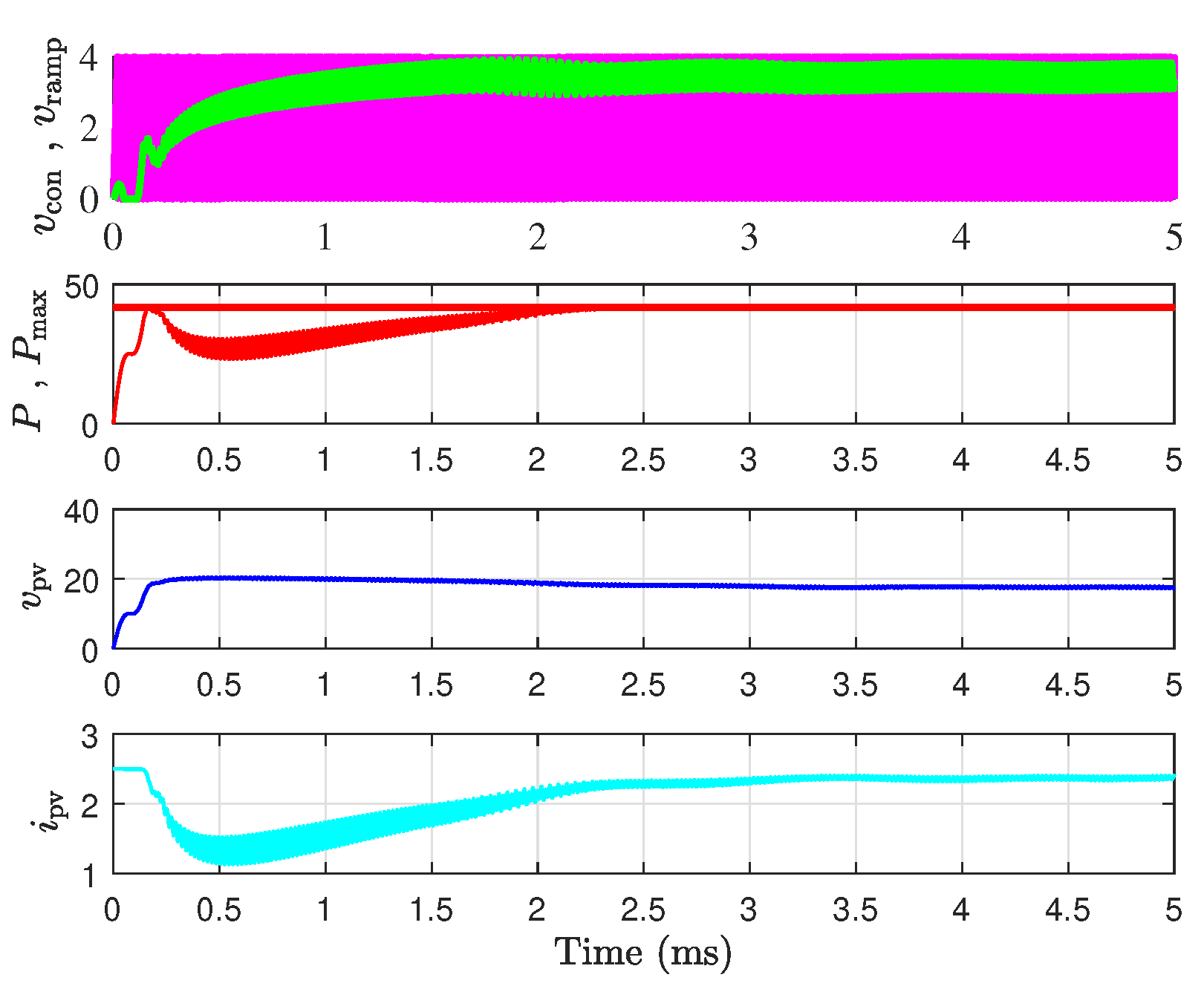
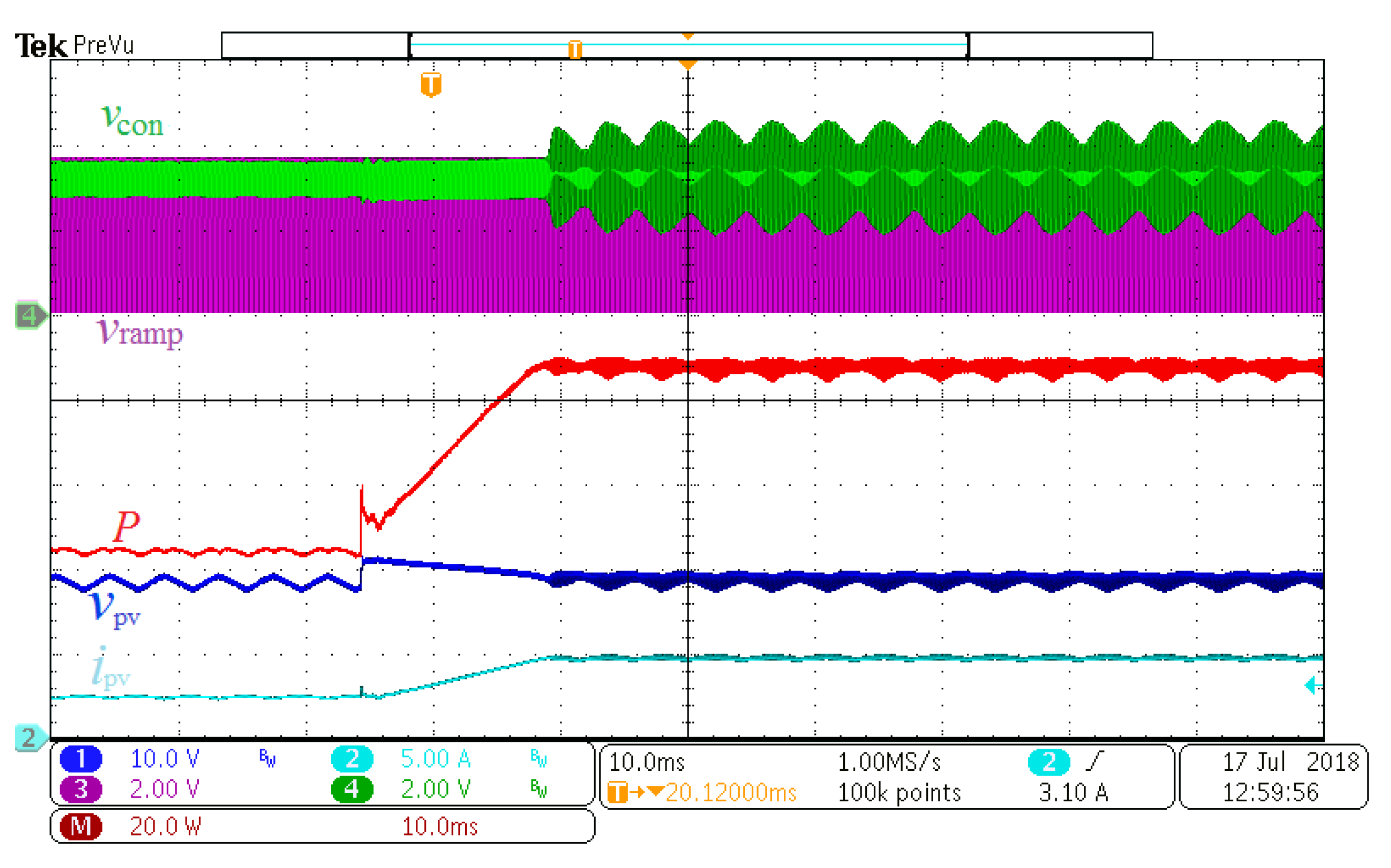
5.1. System Startup and Steady-State Response

The response of the complete system starting from zero initial conditions is depicted in Figure 8. It can be seen from the plots that after an initial transient, the state variables and the control signals of the system reached their desired periodic steady-state. The extracted power also converged to its MPP value.

Figure 9a illustrates the response of the system to a change in the irradiance level from 500 $\mathrm{W}/{\mathrm{m}}^2$ ($P_{\max }\approx 42$ W) to 1000 $\mathrm{W}/{\mathrm{m}}^2$ ($P_{\max }\approx 85$ W). In that figure, the waveforms of the control signals $v_{\mathrm{ramp}}$ and $v_{\mathrm{con}}$, the instantaneous power P, its reference value $P_{\max }$ are depicted. The DC link voltage and the grid current in the AC side are also shown in the same figure. A detailed view of the ramp modulator, the control signal and the inductor currents at DC-DC stage is shown in Figure 10 where it can be observed that desired periodic operation (stable) takes place for $S=500$ $\mathrm{W}/{\mathrm{m}}^2$ while nonlinear phenomena in the form of subharmonic oscillation is exhibited for $S=1000$ $\mathrm{W}/{\mathrm{m}}^2$. It is worth noting that the dynamical behavior and the stability at the AC side is not affected by the subharmonic oscillation at the DC side as can be observed in Figure 9b. Moreover, the grid current $i_g$ exhibits a low total harmonic distortion of about $2\%$ as calculated by PSIM^© software.

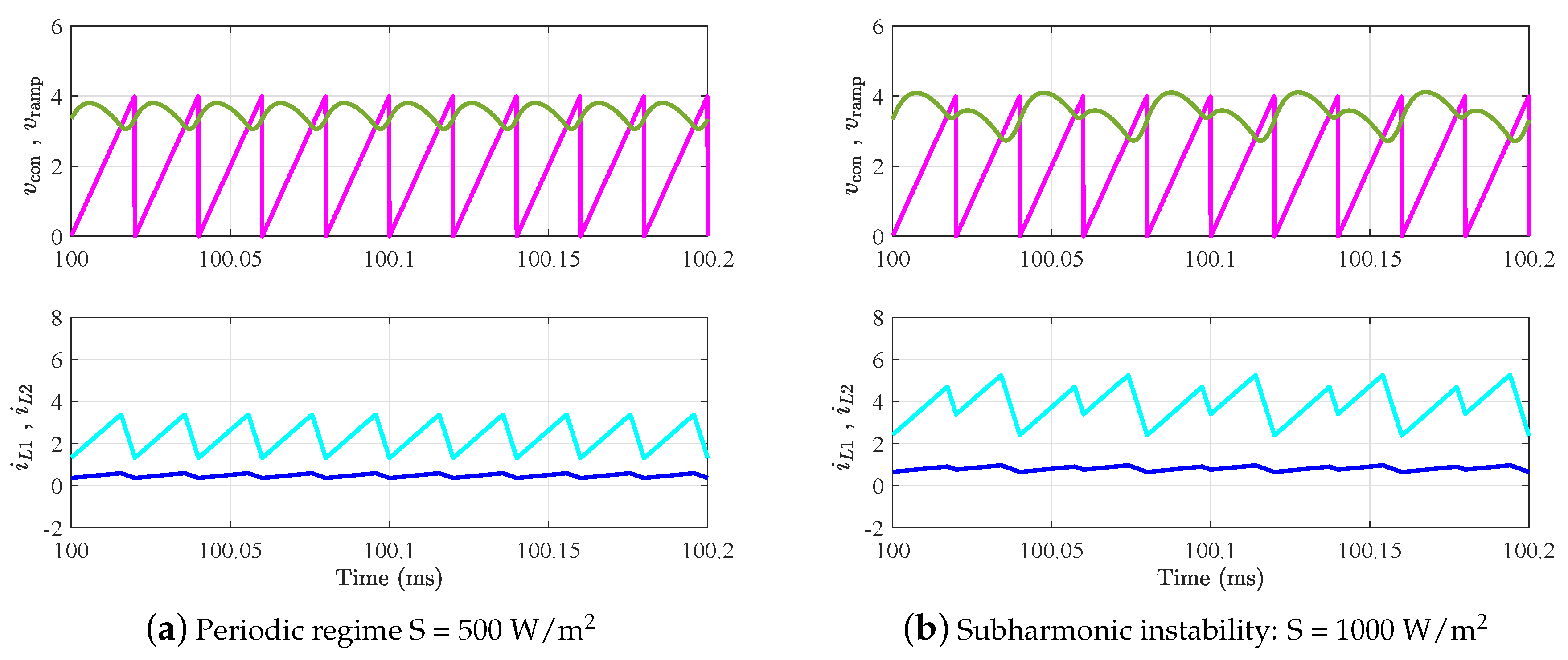
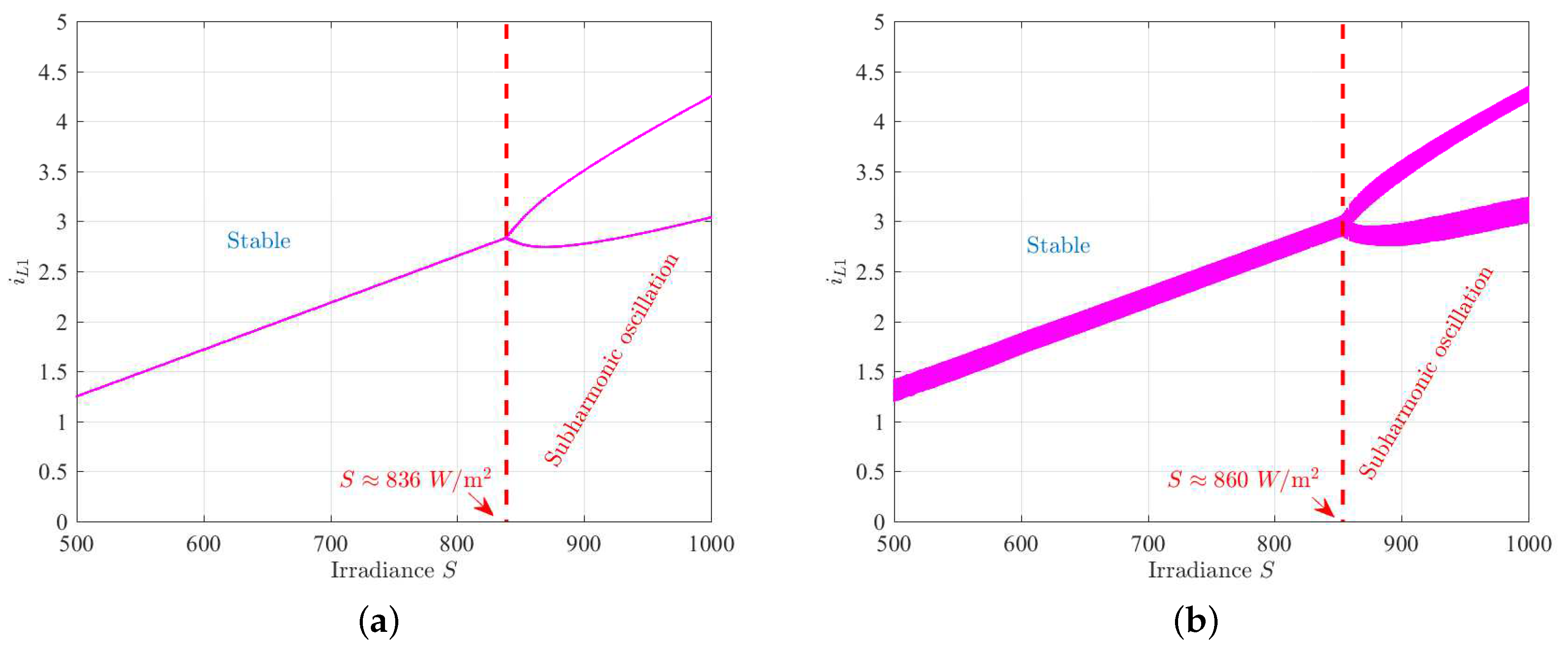
5.2. Bifurcation Diagram of the PV System by Varying the Irradiance Level

In order to understand the mechanisms of how the subharmonic oscillation takes place, a bifurcation diagram for the system is plotted by considering the irradiance S as a bifurcation parameter which is varied within the range (500, 1000) $\mathrm{W}/{\mathrm{m}}^2$. This bifurcation diagram is obtained by sampling the vector of state variables $\mathbf{x}\left(t\right)$ at the switching period rate, thus yielding $\mathbf{x}\left(nT\right)$, $n=0,1\dots 100\times {10}^3$. The last 100 samples are considered as steady-state and the corresponding inductor current samples $i_{L1}\left(nT\right)$ are plotted in terms of the bifurcation parameter. Two bifurcation diagrams were computed and the results are shown in Figure 11. In the first diagram, a constant value $g^{*}$ of the conductance was used for simplicity. In the second one, the dynamic conductance $G_{\mathrm{mpp}}$ provided by the extremum seeking MPPT controller was used. As can be observed, the system undergoes a period doubling at $S\approx$ 836 $\mathrm{W}/{\mathrm{m}}^2$, which explains the observed subharmonic oscillation in Figure 9 and Figure 10 for $S=1000\mathrm{W}/{\mathrm{m}}^2$. Note that the dynamics of the MPPT controller slightly alters the location of the bifurcation boundary, improving the stability at the fast time-scale for larger irradiance values. Such a stabilizing effect of a periodic time-varying signal in a switching converter has been already reported in previous works such as [40].

6. Stability Analysis of Periodic Orbits and Subharmonic Oscillation Boundary

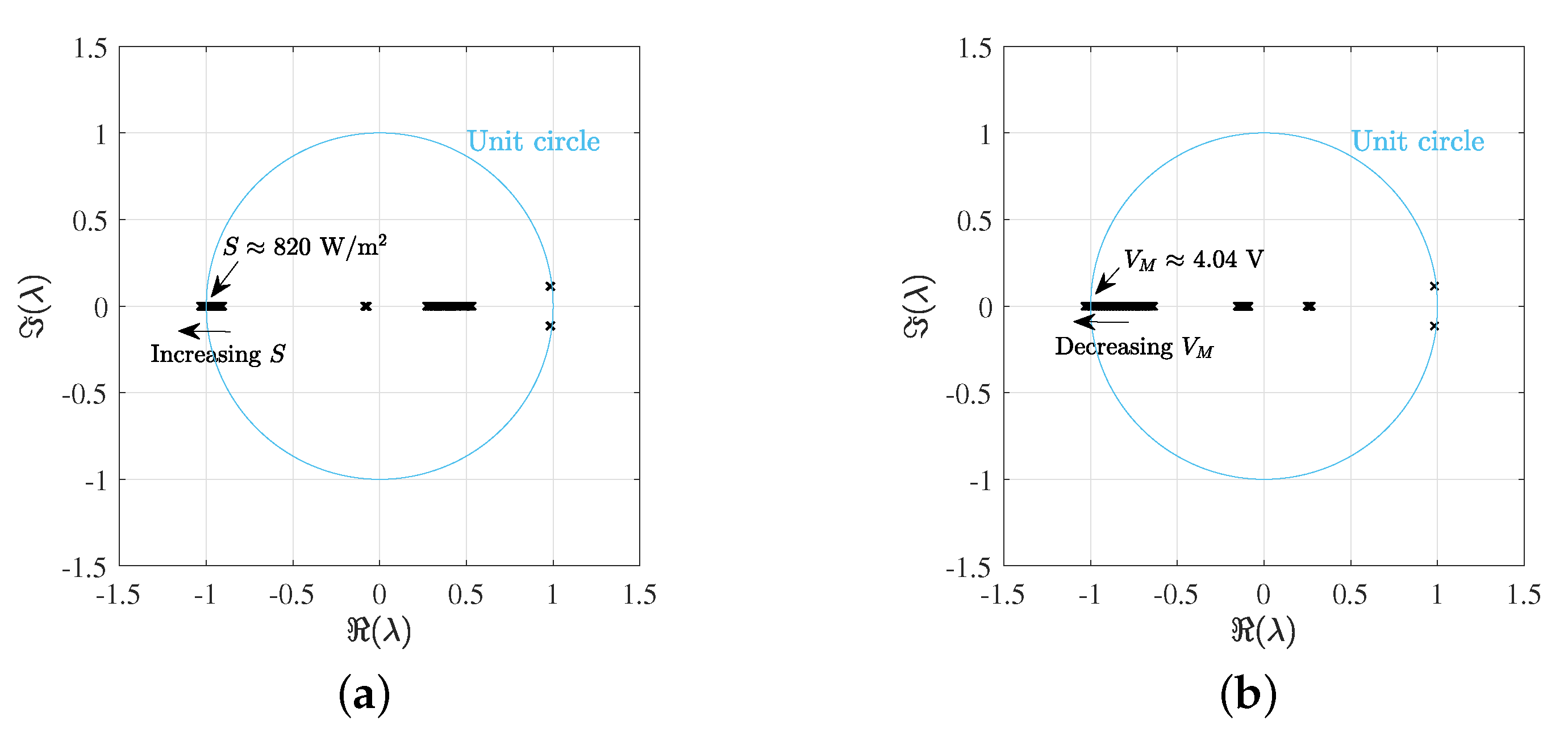
6.1. Stability Analysis of Periodic Orbits

The switching from the on to the off phase takes place whenever the ramp modulator signal $v_{\mathrm{ramp}}$ and the control signal $v_{\mathrm{con}}:=W_p{v}_p+W_i{v}_i$ intersect, i.e, whenever the following equality holds:

$$\begin{array}{ccc}\hfill W_i{v}_i\left(d_{n}T\right)+{\mathbf{K}}^{⊺}\mathbf{x}\left(d_{n}T\right)-v_{\mathrm{ramp}}\left(d_{n}T\right)& =& 0,\hfill \end{array}$$

(37)

where $\mathit{K}={(0,0,0,0,W_p)}^{⊺}$ is the vector of feedback gains and $d_n$ is the discrete-time the duty cycle during the $n^{\mathrm{th}}$ switching cycle. The steady-state value D of $d_n$ is imposed by the output DC-link voltage $V_{\mathrm{dcref}}$ and the MPP voltage $V_{\mathrm{mpp}}$. Therefore, for a fixed DC-link voltage $V_{\mathrm{dcref}}$, the steady-state duty cycle D is a function of the climatic conditions, and it is constrained by (16) with $V_{\mathrm{mpp}}$ as a function of the temperature $\mathrm{\Theta }$ and the irradiance S.

To perform a stability analysis of the system, Floquet theory is used and therefore the monodromy matrix $\mathbf{M}$ is first obtained. Let $\mathbf{x}\left(DT\right)={(\mathbf{I}-\mathrm{\Phi })}^{-1}\mathrm{\Psi }$ be the steady-state value of $\mathbf{x}\left(t\right)$ at time instant $DT$, where $\mathrm{\Phi }={\mathrm{\Phi }}_1{\mathrm{\Phi }}_0$, ${\mathrm{\Phi }}_1=e^{{\mathbf{A}}_{1}DT}$, ${\mathrm{\Phi }}_0=e^{{\mathbf{A}}_0(1-D)T}$, ${\mathrm{\Psi }}_1={(e^{{\mathbf{A}}_{1}DT}-\mathbf{I})}^{-1}\mathbf{B}\mathbf{w}$, ${\mathrm{\Psi }}_0={(e^{{\mathbf{A}}_0(1-D)T}-\mathbf{I})}^{-1}\mathbf{B}\mathbf{w}$, $\mathrm{\Psi }={\mathrm{\Phi }}_1{\mathrm{\Psi }}_0+{\mathrm{\Psi }}_1$. Let $m_a=V_M/T$ be the slope of the ramp-modulating signal, where $V_M$ is its peak-to-peak value. Let ${\mathit{m}}_1\left(\mathbf{x}\left(t\right)\right)={\mathbf{A}}_1\mathbf{x}\left(t\right)+{\mathbf{B}}_1\mathbf{w}$ and ${\mathit{m}}_0\left(\mathbf{x}\left(t\right)\right)={\mathbf{A}}_0\mathbf{x}\left(t\right)+{\mathbf{B}}_0\mathbf{w}$. Then, the monodromy matrix can be expressed as follows [22]:

$$\begin{array}{c}\hfill \mathbf{M}={\mathrm{\Phi }}_0\mathbf{S}{\mathrm{\Phi }}_1,\end{array}$$

(38)

where $\mathit{S}$ is the saltation matrix given by:

$$\begin{array}{c}\hfill \mathbf{S}=\mathbf{I}+{\displaystyle \frac{({\mathbf{m}}_0\left(\mathbf{x}\left(DT\right)\right)-{\mathbf{m}}_1\left(\mathbf{x}\left(DT\right)\right)){\mathbf{K}}^{⊺}}{W_i{v}_i\left(DT\right)+{\mathbf{K}}^{⊺}{\mathbf{m}}_1\left(\mathbf{x}\left(DT\right)\right)-m_a}}.\end{array}$$

(39)

Once the MPP voltage is obtained by maximizing the PV power, the steady-state duty cycle D is determined according to (16). The expression of $v_i\left(DT\right)$ that appears in (39) can be obtained from (37) in steady-state:

$$\begin{array}{c}\hfill v_i\left(DT\right)={\displaystyle \frac{1}{W_i}}({\mathbf{K}}^{⊺}\mathbf{x}\left(DT\right)-m_{a}DT)\end{array}$$

(40)

The study is done by using the set of parameter values of Table 3 for the quadratic boost converter and those shown in Table 1 for the PV module. First, $\mathbf{x}\left(DT\right)$ and $\mathbf{x}\left(0\right)$ are calculated, and the stability of the system is checked by observing the location of the eigenvalues of the monodromy matrix in the complex plane. Figure 12a shows the loci of these eigenvalues when the irradiance S is varied in the range $(500,1000)$$\mathrm{W}/{\mathrm{m}}^2$ for $V_M=4\mathrm{V}$. It can be observed that as the irradiance is increased above a critical value of $S\approx 820$$\mathrm{W}/{\mathrm{m}}^2$, the system undergoes a period doubling because one eigenvalue of the monodromy matrix leaves the unit disk from the point (−1,0). This explains the exhibition of the subharmonic oscillation observed previously in the time-domain waveforms of Figure 9a and Figure 10b and in the bifurcation diagrams of Figure 11. Note that the critical value predicted by the eigenvalues of the monodromy matrix is very close to the one predicted by the bifurcation diagram in Figure 11a. In turn, by fixing the irradiance S and the varying the amplitude $V_M$ of the ramp voltage $v_{\mathrm{ramp}}$, the same phenomenon is observed when $V_M$ is decreased. The variation of other parameters also leads to the exhibition of the same phenomenon whenever the operation in CCM is guaranteed.

Remark 2.

It can be observed that when the parameter values vary, only the eigenvalues of the monodromy located at the real axis move, while the complex conjugate ones remain practically constant and are maintained inside the unit disk. Therefore, the system does not undergo a slow-scale instability. This is due to the imposition of the LFR behavior at the input port of the converter, as already mentioned before. This is particularly important for a PV system since the optimum conductance $G_{\mathrm{mpp}}$ is constantly changed by the MPPT controller and the damping of the undesired oscillations caused by this change is better than in other control strategies, such as in [14,27].

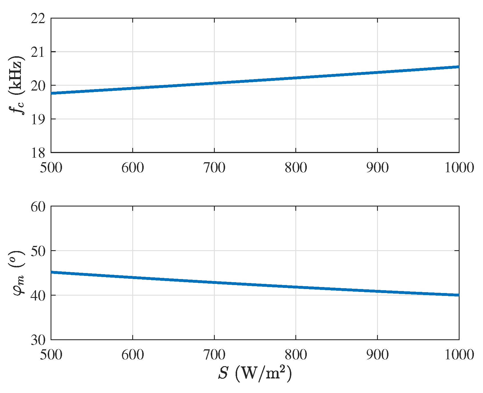
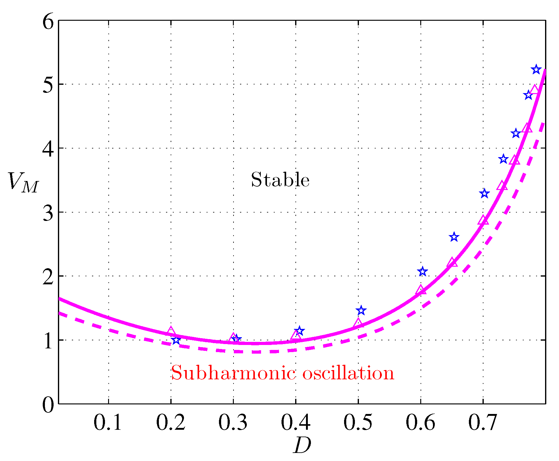
6.2. Analytical Determination of the Subharmonic Instability Boundaries

It was demonstrated in [35] that at the onset of subharmonic instability for a single-switch DC-DC regulator working in CCM, the following equality holds (The sign convention of the feedback coefficients has been adapted from [35]):

$$\begin{array}{c}\hfill m_a={\mathbf{K}}^{⊺}{(\mathbf{I}+\mathrm{\Phi })}^{-1}{\mathrm{\Phi }}_1({\mathbf{m}}_1\left(\mathbf{x}\left(0\right)\right)+{\mathbf{m}}_0\left(\mathbf{x}\left(0\right)\right))+m_i,\end{array}$$

(41)

where $\mathbf{x}\left(0\right)={(\mathbf{I}-\overline{\mathrm{\Phi }})}^{-1}\overline{\mathrm{\Psi }}$, $\overline{\mathrm{\Phi }}={\mathrm{\Phi }}_0{\mathrm{\Phi }}_1$, $\overline{\mathrm{\Psi }}={\mathrm{\Phi }}_0{\mathrm{\Psi }}_1+{\mathrm{\Psi }}_0$, and $m_i=W_i(G_{\mathrm{mpp}}{v}_{\mathrm{vp}}\left(DT\right)-i_{L1}\left(DT\right))$. The terms $v_{\mathrm{vp}}\left(DT\right)$ and $i_{L1}\left(DT\right)$ can be extracted from $\mathbf{x}\left(DT\right)$ defined previously. The theoretical results from expression (41) will be presented together with those corresponding to computer simulations and experimental results.

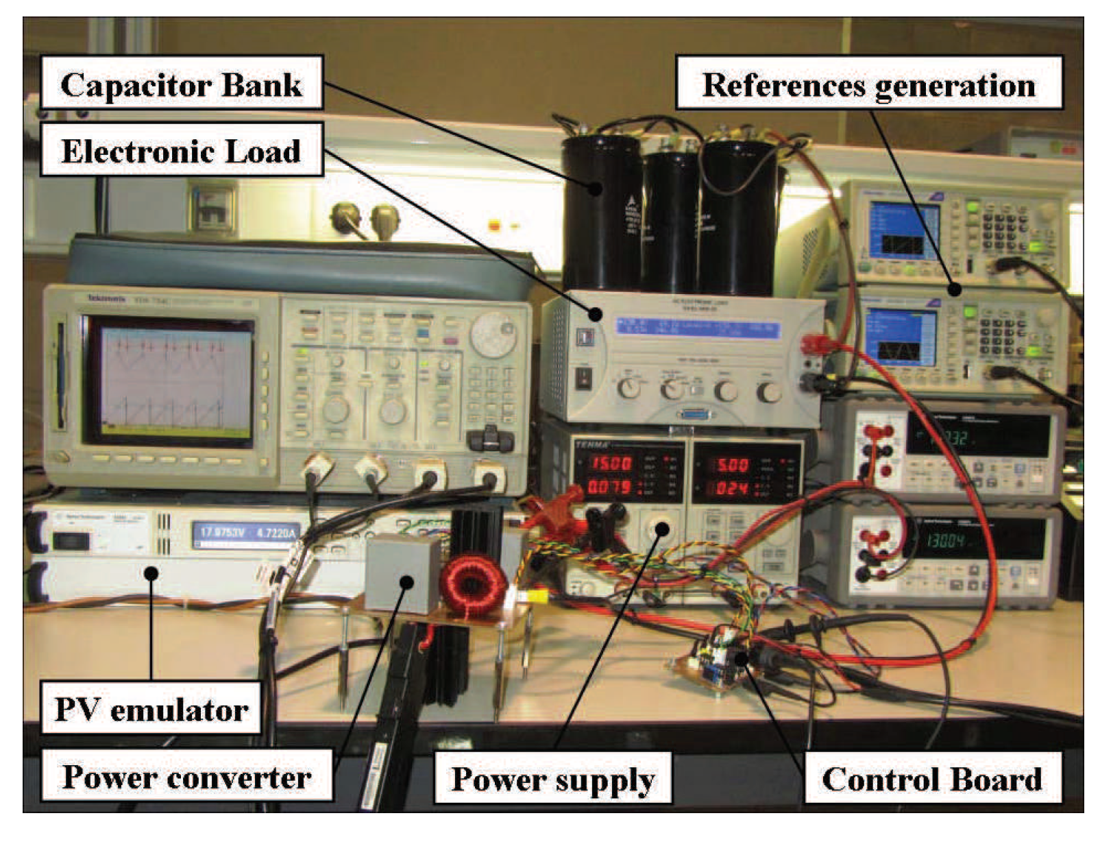
7. Validation of the Theoretical Results by Using Numerical Simulations and Experimental Results

To verify the theoretical and the time-domain simulation results, a DC-DC quadratic boost prototype was designed and implemented (Figure 13). In order to simplify the experimental setup and to obtain repeatable experiments, the PV emulator was used rather than a real PV generator. The main conclusions can be translated to real PV modules under the same weather conditions. An electronic active load was programmed in constant voltage mode and was connected at the output of the quadratic boost regulator with a type-II controller at the input side. A bank of capacitors of $28.2$ mF was connected between the converter and the active load to fix the output voltage.

The inductances have been built in-house and had the same nominal values as the ones used in the numerical simulations presented previously, i.e., $L_1^{*}=$138 $\mathsf{\mu }$H and $L_2^{*}=$5.5 mH. The input capacitor of 10 $\mathsf{\mu }$F was a metallized polyester capacitor (MKT) technology, and its rated voltage was 63 V. The intermediate and output capacitors of 10 $\mathsf{\mu }$F were metalized polypropylene film technology (MKP), and their rated voltage was 560 V. The power MOSFET (SIHG22N60E-GE3), with a rated voltage of 600 V, was used as a controlled switch of the quadratic boost regulator. The silicon carbide Schottky diodes (C3D10065A CREE) with a maximum reverse voltage VRRM voltage of 650 V were the diodes. The current sensing was performed by means of shunt resistors of 20 m$\mathrm{\Omega }$. Operational amplifiers MC33078 were used to amplify the sensed current. The analog multiplier (AD633JNZ) was used to obtain the reference current. The current error is processed by a PI controller with a tunable proportional gain. The output of the PI controller was followed by a low-pass filter hence obtaining the type-II controller. Like in the numerical simulations, the cut-off frequency of the low-pas filter was at one half the switching frequency (25 kHz). Note that a type-II controller is equivalent to a PI compensator cascaded with a low-pass filter. The same switching logic used in numerical simulations was used in the experimental prototype.

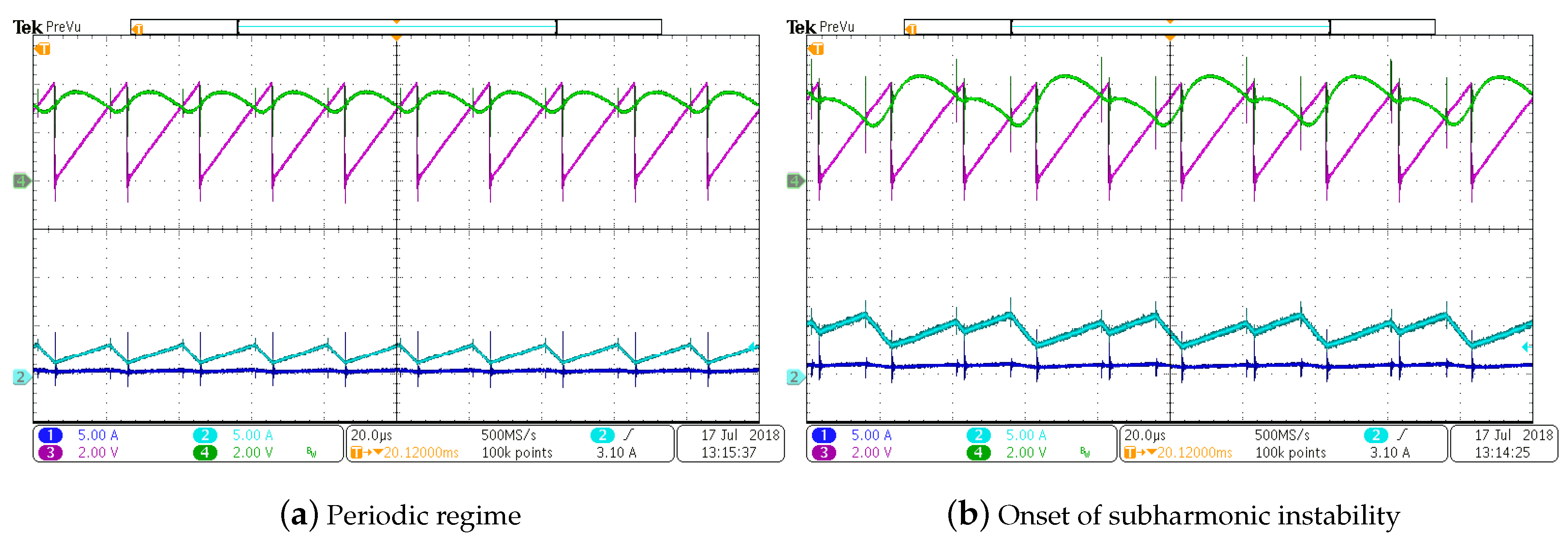
7.1. Experimental Test 1

To validate the numerical simulations experimentally, first, the experimental system response corresponding to Figure 9 was obtained from the laboratory prototype, and the results are depicted in Figure 14. The step change in the irradiance level was from 500 $\mathrm{W}/{\mathrm{m}}^2$–1000 $\mathrm{W}/{\mathrm{m}}^2$. First, for $S=$ 500 $\mathrm{W}/{\mathrm{m}}^2$, the system worked in the stable periodic regime. For $S=$ 1000 $\mathrm{W}/{\mathrm{m}}^2$, the subharmonic oscillation was exhibited. As can be observed, a close agreement between the numerical simulations in Figure 9 and the experimental measurements in Figure 14 was obtained.

To validate the previous methodology, the ramp signal amplitude $V_M$ was fixed in a relatively large value and then decreased till observing subharmonic instability at the oscilloscope screen, and the critical value of the ramp amplitude was recorded for several values of the operating duty cycle D in the range (0.2, 0.8). The duty cycle was varied by sweeping the active load voltage while maintaining the operation of the system at the MPP by selecting the suitable value of the conductance $g^{*}$ to be equal to the optimum value $G_{\mathrm{mpp}}=I_{\mathrm{mpp}}/V_{\mathrm{mpp}}$. Figure 15 shows the subharmonic instability boundary in the plane ($D,V_M$) obtained from (41) (dashed curve) using the values of inductances corresponding to no loading conditions and by experimental measurements (☆). A small discrepancy between the results can be observed. For instance, for $V_{\mathrm{dcref}}=$ 380 V, i.e, $D=0.7824$, the critical value of the ramp voltage amplitude from the theoretical expression was $V_M\approx 4.8$ V, while the one from the experimental measurements was $V_M\approx 5.2$ V. This mismatching between the theoretical and the experimental results can be attributed to many parasitic factors and non-modeled effects. However, it was observed that partial saturation of the inductors and the drop of their inductance values with the operating currents [41], is the main factor. Next, the saturability of the inductors will be taken into account. The variation of the inductance values versus their operating DC currents was experimentally determined.

An LCR meter and a current source, both controlled by a LabView^© software program, were used to measure the values of the inductances for different current levels. The experimental data obtained and a regression analysis based on least squared error revealed that in the range of current values used, the following linear expressions, relating the inductances $L_1$ and $L_2$ and their currents, can be used:

$$L_1\approx L_1^{*}-{\sigma }_1{I}_{L1},L_2\approx L_2^{*}-{\sigma }_2{I}_{L2},$$

(42)

where $L_1^{*}=138$ $\mathsf{\mu }$H and $L_2^{*}=5.5$ mH are the inductance values under no load condition, ${\sigma }_1=3$ $\mathsf{\mu }$H/A, ${\sigma }_2=1.2$ mH/A, and $I_{L1}$ and $I_{L2}$ are given by (14). The previous equations were used in both the theoretical expression (41) and in the numerical results. The theoretical results from (41) are depicted in Figure 15 in the solid curve and those from numerical simulations using PSIM^© software are indicated by △. After taking into account the inductances drop with the inductor current, a remarkable agreement among the experimental, theoretical and numerical results was obtained.

The waveforms of the inductor currents $i_{L1}$ and $i_{L2}$ at both sides of the subharmonic instability boundary are represented in Figure 16 together with the ramp signal and the control voltage. By comparing the waveforms in this figure and those in Figure 10, one can observe a good agreement between the measured and the simulated system dynamics.

7.2. Experimental Test 2

In this test, the output voltage was fixed at $V_{\mathrm{dcref}}=$ 380 V, the ramp signal peak-to-peak value was fixed at $V_M=4$ V, and the dynamics of the quadratic boost converter was explored by varying parameters corresponding to temperature and irradiance. Figure 17 shows the subharmonic instability boundary in the plane ($\mathrm{\Theta },S$) obtained from (41) while maintaining the PV emulator at its MPP. The four parameters needed to define the PV curve in this emulator were adjusted to different values to correspond to a temperature variation between 10 ${}^{\circ }$C and 70 ${}^{\circ }$C. The stability boundary is depicted in Figure 17. In this figure, the theoretical boundary obtained using (41) with fixed values of the inductances represented by the thin curve (upper) and experimental measurements are depicted. A significant mismatching can be observed between the results obtained by using the mathematical expression (41) with fixed values of inductances and the experimental measurements. The subharmonic instability boundary from numerical simulations (△) and from (41) (thick curve) by updating the inductances values according to (42) in both cases is also shown in Figure 17. Taking into account the inductances’ variation with the operating current, the agreement between the results is remarkable.

8. Conclusions

This study has shown that a high-voltage-gain DC-DC quadratic boost power converter connected to a grid-interlinked inverter in a PV system may undergo subharmonic instability when parameters such as those relayed to climatic conditions, loading and control circuit vary. The boundary of this instability has been located accurately using an analytical expression. Experimental tests, carried out using a laboratory prototype and numerical simulations from the switched model of the system, have been used to validate the theoretical derivations. The study provides a methodology for control-oriented modeling, nonlinear analysis and analytical determination of subharmonic instability boundary of energy conversion circuits used in PV systems. The presented methodology could help in tuning the different parameter values in order to avoid the undesired subharmonic oscillation, particularly as nonlinearity and/or parameter variations can be taken into account in the approach used. From a design perspective, the average small-signal model of the system can be used to achieve the desired performances in terms of stability phase margin, crossover frequency and settling time. However, subharmonic instability cannot be predicted by using this approach. Then, as a second step in the design, one should take into account the boundary condition given in this study to avoid problems related to subharmonic instability. In particular, the switching regulator control parameters such as the amplitude of the ramp modulator or the gain of the controller can be tuned according to the operating point in order to avoid the jeopardizing effects of such instability problems. These parameters must be tuned based on the highest irradiance level.

References

1. Fahimi, B.; Kwasinski, A.; Davoudi, A.; Balog, R.S.; Kiani, M. Powering a more electrified planet. IEEE Power Energy Mag. 2011, 54–64. Available online: https://www.ieee-pes.org/images/files/pdf/2012-pe-smart-grid-compendium.pdf (accessed on 28 December 2018).
2. Grubišić-Čabo, F.; Nizetić, S.; Giuseppe Marco, T. Photovoltaic panels: A review of the cooling techniques. Trans. Famena 2016, 40, 63–74. [Google Scholar]
3. Erickson, R.; Maksimovic, D. Fundamentals of Power Electronics, 2nd ed.; Kluwer Academic/Plenum Publishers: New York, NY, USA, 2001. [Google Scholar]
4. Alajmi, B.N.; Ahmed, K.H.; Finney, S.J.; Williams, B.W. A maximum power point tracking technique for partially shaded photovoltaic systems in microgrids. IEEE Trans. Ind. Electron. 2013, 60, 1596–1606. [Google Scholar] [CrossRef]
5. Sahan, B.; Vergara, A.N.; Henze, N.; Engler, A.; Zacharias, P. A single-stage PV module integrated converter based on a low-Power current-source inverter. IEEE Trans. Ind. Electron. 2008, 55, 2602–2609. [Google Scholar] [CrossRef]
6. Xiao, W. Photovoltaic Power System: Modelling, Design and Control; John Wiley & Sons: Hoboken, NJ, USA, 2017. [Google Scholar]
7. Wijeratne, D.S.; Moschopoulos, G. Quadratic power conversion for power electronics: Principles and circuits. IEEE Trans. Circuits Syst. I Regul. Pap. 2012, 59, 426–438. [Google Scholar] [CrossRef]
8. Lopez-Santos, O.; Martinez-Salamero, L.; Garcia, G.; Valderrama-Blavi, H.; Sierra-Polanco, T. Robust sliding-mode control design for a voltage regulated quadratic Boost Converter. IEEE Trans. Power Electron. 2015, 30, 2313–2327. [Google Scholar] [CrossRef]
9. Chen, Z.; Yang, P.; Zhou, G.; Xu, J.; Chen, Z. Variable duty cycle control for quadratic boost PFC converter. IEEE Trans. Ind. Electron. 2016, 63, 4222–4232. [Google Scholar] [CrossRef]
10. Langarica-Cordoba, D.; Diaz-Saldierna, L.H.; Leyva-Ramos, J. Fuel-cell energy processing using a quadratic boost converter for high conversion ratios. In Proceedings of the IEEE 6th International Symposium on Power Electronics for Distributed Generation Systems (PEDG), Aachen, Germany, 22–25 June 2015; pp. 1–7. [Google Scholar]
11. Deivasundari, P.S.; Uma, G.; Poovizhi, R. Analysis and experimental verification of Hopf bifurcation in a solar photovoltaic powered hysteresis current-controlled cascaded-boost converter. IET Power Electron. 2013, 6, 763–773. [Google Scholar] [CrossRef]
12. El Aroudi, A. Prediction of subharmonic oscillation in a PV-fed quadratic boost converter with nonlinear inductors. In Proceedings of the IEEE International Symposium on Circuits and Systems (ISCAS), Florence, Italy, 27–30 May 2018; pp. 1–5. [Google Scholar]
13. Valderrama-Blavi, H.; Bosque, J.M.; Guinjoan, F.; Marroyo, L.; Martinez-Salamero, L. Power adaptor device for domestic DC microgrids based on commercial MPPT inverters. IEEE Trans. Ind. Electron. 2013, 60, 1191–1203. [Google Scholar] [CrossRef]
14. Femia, N.; Petrone, G.; Spagnuolo, G.; Vitelli, M. Optimization of perturb and observe maximum power point tracking method. IEEE Trans. Power Electron. 2005, 20, 963–973. [Google Scholar] [CrossRef] [Green Version]
15. Banerjee, S.; Verghese, G.C. (Eds.) Nonlinear Phenomena in Power Electronics: Attractors, Bifurcations Chaos, and Nonlinear Control; IEEE Press: New York, NY, USA, 2001. [Google Scholar]
16. Tse, C.K. Complex Behavior of Switching Power Converters; CRC Press: New York, NY, USA, 2003. [Google Scholar]
17. Cheng, L.; Ki, W.H.; Yang, F.; Mok, P.K.T.; Jing, X. Predicting subharmonic oscillation of voltage-mode switching converters using a circuit-oriented geometrical approach. IEEE Trans. Circuits Syst. I Regul. Pap. 2017, 64, 717–730. [Google Scholar] [CrossRef]
18. Lu, W.; Li, S.; Chen, W. Current-ripple compensation control technique for switching power converters. IEEE Trans. Ind. Electron. 2018, 65, 4197–4206. [Google Scholar] [CrossRef]
19. Islam, H.; Mekhilef, S.; Shah, N.B.M.; Soon, T.K.; Seyedmahmousian, M.; Horan, B.; Stojcevski, A. Performance Evaluation of maximum power point tracking approaches and photovoltaic systems. Energies 2018, 11, 365. [Google Scholar] [CrossRef]
20. Abusorrah, A.; Al-Hindawi, M.M.; Al-Turki, Y.; Mandal, K.; Giaouris, D.; Banerjee, S.; Voutetakis, S.; Papadopoulou, S. Stability of a boost converter fed from photovoltaic source. Sol. Energy 2013, 98, 458–471. [Google Scholar] [CrossRef]
21. Al-Hindawi, M.; Abusorrah, A.; Al-Turki, Y.; Giaouris, D.; Mandal, K.; Banerjee, S. Nonlinear dynamics and bifurcation analysis of a boost converter for battery charging in photovoltaic applications. Int. J. Bifurc. Chaos 2014, 24, 1450142. [Google Scholar] [CrossRef]
22. Giaouris, D.; Banerjee, S.; Zahawi, B.; Pickert, V. Stability analysis of the continuous-conduction-mode buck converter via Filippov’s method. IEEE Trans. Circuits Syst. I Regul. Pap. 2008, 55, 1084–1096. [Google Scholar] [CrossRef]
23. El Aroudi, A. Out of Maximum Power Point of a PV system because of subharmonic oscillations. In Proceedings of the International Symposium on Nonlinear Theory and Its Applications, NOLTA2017, Cancún, Mexico, 4–7 December 2017. [Google Scholar]
24. Lee, J.H.; Bae, H.S.; Cho, B.H. Resistive control for a photovoltaic battery charging system using a microcontroller. IEEE Trans. Ind. Electron. 2008, 55, 2767–2775. [Google Scholar] [CrossRef]
25. Valencia, P.A.O.; Ramos-Paja, C.A. Sliding-mode controller for maximum power point tracking in grid-connected photovoltaic systems. Energies 2015, 8, 12363–12387. [Google Scholar] [CrossRef]
26. Shmilovitz, D. On the control of photovoltaic maximum power point tracker via output parameters. IEE Proc. Electr. Power Appl. 2005, 152, 239–248. [Google Scholar] [CrossRef]
27. Xiao, W.; Ozog, N.; Dunford, W.G. Topology study of photovoltaic interface for maximum power point tracking. IEEE Trans. Ind. Electron. 2007, 54, 1696–1704. [Google Scholar] [CrossRef]
28. Bianconi, E.; Calvente, J.; Giral, R.; Mamarelis, E.; Petrone, G.; Ramos-Paja, G.C.A.; Spagnuolo, G.; Vitelli, M.M. A fast current-based MPPT technique employing sliding mode control. IEEE Trans. Ind. Electron. 2012, 60, 1168–1178. [Google Scholar] [CrossRef]
29. Huang, L.; Qiu, D.; Xie, F.; Chen, Y.; Zhang, B. Modeling and stability analysis of a single-phase two-stage grid-connected photovoltaic system. Energies 2017, 10, 2176. [Google Scholar] [CrossRef]
30. Rodrigues, E.M.G.; Godina, R.; Marzband, M.; Pouresmaeil, E. Simulation and Comparison of Mathematical Models of PV Cells with Growing Levels of Complexity. Energies 2018, 11, 2902. [Google Scholar] [CrossRef]
31. Villalva, M.; Gazoli, J.; Filho, E. Comprehensive approach to modeling and simulation of photovoltaic arrays. IEEE Trans. Power Electron. 2009, 24, 1198–1208. [Google Scholar] [CrossRef]
32. BP Solar BP585 Datasheet. Available online: http://www.electricsystems.co.nz/documents/BPSolar85w.pdf (accessed on 19 December 2018).
33. Krein, P.T.; Balog, R.S.; Mirjafari, M. Minimum energy and capacitance requirements for single-phase inverters and rectifiers using a ripple port. IEEE Trans. Power Electron. 2012, 27, 4690–4698. [Google Scholar] [CrossRef]
34. El Aroudi, A. A new approach for accurate prediction of subharmonic oscillation in switching regulators— Part II: Case studies. IEEE Trans. Power Electron. 2017, 32, 5835–5849. [Google Scholar] [CrossRef]
35. El Aroudi, A. A new approach for accurate prediction of Subharmonic oscillation in switching regulators— Part I: Mathematical derivations. IEEE Trans. Power Electron. 2017, 32, 5651–5665. [Google Scholar] [CrossRef]
36. Xiao, W.; Dunford, W.G.; Palmer, P.R.; Capel, A. Regulation of photovoltaic voltage. IEEE Trans. Ind. Electron. 2007, 54, 1365–1374. [Google Scholar] [CrossRef]
37. Al-Turki, Y.; El Aroudi, A.; Mandal, K.; Giaouris, D.; Abusorrah, A.; Al Hindawi, M.; Banerjee, S. Nonaveraged control-oriented modeling and relative stability analysis of DC-DC switching converters. Int. J. Circuit Theory Appl. 2018, 46, 565–580. [Google Scholar] [CrossRef]
38. Haroun, R.; El Aroudi, A.; Cid-Pastor, A.; Garcia, G.; Olalla, C.; Martinez-Salamero, L. Impedance matching in photovoltaic systems using cascaded boost converters and sliding-mode control. IEEE Trans. Power Electron. 2015, 30, 3185–3199. [Google Scholar] [CrossRef]
39. Leyva, R.; Alonso, C.; Queinnec, I.; Cid-Pastor, A.; Lagrange, D.; Martinez-Salamero, L. MPPT of photovoltaic systems using extremum-seeking control. IEEE Trans. Aerosp. Electron. Syst. 2006, 42, 249–258. [Google Scholar] [CrossRef]
40. Zhou, Y.; Tse, C.K.; Qiu, S.S.; Lau, F.C.M. Applying resonant parametric perturbation to control chaos in the buck DC/DC converter with phase shift and frequency mismatch considerations. Int. J. Bifurc. Chaos Appl. Sci. Eng. 2003, 13, 3459–3471. [Google Scholar] [CrossRef]
41. Di Capua, G.; Femia, N. A novel method to predict the real operation of ferrite inductors with moderate saturation in switching power supplies applications. IEEE Trans. Power Electron. 2016, 31, 2456–2464. [Google Scholar] [CrossRef]
Figure 1. A model of a PV-based DC microgrid equipped with high-voltage-gain MICs.
Energies 12 00061 g001
Figure 2. Two-stage grid connected PV system with a quadratic boost converter in the DC-DC stage.
Energies 12 00061 g002
Figure 3. The single-diode five-parameter equivalent circuit diagram of the PV generator according to (1) [31].
Energies 12 00061 g003
Figure 4. The BP585PV module i v characteristic and its linear approximation (dashed) at the MPP for S = 1000 W/m 2 and Θ = 25 C. The load line of the optimum conductance G mpp = 0.2524 S and the Norton equivalent conductance G p N = 0.35322 S are also shown.
Energies 12 00061 g004
Figure 5. The two simplified equivalent circuit configurations of the system of Figure 2 for the different switch S states where the PV generator is substituted by its linearized Norton equivalent and the grid-interlinked inverter is substituted by a constant DC voltage.
Energies 12 00061 g005
Figure 6. Equivalent block diagram of a type-II controller.
Energies 12 00061 g006
Figure 7. The crossover frequency f c (top) and the phase margin φ m (bottom) of the small-signal model of the quadratic boost converter with the input voltage control for different values of the irradiance S between 500 W / m 2 ( P max 42 W) and 1000 W / m 2 ( P max 85 W). V M = 4 V. Θ = 25 C.
Energies 12 00061 g007
Figure 8. The startup response of the quadratic boost converter with a nonlinear PV source under MPPT control S = 500 W / m 2 , V M = 4 V. Θ = 25 C.
Energies 12 00061 g008
Figure 9. The simulated PV system response to a change at t = 150 ms in the irradiance level from 500 W/m2 ( P max 42 W) to 1000 W/m2 ( P max 85 W). V M = 4 V. Θ = 25 C.
Energies 12 00061 g009
Figure 10. Close view of the ramp signal vramp, the control signal vcon, and the inductor currents iL1 and IL2 at the DC-DC stage.
Energies 12 00061 g010
Figure 11. The bifurcation diagram of the quadratic boost regulator with a nonlinear PV source under extremum seeking MPPT control for regulating the input voltage taking the irradiance S as a bifurcation parameter. (a) With the exact theoretical conductance g * and (b) with the conductance G mpp provided by the extremum seeking MPPT. V M = 4 V. Θ = 25 C.
Energies 12 00061 g011
Figure 12. Monodromy matrix eigenvalues’ loci for (a) the irradiance S ( 500 , 1000 ) W / m 2 , V M = 4 V , Θ = 25 C, and (b) the ramp peak-to-peak amplitude V M ( 4 , 5 ) V , S = 1000 W / m 2 , Θ = 25 C.
Energies 12 00061 g012
Figure 13. A picture of the experimental setup where the quadratic boost converter, the PV emulator, and the electronic load are used to obtain the experimental results.
Energies 12 00061 g013
Figure 14. The experimental PV system response due to a change of step type in the irradiance level from 500 W / m 2 –1000 W / m 2 as in Figure 9. V M = 4 V.
Energies 12 00061 g014
Figure 15. The stability boundary in the ( D , V M ) parameter space from the theoretical expression (41) by using fixed values of the inductances L 1 * = 138 μ H and L 2 * = 5.5 mH (dashed curve), by updating the inductances L 1 and L 2 values according to (42) (solid curve and △) and experimentally (☆).
Energies 12 00061 g015
Figure 16. Experimental waveforms of the quadratic boost converter fed by a PV generator before ( S = 500 W / m 2 ) and after S = 750 W / m 2 subharmonic oscillation takes place. V M = 4 V. Θ = 25 C. Other parameters’ values are from Table 3.
Energies 12 00061 g016
Figure 17. The subharmonic instability boundary in the parameter plane ( Θ , S ). The results are obtained from the theoretical expression (41) with L 1 and L 2 fixed (thin curve), with L 1 and L 2 varied according to (42) (thick curve), from computer simulations performed on the switched model with L 1 and L 2 varied according to (42) (△), and experimentally (⋆). V M = 4 V.
Energies 12 00061 g017