Fuzzy Damage Analysis of the Seismic Response of a Long-Distance Pipeline under a Coupling Multi-Influence Domain

Abstract

For a long-distance pipeline, the seismic load is a four-dimensional space-time excitation that simultaneously changes with time and space. In this work, a novel random space-time seismic model is established for a long-distance pipeline, which uses the Clough-Penzien model based on a random process and model of a random field. The response analysis of a long-distance pipeline for multipoint excitation and a buried pressure pipeline are established, while the stress analysis of the buried pressure pipeline is carried out in combination with von Mises theory. In addition, we consider the impact of the site type. The application of the proposed methodology is proved through numerical simulation. A fuzzy damage model and fuzzy safety criteria are established to assess the degree of the structure. The results indicate that a reasonable assessment and design method should consider the coupling multi-influence domain. In particular, evaluation of the structural damage should be done to establish fuzzy damage models and fuzzy safety criteria. The effective measurement of the uncertainty of such parameters forms an important basis for subsequent structural reliability analysis and design.

1. Introduction

Oil/gas use has increased with the increasing development of the world economy. For the transport infrastructure, pipelines are regarded as an important lifeline engineering component [1,2,3]. Over the past decade, the world has entered an era of frequent earthquakes. Therefore, the evaluation of pipelines should be treated as essential research. The ground motion of earthquakes is a nonstationary random process [4]. For a long-distance pipeline, structures with large spatial spans are not only affected by the time-varying characteristics of seismic loads but are also sensitive to the spatial correlation of seismic loads. With the development of the theory of the random process of ground motion, the research field has included objective analysis of the influencing factors. However, only the European seismic code has considered the spatial impact of the load, while the other standards have addressed the uniform excitation of a seismic load [5]. Under the effects of spatial ground motions, Novak and Hindy were the first to analyze the response analysis of structures statistically [6]. Until the array recording device was widely used, researchers studied the multipoint excitation response problem of large-span structures from a statistical point of view. The data recorded by the SMART-1 seismic array were used as a representative source to derive the spatial correlation of ground motion [7]. The time variation can be used in the theory of random process. The random process is an infinite dimensional random variable, which is significantly represented by a huge amount of computation in the analysis of ground motion. Although the classical representation Karhunen-Loeve decomposition generally requires a large number of random variables, the quadratic orthogonal expansion method uses approximately only 10 random variables to definite the random process of ground motion [8,9,10]. In addition, He et al. proposed a space–time influence domain to quantify the subsequence of earthquakes that were directly influenced by previous earthquakes [11]. To solve the uncertainty in safety evaluation, Zadeh proposed fuzzy set theory [12]. Some researchers have applied fuzzy logic to address the risk assessment for pipelines [13,14]. However, there is currently no fuzzy damage evaluation system for pipelines subjected to earthquakes.

In response to the limitations of research of pipelines exposed to earthquakes, this paper presents a methodology to couple the multi-influence domain of seismic factors. It puts forward an appropriate methodology to analyze the response of long-distance pipelines exposed to four-dimensional earthquakes. Based on the theory of random process and random fields, this paper establishes a model to apply in the design of pipeline engineering. Specifically, the construction procedure of the stochastic space-time seismic model is unified. In this way, numerical examples are investigated to prove the necessity of considering the space-time characteristics of a long-distance pipeline. Hence, the role of the impact of the local site owing to different site types is also presented. In addition, fuzzy damage criteria are established based on uncertainty theory. Based on the established model and assessment criteria, the safe evaluation system of a long-distance pipeline can be supplemented.

2. Ground Motion of the Random Field

The spatial variation of ground motion refers mainly to the coherence effect, traveling wave effect and site effect. The coherence effect is the loss of spatial coherence due to reflection and refraction in the propagation of seismic waves. Due to the different phases, frequencies in different structural locations and the different formation media, the influence on the structural response is affected. The traveling wave effect refers to the change of phase difference caused by a finite velocity of a seismic wave, which is essential to the response change of the time when the seismic wave arrives at each position of the structure with hysteresis. Local site effects refer to the effects of different soil properties on seismic waves. When the duration of seismic waves, the spectral characteristics of ground motions and the intensity of ground motions differ greatly, local site effects are particularly significant. Clearly, as for the long-distance structure, the response of the pipeline influences the random space.

2.1. Definition of Random Fields

According to the theory of random process, $(\mathsf{\Omega },\mathrm{P},\mathsf{\eta })$ is the probability space, and $T$ is a subset of the real number set. If $t\in T$, then $X(t,\omega )$ is a random variable in the probability space $(\mathsf{\Omega },\mathrm{P},\mathsf{\eta })$. Thus, the family of random variables $\left\{X(t,\omega ),t\in T\right\}$ is a random process on the probability space $(\mathsf{\Omega },\mathrm{P},\mathsf{\eta })$. Therefore, the random field can be defined such that the concept of a stochastic process is generalized in the spatial fields. When x is the spatial position, $H(x)$ is expressed as a random variable. Then, the random field is a random variable in the field parameter set [15].

2.2. Model of Random Fields

The power spectrum matrix of the spatial ground motion model is [16]

$$\left[S(\mathrm{i}{\omega }_{\mathrm{e}})\right]=[\begin{array}{l}{S}_{11}(\mathrm{i}{\omega }_{\mathrm{e}})\cdots S_{1\mathrm{n}}(\mathrm{i}{\omega }_{\mathrm{e}})\cdots \\ ⋮\\ S_{\mathrm{n}1}(\mathrm{i}{\omega }_{\mathrm{e}})\cdots S_{\mathrm{nn}}(\mathrm{i}{\omega }_{\mathrm{e}})\cdots \\ ⋮\\ S_{\mathrm{m}1}(\mathrm{i}{\omega }_{\mathrm{e}})\cdots S_{\mathrm{mn}}(\mathrm{i}{\omega }_{\mathrm{e}})\cdots \end{array}\begin{array}{l}{S}_{1\mathrm{m}}(\mathrm{i}{\omega }_{\mathrm{e}})\\ ⋮\\ S_{\mathrm{nm}}(\mathrm{i}{\omega }_{\mathrm{e}})\\ ⋮\\ S_{\mathrm{mm}}(\mathrm{i}{\omega }_{\mathrm{e}})\end{array}]$$

(1)

where $\left[S(\mathrm{i}{\omega }_{\mathrm{e}})\right]$ is the power spectrum matrix; $S_{ii}(\mathrm{i}{\omega }_{\mathrm{e}})$ is the power spectral density of the ground motion, which describes the frequency domain characteristics of ground motions at various points in the seismic field and the comparison of the frequency characteristics; and ${\omega }_{\mathrm{e}}$ is the earthquake frequency.

$$S_{\mathrm{mn}}(\mathrm{i}{\omega }_{\mathrm{e}})=\left|{\rho }_{\mathrm{mn}}\right|\exp (-\mathrm{i}{\omega }_{\mathrm{e}}\frac{d_{\mathrm{mn}}}{v})\sqrt{S_{\mathrm{mm}}(\mathrm{i}{\omega }_{\mathrm{e}})S_{\mathrm{nn}}(\mathrm{i}{\omega }_{\mathrm{e}})}$$

(2)

where $S_{\mathrm{mn}}(\mathrm{i}{\omega }_{\mathrm{e}})$ is seismic power spectral density of the two points m and n; $\left|{\rho }_{\mathrm{mn}}\right|$ is the partial coherence effect, with $\left|{\rho }_{\mathrm{mn}}\right|\le 1$; $\exp (-\mathrm{i}{\omega }_{\mathrm{e}}\frac{d_{\mathrm{mn}}}{v})$ is the traveling wave effect; $d_{\mathrm{mn}}$ is the distance between m and n; and $v$ is the speed of the visual wave.

2.3. Pipeline Random Field Model Based on Statistical Data

The random field is the process of spatial variation of the ground motion. In recent years, with the increase of observation arrays for recording strong earthquakes, researchers have proposed to use statistical regression to obtain the coherence function model to express the random field of ground motion [17,18].

Under the frequency domain, we can introduce a coherence function to definite the spatial coherence degree of the two points A and B, which is defined as follows:

$${\gamma }_{\mathrm{AB}}({\omega }_{\mathrm{e}})=\left|\frac{S_{\mathrm{AB}}({\omega }_{\mathrm{e}})}{\sqrt{S_{\mathrm{AA}}({\omega }_{\mathrm{e}})S_{\mathrm{BB}}({\omega }_{\mathrm{e}})}}\right|\exp \left[-i{\theta }_{\mathrm{AB}}({\omega }_{\mathrm{e}})\right]$$

(3)

where ${\gamma }_{\mathrm{AB}}(d,\omega )$ is the coherence function; $S_{\mathrm{AB}}({\omega }_{\mathrm{e}})$ is the cross-power spectrum of A and B; $S_{\mathrm{AA}}({\omega }_{\mathrm{e}})$ and $S_{\mathrm{BB}}({\omega }_{\mathrm{e}})$ are the self-power spectrum of two points A and B, respectively; and ${\theta }_{\mathrm{AB}}({\omega }_{\mathrm{e}})$ is the coherence angle of the traveling wave effect for A and B.

The coherence function of the ground motion is obtained by the self-power spectrum standardization of the cross-power spectrum between two points of the structure [19]. The majority of the coherence functions are based on the earthquake statistics records obtained by the earthquake station. Moreover, these data can be generally divided into empirical coherence models, theoretical coherence models and semiempirical semitheoretical coherence models.

This paper proposes the semitheoretical semiempirical coherent model proposed by Luco and Wong, which features universality and is the most widely used [20]:

$${\gamma }_{\mathrm{p}}({\omega }_{\mathrm{e}},d)=\exp \left[-{\alpha }^2{{\omega }_{\mathrm{e}}}^2{d}^2\right]$$

(4)

where ${\gamma }_{\mathrm{p}}({\omega }_{\mathrm{e}},d)$ is the semitheoretical semiempirical coherence function; $\alpha$ is the coherent attenuation parameter, with (2 − 3) × 10⁻⁴ s in the current study; and $d$ is the distance between any two points.

The damped natural vibration frequency of the long-distance pipeline in this paper has the following form:

$${\omega }_{\mathsf{\xi }}=\sqrt{\frac{\overline{k}}{\overline{m}}+\frac{n^2{\mathsf{\pi }}^{2}K}{l^2\overline{m}}(1-{\xi }_i)},(i=0,1,2,3\dots n)$$

(5)

where ${\omega }_{\mathsf{\xi }}$ is the damped frequency of the pipeline; $\overline{m}$ is the weight of the pipeline per unit length; $\overline{k}$ is the stiffness coefficient around the pipeline per unit length; $K$ is the axial stiffness of the pipeline; l is the length of the pipeline; and ${\xi }_i$ is the damping ratio of the i-th vibration type.

3. Random Process of Ground Motion

3.1. Definition of a Nonstationary Earthquake Random Process

According to the statistical data, the random process is divided into a stationary random process and a nonstationary random process. A one-dimensional random process can be regarded as a generalization of multiple random variables. Thus, when the dimension of a multivariate random variable is a parameter, the time parameter of a one-dimensional random process is the result of a continuous change. The statistical features of earthquake action change with time. In addition, strong ground motion is a nonstationary process with transient time. For the nonstationary random process of earthquake loads, researchers typically use a deterministic intensity function that varies over time and a stationary random process to reflect the nonstationarity.

In the view of statistics, the autocorrelation function is defined as the Pearson’s correlation between the values at different times of a random process. This parameter is a signal of the reflexive cross-correlation at different time points or a function of the time difference between pairs of similarity between two observations. Since the autocorrelation function of the stationary stochastic process is equivalent to the auto spectral density about the information of the process, the spectral density can be defined from the Fourier transform representation theorem of the autocorrelation function. The spectral density represents the statistical information about the amplitude of the random process in the frequency fields. The equation of spectral density proposed by Wiener and Khintchine according to the Fourier transformation [21] is

$$S_x(\omega )=\frac{1}{2\mathsf{\pi }}{\displaystyle {\int }_{-\infty }^{\infty }{R}_x}(\tau )\exp (-\mathrm{i}\omega \tau )\mathrm{d}\tau$$

(6)

$$R_x(\tau )={\displaystyle {\int }_{-\infty }^{\infty }{S}_x}(\omega )\exp (\mathrm{i}\omega \tau )\mathrm{d}\omega$$

(7)

Assuming $\tau =0$,

$$R_x(0)=\mathrm{E}\left[x^2(t)\right]={\displaystyle {\int }_{-\infty }^{\infty }{S}_x}(\omega )\mathrm{d}\omega ={\sigma }^2$$

(8)

where $S_x(\omega )$ is the self-power spectral density function; $R_x(\tau )$ is the autocorrelation function; i is the virtual unit; $\tau$ is the time equation; ω is the frequency of vibration, with $\omega \in (-\infty ,+\infty )$; $x(t)$ is the self-power spectral density function; t is time, with $t\in (0,+\infty )$; and ${\sigma }^2$ is the mean square value of $x(t)$.

However, when the actual waveform x(t) is as the object, the relationship of $S_x(\omega )$ and $G_x(\omega )$ are shown in Figure 1, and the self-power spectral density function $G_x(\omega )$ in the positive number domain has the following expression:

$$S_x(\omega )=2G_x(\omega )$$

(9)

3.2. Random Process Model of Ground Motion and Its Orthogonal Development

3.2.1. Random Process Model of Ground Motion

Among the random ground motion models, the Kanai-Tajimi power spectral density model is the most representative, and various models are modified from it. Although the classical Kanai-Tajimi model has an explicit physical meaning, it exaggerates the energy of low-frequency ground motion. In addition, it does not satisfy the bounded conditions of ground motion.

Subsequently, many scholars have revised the Kanai-Tajimi model. The most widely used is the Clough-Penzien model of the random ground motion power spectrum, which is proposed as follows [22]:

$$S_{\mathrm{cp}}(\omega )=\frac{{\omega }_{\mathrm{g}}^4{\omega }^4+4{\xi }_{\mathrm{g}}^2{\omega }_{\mathrm{g}}^2{\omega }^6}{\left[{({\omega }^2-{\omega }_{\mathrm{f}}^2)}^2+4{\xi }_{\mathrm{f}}^2{\omega }_{\mathrm{f}}^2{\omega }^2\right]\left[{({\omega }^2+{\omega }_{\mathrm{g}}^2)}^2+4{\xi }_{\mathrm{g}}^2{\omega }_{\mathrm{g}}^2{\omega }^2\right]}{S}_0$$

(10)

where $S_0$ is the spectral density of Gaussian white noise (filter input) with mean 0; ${\omega }_{\mathrm{g}}$ is the characteristic frequency of the site; ${\xi }_{\mathrm{g}}$ is the damping ratio of the characteristic site; ${\omega }_{\mathrm{f}}$ is the site characteristic frequency of low-frequency filtering; and ${\xi }_{\mathrm{f}}$ is the characteristic damping ratio of low-frequency filtering.

3.2.2. Orthogonal Expansion of Random Processes of Ground Motion

In practical engineering, there are mostly random dynamic loads. Therefore, many random phenomena need to be described by random processes. The rational use of the power spectral density function to analyze the random process of ground motions is mathematically within the scope of numerical characteristics. Thus, it is challenging to intuitively reflect the certainty of the power spectral density function and the random process sample. In the essential point of view, the random process is a method of efficient data compression and extraction of the essential features of the random process. For continuous stochastic functions, the Karhunen-Loeve (K-L) decomposition provides a class of integral spectrum operators. Based on the standard orthogonal basis of random process expansion method, the basic guideline is to describe the random process as a linear combination of deterministic functions modulated by a small number of uncorrelated random coefficients [4]. The K-L decomposition generally requires a large number of random variables to describe the random process, while the orthogonal expansion of the Hartley orthogonal basis for a random process use only a small number of independent random variables, which reflects the complex random process probabilistic characteristics of ground motion.

The K-L decomposition of random processes describes the random process as a linear combination of deterministic functions described by mutually independent random coefficients. This approach provides a study of random processes from the independent set of random variables [23]. The main purpose of the K-L decomposition is to characterize the main energy coherent structure of the random process with only a small amount of expansion terms.

The K-L decomposition is defined in the probability space $(x,y,z)$ and the bounded interval’s real-valued random process $u(\theta ,x)$. For any $x\in D$, the mean function is $\overline{u}(x)$, and the finite variance $E{\left[u(\theta ,x)-\overline{u}(x)\right]}^2$ is bounded. Thus, the random process $u(\theta ,x)$ can be expressed as

$$u(\theta ,x)=\overline{u}(x)+{\displaystyle \sum _{i=1}^{\infty }\sqrt{{\lambda }_i}}{\xi }_i(\theta )f_i(x)$$

(11)

where $u(\theta ,x)$ is a stochastic process; $\overline{u}(x)$ is the mean function; ${\lambda }_i$ is the eigenvalue of the covariance function $C(x_1,x_2)$ for the random process $u(\theta ,x)$; $f_i(x)$ is the characteristic function of the covariance function $C(x_1,x_2)$ for the random process $u(\theta ,x)$; and $x_1$ and $x_2$ are variables.

According to Mercer’s theorem, the covariance function of a random process can be decomposed into the following:

$$C(x_1,x_2)={\displaystyle \sum _{i=1}^{\infty }{\lambda }_i{f}_i(x_1)f_i(x_2)}$$

(12)

where $C(x_1,x_2)$ is the covariance function and $f_i(x_1)$ and $f_i(x_2)$ are characteristic functions of variable $x_i$.

${\lambda }_i$ and $f_i(x)$ can be obtained by the integral equation of Fredholm:

$${\displaystyle {\int }_{D}C(x_1,x_2)}{f}_i(x_1)d{x}_1={\lambda }_i{f}_i(x_2)$$

(13)

3.3. Orthogonal Expansion of the Clough-Penzien Model Based on an Orthonormal Basis

With the study of probabilistic features, the random expansion based on the standard orthogonal basis is intended to reflect the random process with a small number of random variables. The form of the C-P model is equivalent to K-L decomposition.

This paper uses the spectral density function of the C-P model for ground motion, whose values of parameters are shown in

Table 1. Intensity factor of the C-P model spectrum.

Site Category	Spectral Intensity Factor S0	Peak Factor f	ωe	Maximum Acceleration ${\overline{\mathit{a}}}_{\max }$
Hard soil site	54.14	3.0	78.84	196 (0.2 g)
Medium soil site	81.15	3.1	49.26	196 (0.2 g)
Weak soil site	145.98	3.2	25.70	196 (0.2 g)

and

Table 2. Values of C-P model parameters [24,25].

Site Category	ωg	ωf	ξg	ξf
Hard soil site	8π	0.8π	0.60	0.60
Medium soil site	5π	0.5π	0.60	0.60
Weak soil site	2.4π	0.24π	0.85	0.85

, and the corresponding autocorrelation function is

$$R_x(\tau )=S_0\mathsf{\pi }{\displaystyle \sum _{i=1}^4{A}_i(\tau )}$$

(14)

where $A_i(\tau )$ is the i-th orthogonal expansion term, with $i=1,2,3,4$.

Thus, the expression $A_i(\tau )$ can be expressed as

$$A_1(\tau )=\frac{{\omega }_{\mathrm{g}}^4+4{\xi }_{\mathrm{g}}^2{\omega }_{\mathrm{g}}^2{\omega }_1^2}{({\omega }_1-{\omega }_2)({\omega }_1-{\omega }_3)({\omega }_1-{\omega }_4)}\times \frac{\exp (\mathrm{i}\left|\tau \right|{\omega }_1)}{{({\omega }_1^2-{\omega }_{\mathrm{f}}^2)}^2+4{\xi }_{\mathrm{f}}^2{\omega }_{\mathrm{f}}^2{\omega }_1^2}$$

(15)

$$A_2(\tau )=\frac{{\omega }_{\mathrm{g}}^4+4{\xi }_{\mathrm{g}}^2{\omega }_{\mathrm{g}}^2{\omega }_2^2}{({\omega }_2-{\omega }_1)({\omega }_2-{\omega }_3)({\omega }_2-{\omega }_4)}\times \frac{\exp (\mathrm{i}\left|\tau \right|{\omega }_2)}{{({\omega }_2^2-{\omega }_{\mathrm{f}}^2)}^2+4{\xi }_{\mathrm{f}}^2{\omega }_{\mathrm{f}}^2{\omega }_2^2}$$

(16)

$$A_3(\tau )=\frac{{\omega }_{\mathrm{g}}^4+4{\xi }_{\mathrm{g}}^2{\omega }_{\mathrm{g}}^2{\omega }_5^2}{({\omega }_5-{\omega }_6)({\omega }_5-{\omega }_7)({\omega }_5-{\omega }_8)}\times \frac{\exp (\mathrm{i}\left|\tau \right|{\omega }_5)}{{({\omega }_5^2-{\omega }_{\mathrm{g}}^2)}^2+4{\xi }_{\mathrm{g}}^2{\omega }_{\mathrm{g}}^2{\omega }_5^2}$$

(17)

$$A_4(\tau )=\frac{{\omega }_{\mathrm{g}}^4+4{\xi }_{\mathrm{g}}^2{\omega }_{\mathrm{g}}^2{\omega }_6^2}{({\omega }_6-{\omega }_5)({\omega }_6-{\omega }_7)({\omega }_6-{\omega }_8)}\times \frac{\exp (\mathrm{i}\left|\tau \right|{\omega }_6)}{{({\omega }_6^2-{\omega }_{\mathrm{g}}^2)}^2+4{\xi }_{\mathrm{g}}^2{\omega }_{\mathrm{g}}^2{\omega }_6^2}$$

(18)

where ${\omega }_i$ is the i-th order of vibration frequency.

The orthogonal expansion of the random process of ground motion in the Clough-Penzien model is as follows:

$$\ddot{X}(t)=\sqrt{2S_0}{\displaystyle \sum _{i=1}^n\sqrt{{\lambda }_i}}{\varsigma }_i{F}_i(t)$$

(19)

where $\ddot{X}(t)$ is the acceleration of ground motion; ${\lambda }_i$ is the eigenvalues; ${\varsigma }_i$ is the unrelated standard Gaussian random variables $\left\{{\varsigma }_i|i=1,2,\cdots ,n\right\}$; and $F_i(t)$ is a characteristic function of the covariance of the C-P model.

Moreover, $F_i(t)$ can be expressed as

$$F_i(t)=-{\displaystyle \sum _{n=1}^N{(\frac{2n\mathsf{\pi }}{T_s})}^2}{\eta }_{n+1}{\phi }_i{,}_{n+1}{\psi }_n(t)$$

(20)

where $T_s$ is the duration time of the ground motion; $N$ is the number of expansion terms, as shown in

Table 3. Values of the parameters of ground motion expansion.

Site Category	Expand Items N	Truncated Items n
Hard soil site	500	10
Medium soil site	500	10
Weak soil site	500	10

; n is the number of truncation terms, as shown in Table 3; η_n+1 is the energy efficiency coefficient; ${\phi }_i{,}_{n+1}$ is the n + 1th row element of the standard feature vector of the correlation matrix of the ground motion; and ${\psi }_n(t)$ is a normalized Hartley orthogonal basis function.

4. Random Space-time Earthquake Load Considering Site Conditions

After the determination of the coherence function and the power spectral density function, the earthquake load model with space-time effects can be generated. Therefore, this paper establishes the spectral density function of the earthquake load with space-time characteristics considering the site condition:

$$S(t,d,\omega )=\kappa g(t){\gamma }_{\mathrm{p}}({\omega }_{\mathrm{e}},d)S_{\mathrm{cp}}(\omega )$$

(21)

where $S(t,d,\omega )$ is the seismic load spectral density function with spatiotemporal characteristics; $g(t)$ is the nonstationary envelope function; and $\kappa$ is the magnification factor at the local site, whose values are shown in

Table 4. Magnification factor of the local site.

Structure Type	Combined Site Type
	I-II	II-III	III-IV
Single dimension and single span	1.20	1.15	1.22
Multidimension and multispan	1.32	1.27	1.34

[26].

In practical earthquakes, the loads exhibit the random characteristics of nonstationarity. Therefore, the nonstationary model of the uniform modulation process can be expressed as [27]

$$y(t)=g(t)x(t)$$

(22)

where $x(t)$ is the stationary random process of ground motion.

The three-stage nonstationary envelope function is often used in engineering as the following expression [28]:

$$g(t)=\{\begin{array}{l}{(t/t_1)}^2,0\le t<t_1\\ 1,t_1\le t<t_2\\ e^{-c(t-t_2)},t_2\le t\end{array}$$

(23)

where $t_1$ is the rise time of the peak; $t_2$ is the fall time of the peak, and $c$ is a constant.

Therefore, it can be proposed the equation that the acceleration of any point $z$ considering the local site effect is as follows:

$$a_z(t)=\kappa g(t){\gamma }_{\mathrm{p}}({\omega }_{\mathrm{e}},d)\sqrt{2S_0}{\displaystyle \sum _{i=1}^n\sqrt{{\lambda }_i}}{\varsigma }_i{F}_i(t)$$

(24)

where $a_z(t)$ is the value of acceleration considering the site effects.

5. Response Analysis of Long-Distance Pipelines under a Random Space-Time Earthquake

5.1. Computational Assumptions

The dynamic response of the buried pipeline is based on the following considerations [29]:

• The quality of the pipeline is concentrated on the node;
• We ignore the influence of the rotational component of the ground motion;
• The absolute coordinate system is relative static to the geocentric;
• The damping force is proportional to the relative velocity.

5.2. Equation of Motion

The dynamic equation of the structure can be generally expressed as

$$\left[M\right]\left\{\ddot{U}\right\}+\left[C\right]\left\{\dot{U}\right\}+\left[K\right]\left\{U\right\}=-\left[M\right]\left\{{\ddot{U}}_{\mathrm{g}}\right\}$$

(25)

where $\left[M\right]$ is the mass matrix; $\left[C\right]$ is the damping matrix; $\left[K\right]$ is the stiffness matrix; $\left\{U\right\}$ is the displacement vector of the structure; $\left\{\dot{U}\right\}$ is the velocity vector of the structure; $\left\{\ddot{U}\right\}$ is the acceleration vector of the structure; and $\left\{{\ddot{U}}_g\right\}$ is the acceleration vector of the ground motion.

When considering the multipoint excitation of actual pipeline engineering, the motion equation of the structure under multipoint excitation can be estimated by Equation (25) as follows:

$$[\begin{array}{l}\left[M_{ss}\right]\\ 0\end{array}\begin{array}{l}0\\ \left[M_{mm}\right]\end{array}]\left[\begin{array}{l}\left\{{\ddot{U}}_{ss}\right\}\\ \left\{{\ddot{U}}_{mm}\right\}\end{array}\right]+[\begin{array}{l}\left[C_{ss}\right]\\ \left[C_{ms}\right]\end{array}\begin{array}{l}\left[C_{sm}\right]\\ \left[C_{mm}\right]\end{array}]\left\{\begin{array}{l}\left\{{\dot{U}}_{ss}\right\}\\ \left\{{\dot{U}}_{mm}\right\}\end{array}\right\}+[\begin{array}{l}\left[K_{ss}\right]\\ \left[K_{ms}\right]\end{array}\begin{array}{l}\left[K_{ms}\right]\\ \left[K_{mm}\right]\end{array}]\left\{\begin{array}{l}\left\{U_{ss}\right\}\\ \left\{U_{mm}\right\}\end{array}\right\}=\left\{\begin{array}{l}0\\ \left\{R_{bb}\right\}\end{array}\right\}$$

(26)

where $\left[M_{ss}\right]$, $\left[C_{ss}\right]$, and $\left[K_{ss}\right]$ are the mass matrix, damping matrix, and stiffness matrix of the unsupported nodes of the structure, respectively; $\left[M_{mm}\right]$, $\left[C_{mm}\right]$, $\left[K_{mm}\right]$ are the mass matrix, damping matrix, and stiffness matrix for the support nodes of the structure, respectively; $\left\{R_{bb}\right\}$ is the vector under the earthquake force; $\left\{U_{ss}\right\}$, $\left\{{\dot{U}}_{ss}\right\}$, $\left\{{\ddot{U}}_{ss}\right\}$ are the displacement vector, velocity vector, and acceleration vector for an unsupported node of the structure, respectively; $\left\{U_{mm}\right\}$, $\left\{{\dot{U}}_{mm}\right\}$, $\left\{{\ddot{U}}_{mm}\right\}$ are the displacement vector, velocity vector, and acceleration vector for the support nodes of the structure, respectively; and $\left[C_{ms}\right]$, $\left[C_{sm}\right]$ and $\left[K_{sm}\right]$, $\left[K_{ms}\right]$ are the coupled damping matrices and stiffness matrices, respectively.

Further simplification of Equation (26) can be quantified through the dynamic balance formula under multipoint earthquake excitation:

$$\left[M_{ss}\right]\left\{{\ddot{U}}_{ss}\right\}+\left[C_{ss}\right]\left\{{\dot{U}}_{ss}\right\}+\left[K_{ss}\right]\left\{U_{ss}\right\}=-\left[K_{sm}\right]\left\{U_{mm}\right\}$$

(27)

5.3. Response Analysis of a Buried Pressure Pipeline

Cylindrical shell elasticity theory under the case of internal pressure can be used to solve the stress state of thin-walled pipelines. When operating underground pipelines with internal pressure, the stress can be obtained by establishing the following equation [30]:

$$\frac{{\mathrm{d}}^{4}w}{\mathrm{d}{x}^4}+\frac{48}{D^2{\epsilon }^2}w=\frac{12(1-{\nu }^2)}{E{\epsilon }^3}-p$$

(28)

where $\epsilon$ is the current wall thickness at any position of the pipeline; $D$ is the diameter; E is the elastic modulus; v is Poisson’s ratio; P is the internal pressure; and w is the radial displacement at any point on the pipeline, which is a function of the axial coordinate x.

Under the condition of pressure transmission, the pipeline has axial stress ${\sigma }_{\mathrm{X}}$, circumferential stress ${\sigma }_{\mathsf{\Phi }}$ and radial stress ${\sigma }_{\mathrm{r}}$. When the pipeline is a thin-walled structure, the value of the radial stress ${\sigma }_{\mathrm{r}}$ is 0. Moreover, when the value of x is 0, the stress value is the largest. The circumferential stress ${\sigma }_{\mathsf{\Phi }}$ can be expressed as follows [31]:

$${\sigma }_{\mathsf{\Phi }}=\frac{PD}{2\epsilon }$$

(29)

The buried long-distance pipeline cannot be freely elongated due to the resistance of the soil, which is due to Poisson stress. As shown in Figure 2, the axial stress ${\sigma }_{\mathrm{X}}$ can be described as

$${\sigma }_{\mathrm{X}}=\frac{\nu PD}{2\epsilon }$$

(30)

Therefore, the fourth strength theory (von Mises yield failure criterion) is considered to be the main factor causing the flow failure of the pipeline material, which is the maximum shape change specific energy. The calculation can be expressed as

$${\sigma }_{\mathrm{s}}=\frac{{({\sigma }_1-{\sigma }_2)}^2+{({\sigma }_2-{\sigma }_3)}^2+{({\sigma }_1-{\sigma }_3)}^2}{2}$$

(31)

where ${\sigma }_{\mathrm{s}}$ is the stress value corresponding to the strength condition established by the fourth strength theory and ${\sigma }_1$, ${\sigma }_2$, and ${\sigma }_3$ are the principal stresses in different directions.

Combined with the previous analysis, the response of the buried pressure pipeline under earthquake action can be evaluated as follows:

$${\sigma }_{\mathrm{s}}=\frac{{({\sigma }_{\mathrm{x}}+{\sigma }_{\mathrm{e}}-{\sigma }_{\mathsf{\Phi }})}^2+{({\sigma }_{\mathrm{x}}+{\sigma }_{\mathrm{e}})}^2+{{\sigma }_{\mathsf{\Phi }}}^2}{2}$$

(32)

6. Numerical Simulation and Analysis

6.1. Structural Model and Earthquake Model

The parameters of the pipeline are shown in

Table 5. Basic parameters of pipeline X60.

Material	Diameter of Pipeline/mm	Elastic Modulus/GPa	Poisson Ratio	Wall Thickness/mm	Yield Ttress/MPa
X60	457	207	0.3	28.7	423

. The damage state delimits the near-field earthquake, and the site type is medium soil. While the duration of an earthquake is 5 s, the time is compressed by 2/5. Thus, the time is 2 s after compression.

The strength envelope function is

$$g(t)=\{\begin{array}{l}{(t/2)}^2,0\le t<0.8\\ 1,0.8\le t<1.2\\ {\mathrm{e}}^{-0.3(t-3)},1.2\le t\le 2\end{array}$$

(33)

From Equation (33) and reference [32], it can be obtained that the random load of space-time changes is as follows:

$$a(t)=\{\begin{array}{l}{\mathrm{e}}^{-9.8\times {10}^{-6}{d}^2}{t}^2,0\le t<0.8\\ 4{\mathrm{e}}^{-9.8\times {10}^{-6}{d}^2},0.8\le t<1.2\\ 4{\mathrm{e}}^{-9.8\times {10}^{-6}{d}^2-0.3(t-3)},1.2\le t\le 2\end{array}$$

(34)

Similarly, when the earthquake excitation is considered as a uniform input, the spectral density function of the earthquake load under uniform excitation can be obtained according to Equation (16):

$$S(t,\omega )=\kappa g(t)S(\omega )$$

(35)

According to Equations (23), (24) and (35), the loads under uniform excitation have the following expression:

$$a(t)=\{\begin{array}{l}{t}^2,0\le t<0.8\\ 4,0.8\le t<1.2\\ 4{\mathrm{e}}^{-0.3(t-3)},1.2\le t\le 2\end{array}$$

(36)

6.2. Finite Element Model

In the following sections, a numerical example is used by finite software such as Abaqus for analysis. A three-dimensional finite element model of pipeline-soil interaction is established using nonlinear surface-to-surface contact elements. The outer wall of the pipeline with a large stiffness is selected as the main surface, while the soil with a small rigidity is selected as the surface. The normal contact behavior is a “penalty” contact whose coefficient is 0.5. The pipeline is modeled by a solid element with a depth of 3 m and a length of 200 m. Based on the Drucker-Prager (D-P) model, the distal end of the pipeline constrains only the axial displacement in the model. Furthermore, the symmetrical surface and the top surface are free of constraints, and all other surfaces are symmetrically constrained. An 8-node linear hexahedral reduction integration unit (C3D8R) was used. There are still some constraints left; the basic parameters of the material are shown in

Table 6. Basic parameters of the material.

Material Category	Density/ (kg·m−3)	Elastic Modulus/Pa	Poisson Ratio	Expansion Angle/°	Friction Angle/°	Flow Stress Ratio
soil	1867.3	2 × 108	0.4	28.7	18.4	0
pipeline	7850	2.07 × 1011	0.3	-	-	-

. In addition, the meshing of the model is shown in Figure 3.

6.3. Comparison and Analysis of Results

This paper establishes three different kinds of working conditions to discuss the research, namely, continuous nonuniform excitation, noncontinuous nonuniform excitation and uniform excitation. The uniform excitation takes the long-distance transmission pipeline as a “point” structure without considering the spatial characteristics. The nonuniform excitation simulation considers the space-time characteristics of seismic loads. To identify the effect of amplifying space, this paper establishes a numerical model to address nonuniform noncontinuous excitation simulation related to the long-span structure exposed to seismic loads. Under the supplement of spatial effect, the spatial impact of seismic loads on the response of large-span structures becomes more apparent.

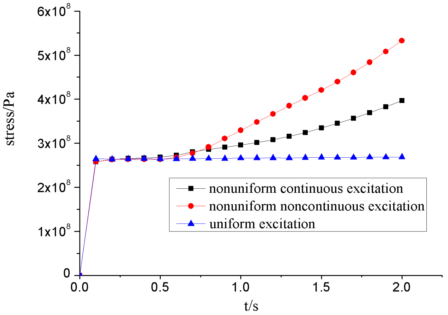
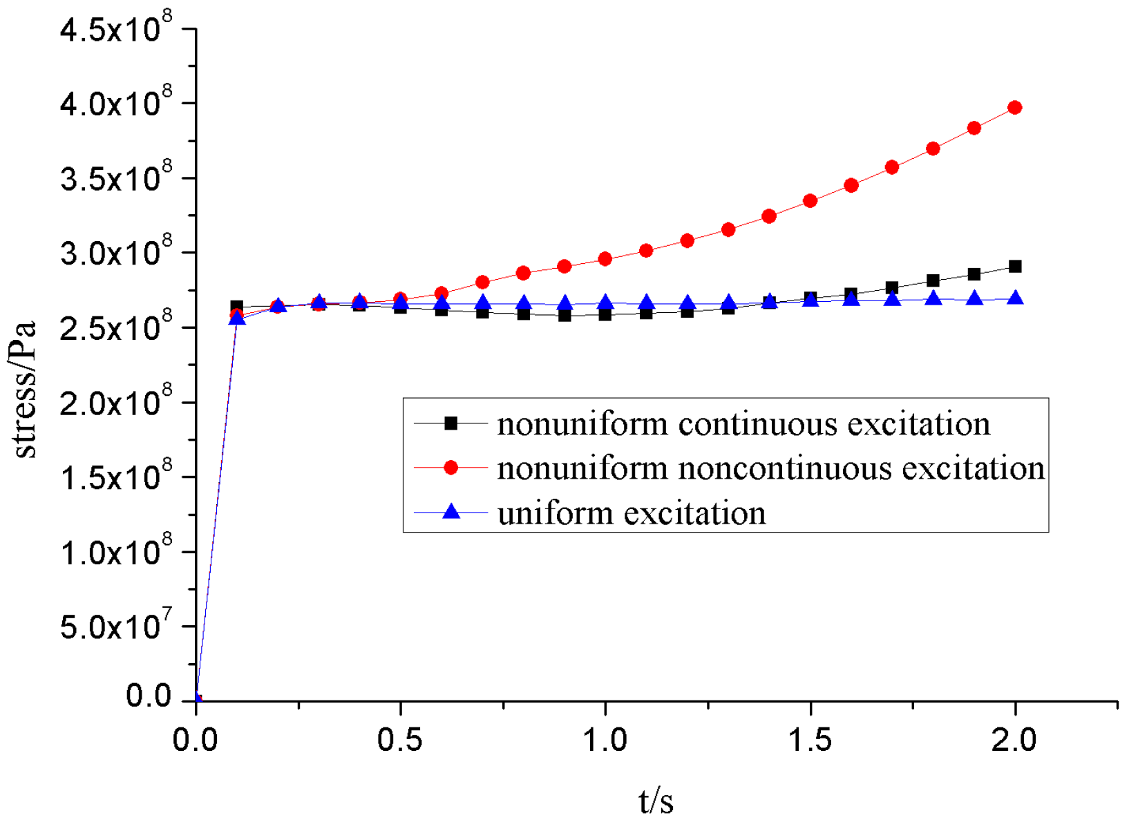
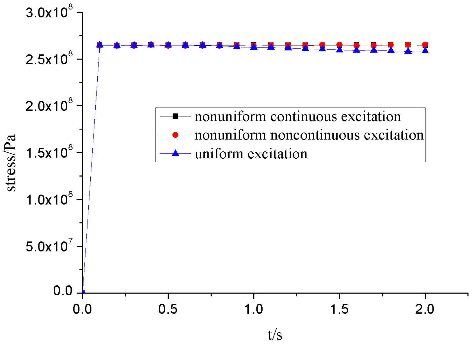
Through the finite element simulation of three kinds of working conditions, the stress at the maximum, middle, and end of the pipeline stress can be compared, as shown in Figure 4, Figure 5 and Figure 6, respectively.

As mentioned above, when analyzing the maximum stress value and middle stress value of the pipeline, the nonuniform excitation stress value is larger than the uniform excitation stress value, which indicates that it is necessary to take into account the influence of spatial variation on the earthquake response of long-distance pipeline. The stress value of nonuniform noncontinuous configuration is larger than the nonuniform stimulus, which further reflects the spatial effect. However, at the end of the pipeline, the stress values for the three conditions are not substantially different. These results show that if the pipeline is a “point” structure, there is no spatial influence of the loads.

7. Fuzzy Damage Analysis of the Pipeline

7.1. Fuzzy Damage Model

The structure has three states to assess the safety: the failure state, the limit state and the safety state. The structural transition from safety to failure occurs in a sudden manner. However, if the stress value exceeds the specific stress value, it does not mean that the structure is completely reliable. When the value of function is less than specific stress value, the structure is not completely destroyed. The degree of structural damage is an adaptive process that involves a vague range between reliability and failure, as shown in Figure 7. Thus, this paper proposes a fuzzy reliability evaluation model that is suitable for the pipeline integrity based on the theory of fuzzy mathematics.

When it is defined that the structure in a definite state as a fuzzy event $\tilde{B}$, the fuzzy event $\tilde{B}$ is represented by the membership function of state variable $\tilde{Z}$ to $\tilde{B}$:

$${\tilde{u}}_B(z)=\{\begin{array}{l}1\\ F(z),F(z)\in (0,1)\\ 0\end{array}$$

(37)

The practical seismic damage has no clear classification, so it is a fuzzy concept, and the damage degree of each component of the pipeline is different. In addition, the results of the damage assessment of pipelines by different methods are not the same. Therefore, based on the three states of failure criteria for the pipeline [33,34], the division of the degree of damage is shown in

Table 7. Division of the degree of damage to pipelines.

Earthquake Damage Level	Description	Quantitative Indicators
Essentially intact	The pipe may be slightly deformed, but it is not damaged, there is no leakage, and it can continue to operate without repair.	$\sigma <0.8{\sigma }_{\mathrm{s}}$
Medium damage	Large deformation or buckling of the pipeline, slight damage, leakage, affecting the gas supply but allowing resumption of operation after emergency repair.	$0.8{\sigma }_{\mathrm{s}}<\sigma <0.8{\sigma }_{\mathrm{b}}$
Severe damage	The pipe is broken, and the interface is pulled off, causing secondary disasters and requiring replacement.	${\sigma }_{\mathrm{b}}<\sigma$

. According to fuzzy mathematics, this paper establishes a fuzzy damage model of pipeline to assess the seismic risk.

The fragility domains of the pipeline are defined as follows:

$U$ = [basic intact, minor damage, medium damage; severe damage; destruction]

Hence, this parameter can be expressed as

$$U=\left[A_1,A_2,A_3,A_4,A_5\right]$$

(38)

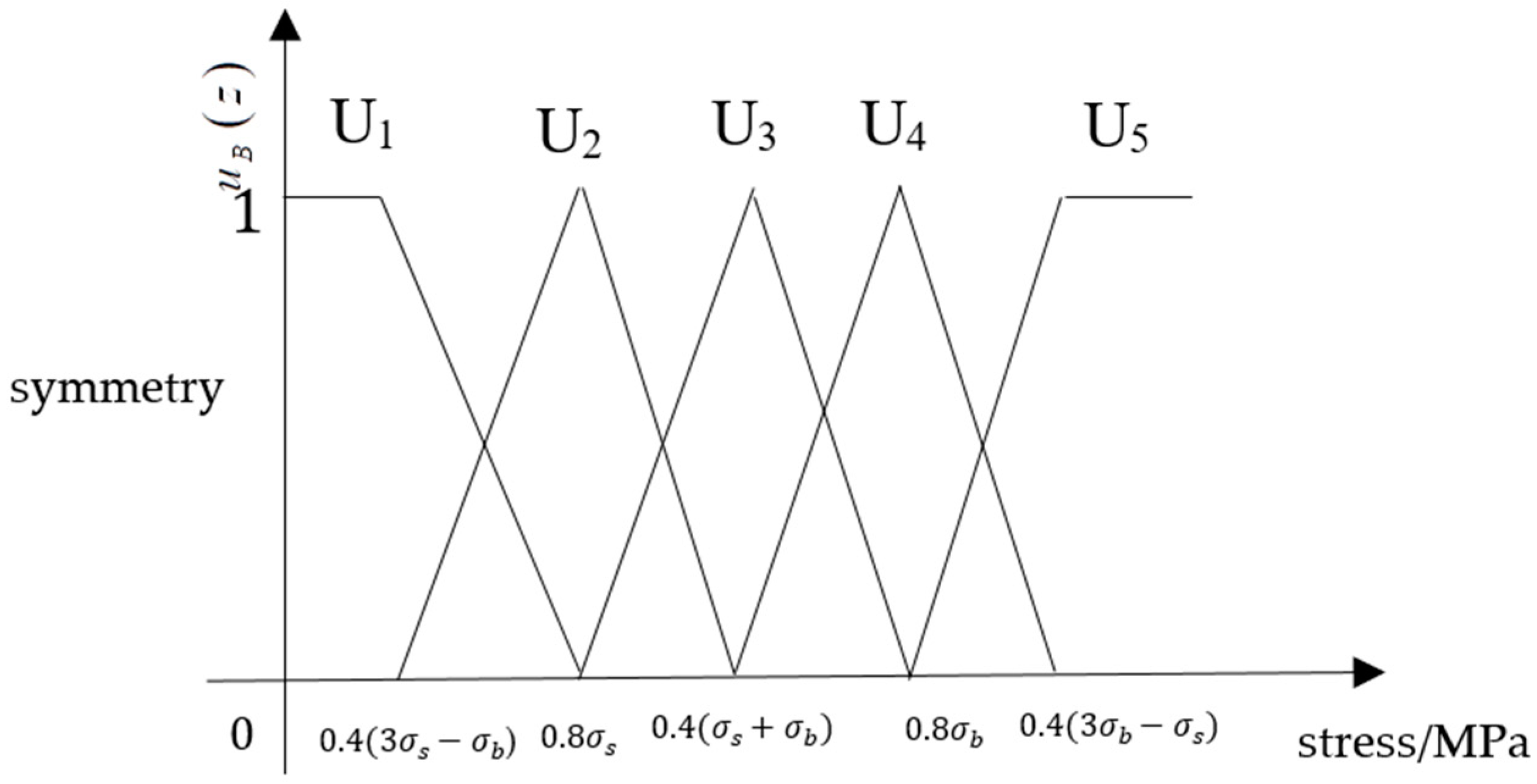
As with fuzzy mathematical theory, the fuzzy subset can be described as $A_i(i=1,2,3,4,5)\in \left[0,1\right]$. As shown in Figure 8, we can establish membership functions to express the distribution of $A_i$ as follows:

$${\mu }_{{\tilde{B}}_1(z)=}\{\begin{array}{c}1,0\le z\le 0.4(3{\sigma }_{\mathrm{s}}-{\sigma }_{\mathrm{b}})\\ =\frac{2.5}{{\sigma }_{\mathrm{s}}-{\sigma }_{\mathrm{b}}}z+\frac{2{\sigma }_{\mathrm{s}}}{{\sigma }_{\mathrm{b}}-{\sigma }_{\mathrm{s}}},0.4(3{\sigma }_{\mathrm{s}}-{\sigma }_{\mathrm{b}})\le z\le 0.8{\sigma }_{\mathrm{s}}\end{array}$$

(39)

$${\mu }_{{\tilde{B}}_2(z)=}\{\begin{array}{c}\frac{-2.5}{{\sigma }_{\mathrm{s}}+{\sigma }_{\mathrm{b}}}z+\frac{3{\sigma }_{\mathrm{s}}+{\sigma }_{\mathrm{b}}}{{\sigma }_{\mathrm{s}}+{\sigma }_{\mathrm{b}}},0.4(3{\sigma }_{\mathrm{s}}-{\sigma }_{\mathrm{b}})\le z\le 0.8{\sigma }_{\mathrm{s}}\\ \frac{2.5}{{\sigma }_{\mathrm{s}}-{\sigma }_{\mathrm{b}}}z+\frac{3{\sigma }_{\mathrm{s}}+{\sigma }_{\mathrm{b}}}{{\sigma }_{\mathrm{b}}-{\sigma }_{\mathrm{s}}},0.8{\sigma }_{\mathrm{s}}\le z\le 0.4({\sigma }_{\mathrm{s}}+{\sigma }_{\mathrm{b}})\end{array}$$

(40)

$${\mu }_{{\tilde{B}}_3(z)=}\{\begin{array}{c}\frac{2.5}{{\sigma }_{\mathrm{b}}-{\sigma }_{\mathrm{s}}}z+\frac{2{\sigma }_{\mathrm{s}}}{{\sigma }_{\mathrm{s}}-{\sigma }_{\mathrm{b}}},0.8{\sigma }_{\mathrm{s}}\le z\le 0.4({\sigma }_{\mathrm{s}}+{\sigma }_{\mathrm{b}})\\ \frac{2.5}{{\sigma }_{\mathrm{s}}-{\sigma }_{\mathrm{b}}}z+\frac{2{\sigma }_{\mathrm{b}}}{{\sigma }_{\mathrm{b}}-{\sigma }_{\mathrm{s}}},0.4({\sigma }_{\mathrm{s}}+{\sigma }_{\mathrm{b}})\le z\le 0.8{\sigma }_{\mathrm{b}}\end{array}$$

(41)

$${\mu }_{{\tilde{B}}_4(z)=}\{\begin{array}{c}\frac{2.5}{{\sigma }_{\mathrm{b}}-{\sigma }_{\mathrm{s}}}z+\frac{{\sigma }_{\mathrm{s}}+{\sigma }_{\mathrm{b}}}{{\sigma }_{\mathrm{s}}-{\sigma }_{\mathrm{b}}},0.4({\sigma }_{\mathrm{s}}+{\sigma }_{\mathrm{b}})\le z\le 0.8{\sigma }_{\mathrm{b}}\\ \frac{2.5}{{\sigma }_{\mathrm{s}}-{\sigma }_{\mathrm{b}}}z+\frac{{\sigma }_{\mathrm{s}}-3{\sigma }_{\mathrm{b}}}{{\sigma }_{\mathrm{s}}-{\sigma }_{\mathrm{b}}},0.8{\sigma }_{\mathrm{b}}\le z\le 0.4(3{\sigma }_{\mathrm{b}}-{\sigma }_{\mathrm{s}})\end{array}$$

(42)

$${\mu }_{{\tilde{B}}_5(Z)=}\{\begin{array}{c}\frac{2.5}{{\sigma }_{\mathrm{b}}-{\sigma }_{\mathrm{s}}}z+\frac{2{\sigma }_{\mathrm{b}}}{{\sigma }_{\mathrm{s}}-{\sigma }_{\mathrm{b}}},0.8{\sigma }_{\mathrm{b}}\le z\le 0.4(3{\sigma }_{\mathrm{b}}-{\sigma }_{\mathrm{s}})\\ 1,0.4(3{\sigma }_{\mathrm{b}}-{\sigma }_{\mathrm{s}})\le z\end{array}$$

(43)

where $\delta (A,B)$ is the value of Euclidean closeness; $a_i$ is the corresponding element of the vulnerability fuzzy subset; and $b_i$ is the corresponding elements of the standard vulnerability fuzzy subset.

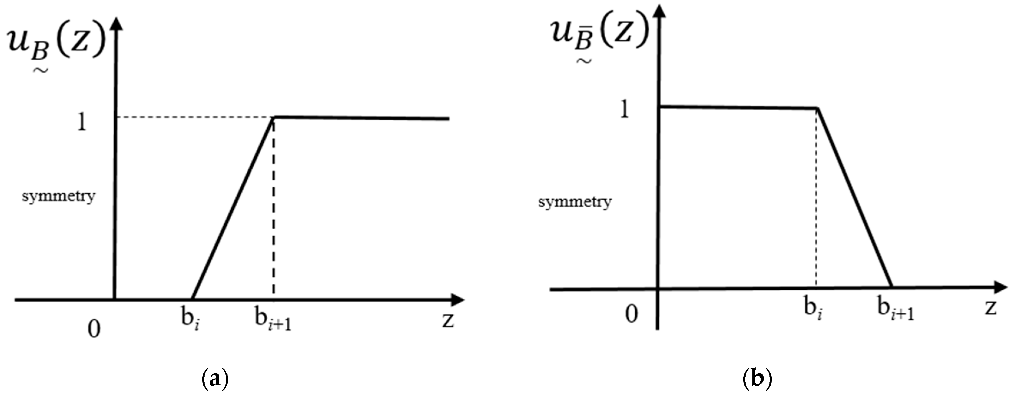
From the fuzzy region of the earthquake damage level $\underset{~}{B}$, the paper establishes a fuzzy region of structural response $\underset{~}{B}$ with a higher level of seismic damage than $\underset{~}{B}$, as shown in Figure 9a. Therefore, we can also obtain the fuzzy safe field of $\overline{\underset{~}{B}}$ based on the fuzzy mathematical theory, as shown in Figure 9b, while their membership function can be expressed as

$$u_{\overline{\underset{~}{B_i}}}(z)+u_{\underset{~}{B_i}}(z)=1$$

(44)

Clearly, when the structure’s response is in a fuzzy safety field, the structure does not break. Considering that the seismic response is ambiguous, the structural response also has random characteristics. The structural safety guidelines can be expressed as

$$\chi =\left\{-\overline{\underset{~}{B}}\underset{~}{\supset }X(\sigma ,t)\underset{~}{\subset }\overline{\underset{~}{B}},\forall t\in T\right\}$$

(45)

where $X(\sigma ,t)$ is the structural reaction and $T$ is the duration time of the earthquake.

Combined with Section 6, this paper proposes a fuzzy description to define the degree of structural damage. Thus, using the fuzzy membership function model can evaluate the damage state of the structure. Therefore, the fuzzy set of the structure can be defined as

$$\underset{~}{B}=\frac{\underset{~}{B(x_1)}}{U_1}+\frac{\underset{~}{B(x_2)}}{U_2}+\frac{\underset{~}{B(x_3)}}{U_3}+\frac{\underset{~}{B(x_4)}}{U_4}+\frac{\underset{~}{B(x_5)}}{U_5}$$

(46)

7.2. Application of Pipeline Analysis

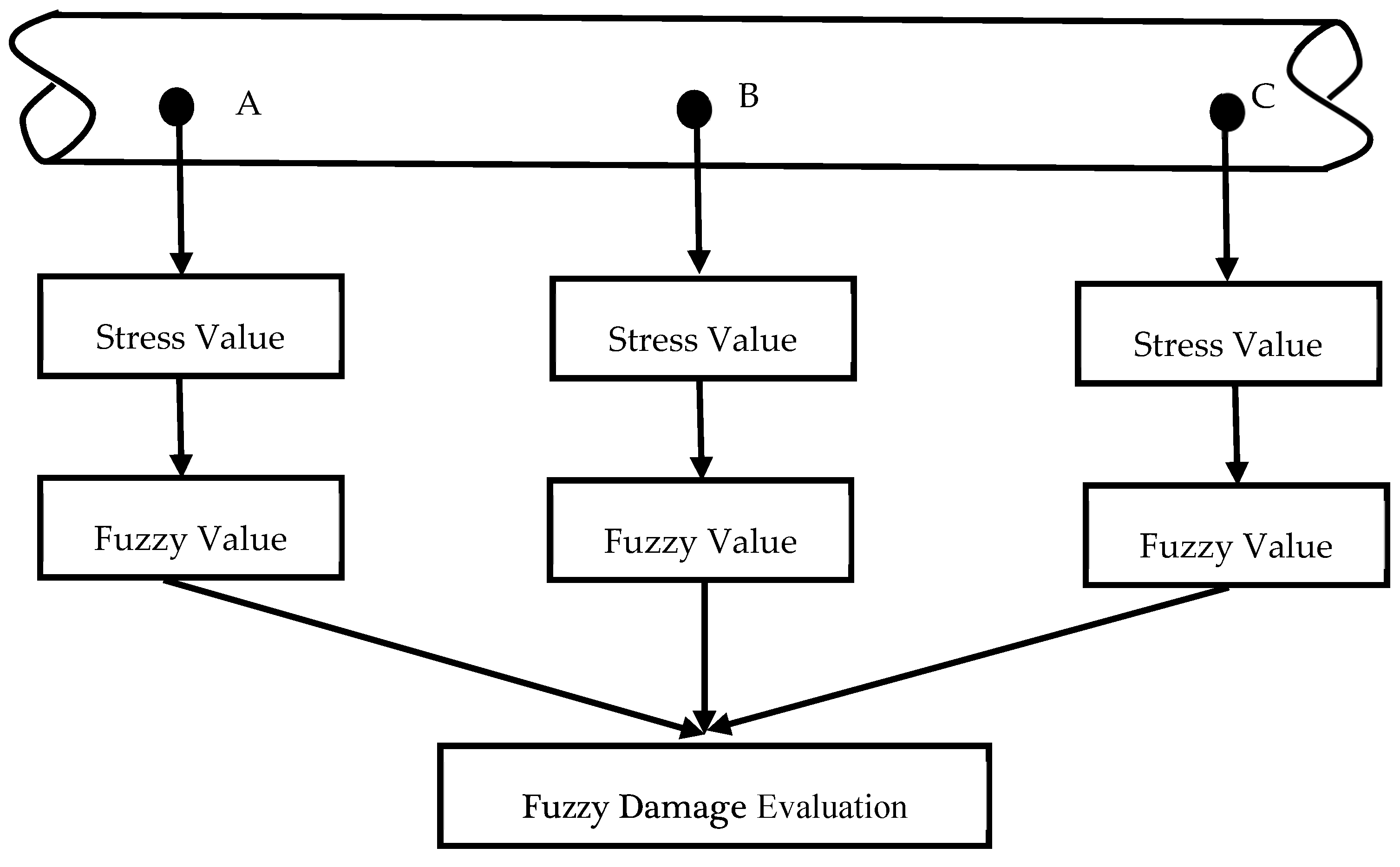
Safety evaluations generally refer to the stress-based failure principle and strain-based failure principle. Those methods all cause results divided into two completely opposite states: “good” and “failed”. Actually, the system is in an intact state or the failure state is ambiguous at any moment. Therefore, a fuzzy damage criterion is proposed to evaluate the statue of the pipeline, which links the value of stress and fuzzy value. Figure 10 shows an example of a process from three varying points (A, B and C) along the pipeline. Under this situation, the process can realize fuzzification of values and perform fuzzy evaluation. Since there are a large amount of data to show the change of damage for pipeline, we can construct the system of the degree of damage.

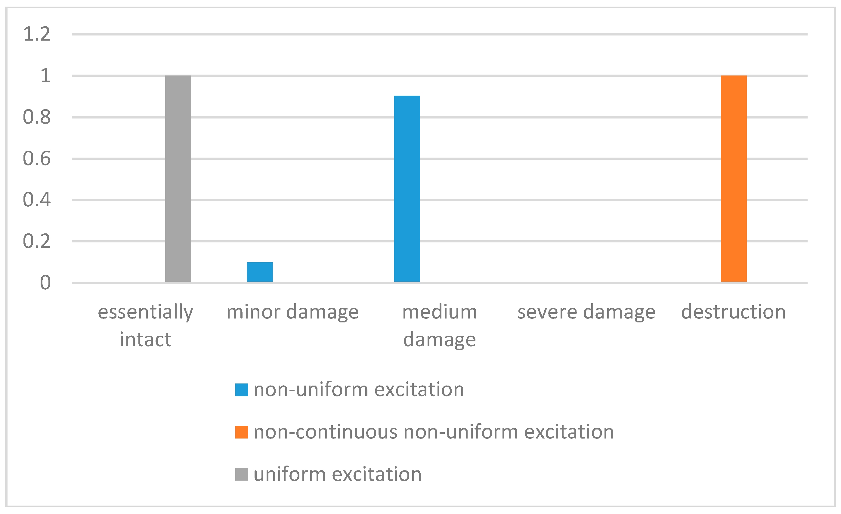
According to the results of Section 6, this paper analyzes the degree of fuzzy damage when the pipeline is exposed to a random seismic load. The case is taken into the most representative value for the stress value of the pipeline. When selecting the maximum stress value for time-varying analysis, we obtain the following equation to define the damage level of the structural integrity:

$$\underset{~}{a}=\frac{1}{U_1}+\frac{0}{U_2}+\frac{0}{U_3}+\frac{0}{U_4}+\frac{0}{U_5}$$

(47)

$$\underset{~}{b}=\frac{0}{U_1}+\frac{0.098}{U_2}+\frac{0.902}{U_3}+\frac{0}{U_4}+\frac{0}{U_5}$$

(48)

$$\underset{~}{c}=\frac{0}{U_1}+\frac{0}{U_2}+\frac{0}{U_3}+\frac{0}{U_4}+\frac{1}{U_5}$$

(49)

Clearly, as shown in Figure 11, using the fuzzy seismic damage model established in this paper not only evaluates the degree of structural damage very intuitively but also constructs a fuzzy safety criterion for the structure. This approach also verifies the importance of random space-time loads in seismic analysis. Using fuzzy damage levels, structural safety guidelines can describe the failure of a structure that does not occur at a certain level or higher level based on structural responses.

8. Conclusions

Based on the theory of random process and random field, this paper proposes the concept of a random space-time seismic load through coupling multiple factors. After considering the site conditions and the nonstationary nature of the load, a nonstationary spectral density function with space-time characteristics suitable for a long-distance pipeline is established. In addition, a reasonable assessment model for the pipeline is proposed to degree of damage based on fuzzy mathematics. A combined analysis with numerical simulation and fuzzy damage criteria gives the following conclusions:

• Using random processes and random fields, the coupling of a universal stochastic space-time earthquake load based on the power spectrum is investigated, and the seismic load of space-time characteristics is summarized.
• For long-distance pipelines, under the action of earthquake loads, it is necessary to consider not only the time-varying characteristics with time but also the factors brought about by the spatial characteristics. Due to the influence of spatial factors on the long-distance pipeline, relative to non-uniform excitation, the result will be quite different.
• The response of a long-distance pipeline under nonuniform earthquake excitation is solved, and it is of great significance to establish the response design system for a long-distance pipeline under an earthquake.
• Establishing the fuzzy damage model of the pipeline and the fuzzy safety criterion can more reasonably describe the damage of the structure with a certain level or higher level. This approach has laid the foundation for the establishment of comprehensive assessment of pipeline safety in the future.

References

1. Wen, K.; He, L.; Yu, W.; Gong, J. A Reliability Assessment of the Hydrostatic Test of Pipeline with 0.8 Design Factor in the West-East China Natural Gas Pipeline III. Energies 2018, 11, 1197. [Google Scholar] [CrossRef]
2. He, B.J.; Zhao, D.X.; Zhu, J.; Darko, A.; Gou, Z.H. Promoting and implementing urban sustainability in China: An integration of sustainable initiatives at different urban scales. Habitat Int. 2018, 82, 83–93. [Google Scholar] [CrossRef]
3. Mou, B.; He, B.J.; Zhao, D.X.; Chau, K.W. Numerical simulation of the effects of building dimensional variation on wind pressure distribution. Eng. Appl. Comput. Fluid 2017, 11, 293–309. [Google Scholar] [CrossRef] [Green Version]
4. Zhang, Z.C.; Lin, J.H.; Zhang, Y.H.; Zhao, Y.; Howson, W.P.; Williams, F.W. Non-stationary random vibration analysis for train–bridge systems subjected to horizontal earthquakes. Eng. Struct. 2010, 32, 3571–3582. [Google Scholar] [CrossRef]
5. CEM. Eurocode 8: Design of Structure for Earthquake Resistance-Part 2: Bridges: European Standard EN 1998-2: 2005; Comite European de Normalisation: Brusells, Belgium, 2005. [Google Scholar]
6. Hindy, A.; Novak, M. Pipeline response to stochastic ground motion. J. Eng. Mech. Div. 1980, 106, 339–360. [Google Scholar]
7. Loh, C.H. Analysis of the spatial variation of earthquake waves and ground movements from smart-1 array data. Earthq. Eng. Struct. Dyn. 2010, 13, 561–581. [Google Scholar] [CrossRef]
8. Wan, Y. Orthogonal Expansion-Stochastic Function Model of Engineering Stochastic Excitation and Its Application; Three Gorges University: Yi Chang, China, 2014. [Google Scholar]
9. Li, J.; Liu, Z.J. Stochastic process expansion method based on standard orthogonal basis. J. Tongji Univ. (Nat. Sci. Ed.) 2006, 3410, 1279–1283. [Google Scholar] [CrossRef]
10. Liu, Z.J.; Li, J. Orthogonal expansion of stochastic processes of ground motion. J. Tongji Univ. (Nat. Sci. Ed.) 2008, 36, 1153–1159. [Google Scholar] [CrossRef]
11. He, X.; Zhao, H.; Cai, W.; Liu, Z.; Si, S.Z. Earthquake networks based on space–time influence domain. Phys. A Stat. Mech. Appl. 2014, 407, 175–184. [Google Scholar] [CrossRef]
12. Zadeh, L.A. Fuzzy sets. Inf. Control 1965, 8, 338–353. [Google Scholar] [CrossRef] [Green Version]
13. Jamshidi, A.; Yazdani-Chamzini, A.; Yakhchali, S.H.; Khaleghi, S. Developing a new fuzzy inference system for pipeline risk assessment. J. Loss Prev. Process. Ind. 2013, 26, 197–208. [Google Scholar] [CrossRef]
14. Markowski, A.S.; Mannan, M.S. Fuzzy logic for piping risk assessment (pflopa). J. Loss Prev. Process. Ind. 2009, 22, 921–927. [Google Scholar] [CrossRef]
15. Lazarian, A.; Vishniac, E.T. Reconnection in a weakly stochastic field. Astrophys. J. 2012, 517, 700–718. [Google Scholar] [CrossRef]
16. Ye, J.H.; Zhang, Z.Q.; Chu, Y. Strength behavior and collapse of spatial-reticulated structures under multi-support excitation. Sci. China Technol. Sci. 2011, 54, 1624–1638. [Google Scholar] [CrossRef]
17. Ye, J.; Pan, J.; Liu, X. Vertical coherency function model of spatial ground motion. Earthq. Eng. Eng. Vib. (Engl. Vers.) 2011, 10, 403. [Google Scholar] [CrossRef]
18. Bi, K.; Hao, H. Influence of irregular topography and random soil properties on coherency loss of spatial seismic ground motions. Earthq. Eng. Struct. Dyn. 2011, 40, 1045–1061. [Google Scholar] [CrossRef]
19. Shinozuka, M.; Saxena, V.; Deodatis, G. Effect of spatial variation of ground motion on highway structures. Caries Res. 2000, 42, 79–87. [Google Scholar] [CrossRef]
20. Luco, J.; Wong, H. Response of a rigid foundation to a spatially stochastic ground motion. Earthq. Eng. Struct. Dyn. 1986, 14, 891–908. [Google Scholar] [CrossRef]
21. Wiener, N. Generalized harmonic analysis. Acta Math. 1930, 55, 117–258. [Google Scholar] [CrossRef]
22. Clough, R.W.; Penzien, J. Dynamics of Structures; McGraw-Hill: New York, NY, USA, 1993. [Google Scholar]
23. Ma, X.; Vakakis, A.F.; Bergman, L.A. Karhunen–Loeve analysis and order reduction of the transient dynamics of linear coupled oscillators with strongly nonlinear end attachments. J. Sound Vib. 2008, 309, 569–587. [Google Scholar] [CrossRef]
24. Seya, H.; Talbott, M.E.; Hwang, H.H.M. Probabilistic earthquake analysis of a steel frame structure. Probab. Eng. Mech. 1993, 8, 127–136. [Google Scholar] [CrossRef]
25. Dumanogluid, A.A.; Soyluk, K. A stochastic analysis of long span structures subjected to spatially varying ground motions including the site-response effect. Eng. Struct. 2003, 25, 1301–1310. [Google Scholar] [CrossRef]
26. Yan, S.H.; Liang, B.; Gao, F. Dynamic reliability analysis of resistance of tunnels longitudinal non-stationarity earthquake. J. Rock Mech. Eng. 2005, 24, 818–822. [Google Scholar] [CrossRef]
27. Cao, Z.; Xue, S.D.; Wang, X.S.; Liu, Y.C. Selection of earthquake waves and values of damping ratio for space structures in aseismic analysis. Spat. Struct. 2008, 14, 3–8. [Google Scholar] [CrossRef]
28. Davenport, A.G. Note on the distribution of the largest value of a random function with application to gust loading. Proc. Inst. Civ. Eng. 1964, 28, 187–196. [Google Scholar] [CrossRef]
29. Lin, J.; Li, J.; Zhang, W.; Williams, F.W. Non-stationary stochastic earthquake responses of multi-support structures in evolutionary inhomogeneous stochastic fields. Earthq. Eng. Struct. Dyn. 1997, 26, 135–145. [Google Scholar] [CrossRef]
30. Bubenik, T.A.; Olson, R.J.; Stephens, D.R.; Francini, R.B. Analyzing the Pressure Strength of Corroded Line Pipe; Offshore Mechanics and Arctic Engineering: Calgary, AB, Canada, 1992. [Google Scholar]
31. Flügge, W. Handbook of Engineering Mechanics; McGraw-Hill: New York, NY, USA, 1962. [Google Scholar]
32. Ye, L.P.; Lu, X.Z. Analysis on seismic damage of building in the Wenchuan earthquake. J. Archit. Struct. 2008, 29, 1–9. [Google Scholar] [CrossRef]
33. Rimkevicius, S.; Kaliatka, A.; Valincius, M.; Dundulis, G.; Janulionis, R.; Grybenas, A.; Zutautaite, I. Development of approach for reliability assessment of pipeline network systems. Appl. Energy 2012, 94, 22–33. [Google Scholar] [CrossRef]
34. Urban Construction Research Institute. CJJ/T 81-2013 Technical Specification for Directly Buried Hot Water Pipeline for Urban Heating; China Building Industry Press: Beijing, China, 2013. [Google Scholar]
Figure 1. Function of self-power spectral density.
Energies 12 00062 g001
Figure 2. Pressure pipeline model.
Energies 12 00062 g002
Figure 3. Division of the grid.
Energies 12 00062 g003
Figure 4. Comparison of the maximum stress point of the pipeline.
Energies 12 00062 g004
Figure 5. Comparison of stress at the middle of the pipeline.
Energies 12 00062 g005
Figure 6. Comparison of stress at the end of the pipeline.
Energies 12 00062 g006
Figure 7. Fuzzy damage state of the structure.
Energies 12 00062 g007
Figure 8. Function of different fragility levels.
Energies 12 00062 g008
Figure 9. Membership function of the fuzzy damage field. (a) Fuzzy fail field; (b) Fuzzy safe field.
Energies 12 00062 g009
Figure 10. Estimation of logic for damage fuzzy evaluation in the pipeline.
Energies 12 00062 g010
Figure 11. Fuzzy damage of three working conditions.
Energies 12 00062 g011