A Cluster-Based Baseline Load Calculation Approach for Individual Industrial and Commercial Customer
by
Tianli Song
1,2,*, 
Yang Li
1,
Xiao-Ping Zhang
2,
Jianing Li
2,
Cong Wu
2,
Qike Wu
3 and
Beibei Wang
1 1
School of Electrical Engineering, Southeast University, Nanjing 210096, China
2
Department of Electronic, Electrical and Systems Engineering, University of Birmingham, Birmingham B15 2TT, UK
3
Guangzhou Power Supply Bureau Limited Company, Guangzhou 510620, China
*
Author to whom correspondence should be addressed.
Energies 2019, 12(1), 64; https://doi.org/10.3390/en12010064
Submission received: 29 October 2018
/
Revised: 15 December 2018
/
Accepted: 21 December 2018
/
Published: 26 December 2018
(This article belongs to the Special Issue Demand Response in Electricity Markets)
Abstract
:Demand response (DR) in the wholesale electricity market provides an economical and efficient way for customers to participate in the trade during the DR event period. There are various methods to measure the performance of a DR program, among which customer baseline load (CBL) is the most important method in this regard. It provides a prediction of counterfactual consumption levels that customer load would have been without a DR program. Actually, it is an expected load profile. Since the calculation of CBL should be fair and simple, the typical methods that are based on the average model and regression model are the two widely used methods. In this paper, a cluster-based approach is proposed considering the multiple power usage patterns of an individual customer throughout the year. It divides loads of a customer into different types of power usage patterns and it implicitly incorporates the impact of weather and holiday into the CBL calculation. As a result, different baseline calculation approaches could be applied to each customer according to the type of his power usage patterns. Finally, several case studies are conducted on the actual utility meter data, through which the effectiveness of the proposed CBL calculation approach is verified.
1. Introduction
In most modern power systems, the problems of periodic and structural power shortage and sharper peak-valley difference exist for a long time. These raise concerns over resource depletion and bridging the gap between power supply and demand. However, with the increased participation of demand side resources in electricity market, demand response (DR) has been widely known as an important means to balance supply and demand [1,2,3]. DR appeals customers to temporarily reduce, shift, or shed their demand in response to price signals or other market incentives during the event period [4]. To this end, quantifying the demand reduction is becoming a major issue for both electrical unities and customers.
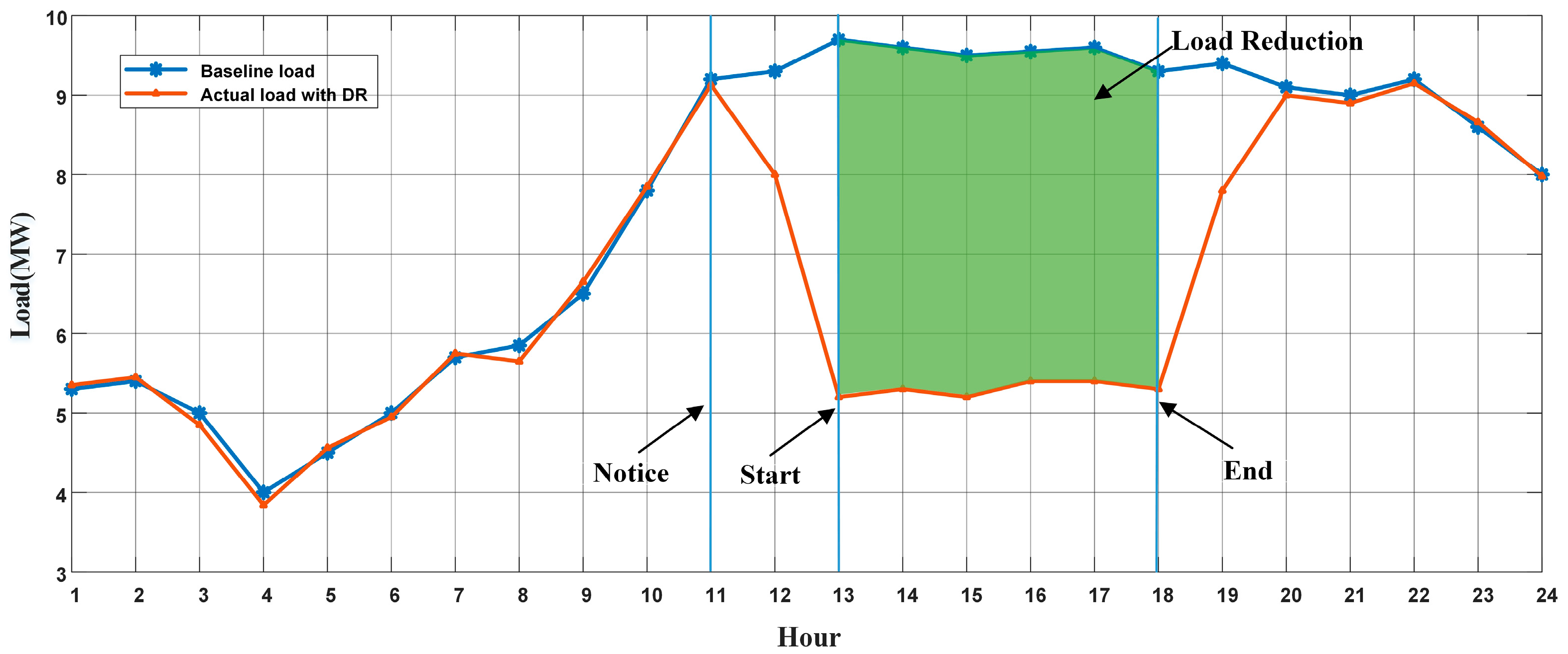
Transparent rights and simple rules are significant for DR program implementation [5]. Demand subscription service is an approach that provides a two-sided contract. In order to ensure the benefits of both sides in DR programs, it is necessary to calculate customer baseline load (CBL). CBL attempts to predict what customer load would have been under ‘normal’ (non-DR event) circumstances, so that the amount of customer load reduction could be obtained [6,7]. Figure 1 explicitly illustrates what CBL is during a typical DR event.
A properly designed baseline methodology is perhaps the most important determinant of the success of any DR program—it enables grid operators and utilities to measure the performance of DR resources [8]. The methods of calculating CBL are required to be simple, transparent, and easy to understand for both utilities and customers. Usually, there are three steps to calculate CBL: (1) data selection, (2) calculation, and (3) adjustment.
The data selection determines which data are chosen for the calculation of CBL. If the DR event day is a working day (holiday), then the chosen data of proceeding days should be working days (holidays). The calculation means that what kind of methodology is used to predict CBL. The existing CBL calculation methods that are based on the average model and regression model are the two widely used methods of the different independent system operators (ISO) in the USA [9,10]. With regards to the adjustment, it is to calculate the impact of other factors like ‘weather’ in special circumstances. The initial baseline can be adjusted upward/downward according to the load or weather condition of several hours before/during the DR event period.
Based on the calculation process that is mentioned above, when there is a further requirement for the accuracy of CBL calculation, a data mining method based on artificial neural network and clustering appears [6,11,12]. By analyzing the electrical characteristics of customers, the different kinds of methods for calculating CBL can be applied according to the different types of customers, but this study assumes that each customer would have only one power usage pattern throughout the year. The study of the University of California, Berkeley showed that the evidence from field studies quantify the difference in evaluation results between randomized controlled trial (RTC) methods and quasi-experimental methods [13]. RTCs are widely viewed as the ‘gold standard’ of evaluation, but it needs a rich set of field experiments. In addition, there are also some studies that analyzed the accuracy and bias of CBL [14,15].
The objective of this paper is to present a cluster-based CBL method that considers the multiple power usage patterns of a customer throughout the year. Unlike the common methods, which calculate CBL with fixed authorism and steps, the proposed approach brings in the concept of considering the multiple load consumption patterns of each customer. It first clusters loads of a customer based on his power usage patterns. Within each cluster, the power usage patterns of a customer are further divided into different types based on the weather or holiday sensitive status. Subsequently, each customer could have one or two CBL calculation methods according to the type of his power usage patterns throughout the year. In addition, for the customers with weather or holiday sensitive power usage patterns, we need to consider the holiday data and the weather adjustment. By contrast, for the customers with neither holiday nor weather sensitive power usage patterns, we could omit the process of selecting designated data and calculating adjustment. Therefore, it can be much easier and transparent to calculate CBL for both utilities and customers.
2. The General Framework of Calculating CBL
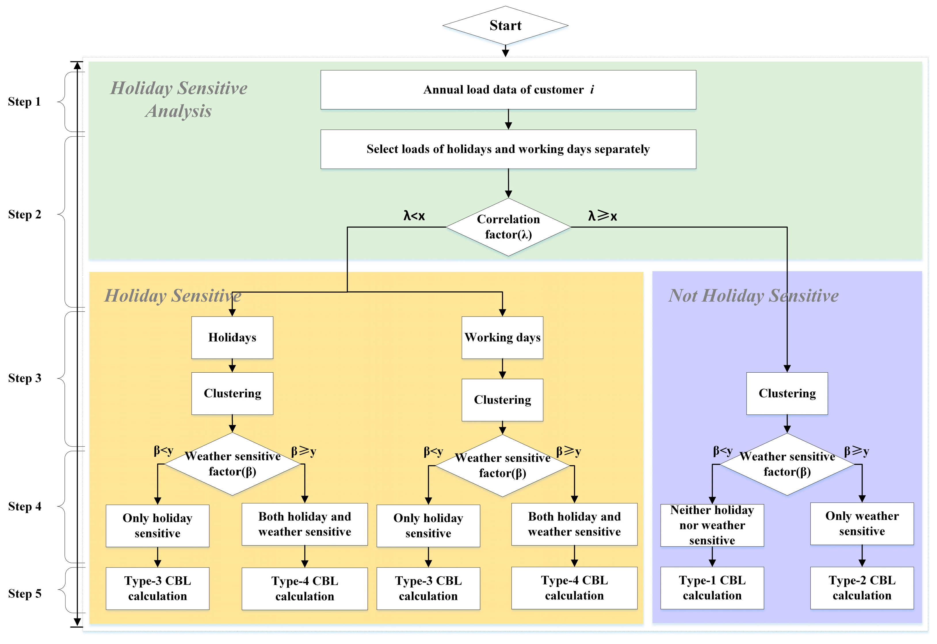
In this paper, a CBL calculation method is proposed basing on data-mining techniques with an unsupervised learning, as shown in Figure 2. The whole calculation process contains five steps.
1. Data preprocessing
Data preprocessing includes data selection and cleaning. The data selection means that the selected data are the daily 24-hour load data of an industrial and commercial customer throughout the year in an area. The data cleaning includes discontinuous data completion and abnormal data correction. Unlike the general studies [7,12], since the data used in clustering are loads of each customer instead of a group of customers, we do not need normalization here.
2. Holiday sensitive analysis.
We choose each individual customer’s loads of working days and holidays separately, then analyzing the coincidence degree of the two types of days. If the coincidence degree (λ) is more than (x), then the loads of working days and holidays are considered in high similarity, so they can be put together. If not, we need to put them separately.
3. Clustering analysis.
We use a quadratic clustering method to classify the individual customer’s loads: the first clustering uses the system clustering method and the second clustering uses the fuzzy C-means method.
4. Weather sensitive analysis.
The average load of a day and the maximum temperature are used to make the linear regression analysis. If the correlation factor is over (y), then this kind of loads will be seen as weather sensitive, so we need to calculate the CBL of them with weather adjustment method. If not, we can just use a simple method without adjustment.
5. CBL calculation.
Based on the work above, in order to find a preferable method for each type of power usage pattern, three different calculation and adjustment methods are tested to calculate CBL. It is noticed that each customer may have one or two types of power usage patterns throughout the year.
Upon completion of step 5 for the customer (i), the next customer (i+1) will be selected for a new round of CBL calculation. By analyzing each customer’s historical load data, we will give a suitable CBL calculation method for each type.
3. Baseline Estimation Methods for Individual Customer
3.1. Data-Mining Approach Based on Clustering Analysis
The data-mining model for CBL calculation is based on clustering. Clustering is a useful tool for data analysis and it has been widely used in the study of the modern power system, such as electrical consumption analysis [7] and electrical load prediction [16,17]. Various clustering algorithms have been studied in previous work, including hierarchical clustering, affinity propagation clustering, and fuzzy c-means clustering.
In this paper, due to the large data of samples (24 points daily load data throughout the year) and the load characteristic indexes that we used in the clustering, it may be not accurate if we only use one clustering method. So, in order to effectively recognize the load samples, we need to use a clustering method that fits the large numbers calculation. It is observed that the setting of the initial clustering center has great influence on the clustering effect of the fuzzy C-means method, which leads to the instability of the results. By contrast, the system clustering method is repetitive when processing large samples, but its process is simple and intuitive, and the classification is fast and does not require the initial set of classical clustering algorithms. Therefore, we use the quadratic clustering method to classify the user load characteristics. The first clustering uses the system clustering method and the second clustering uses the fuzzy C-means method. The centers of the second cluster are provided by the first system clustering results. As a result, it not only avoids the problem that the fuzzy c-means clustering is sensitive to the initial dataset, but it also achieves the classification accuracy.
Since the data-mining algorithm is the basis of the whole work in this paper, we still need to analyze the correlation between electrical load and temperature [18,19]. Therefore, after obtaining the clustering centers, it is also necessary to further consider the load characteristics index, such as load rate and peak-valley difference rate. By optimizing the quadratic clustering results, the clustering centers with load rate and peak-valley difference rate are combined together to make the results more representative, and the different characteristics between different load data can be more clearly distinguished. As a result, correlation analysis between load and temperature will become more reasonable and effective.
3.2. CBL Calculation Methods
Once the annual loads of a customer are clustered into different power usage patterns, the next is to calculate CBL on event days within each pattern. The calculation of CBL requires being fair and simple. The simplest method is to use the average loads of previous days. It is worth noting that some of these methods are similar to the methods in short-term load forecasting, which predicts the overall load profiles of a group of users. However, for CBL prediction, we need to calculate CBL for each individual customer. Since each customer’s load is much more uncertain, the prediction could be more difficult.
3.2.1. Simple Average Model-High X of Y
We firstly select the X highest “average daily kWh usage” days from a pool of Y days before DR day. Subsequently, for each hour of the day, power consumption of X selected days will be averaged, and this average value will represent CBL.
where is the actual customer load before the DR event day on day at timeslot ; is the calculated value of CBL for customer i.
3.2.2. Simple Average Model-Middle X of Y
We still choose X days from a pool of Y days before the DR event day, but it is worth noticing that we will eliminate the highest and the lowest “average daily kWh usage” days, and then the load of rest days will be averaged.
where is the actual customer load before the DR event day on day at timeslot t; is the calculated value of CBL for customer i.
3.2.3. Exponential Smoothing Model
Exponential Smoothing is sequence analysis method, it weights past observations with exponentially decreasing weights to forecast a future. The first step is the same as method ‘High X of Y’, and the equation (3) is showing weighted recent data for a new CBL prediction.
where is the estimation value of the new baseline, is the actual electric demand at a time on day. uses an average value of initial past conversation value. is usually set to a value between 0 and 1 (we set = 0.9 here). By putting more weight on the previous day, the calculation method can reduce the opportunity for customers to ‘game’ the DR program.
3.3. CBL Adjustment Method
Several factors affect a customer’s load profile prior to DR event [20,21]. As a result, an appropriate adjustment mechanism is necessary to more accurately reflect the actual circumstances and avoid penalizing customers who are consuming more power than a ‘like’ day alone. Current DR programs usually use readily verifiable data, such as temperature or load in the period prior to an event as the basis for adjustment.
The adjustment algorithm is to calculate the impact of special circumstances. Generally, the initial CBL is adjusted upward/downward according to the load for several hours before the accident, which means that the adjustment is used to compensate for the average hourly temperature differences between the CBL basis days and the temperature of the event hour.
In this paper, we use three kinds of adjustment algorithms: multiplication adjustment, addition adjustment, and linear regression adjustment.
3.3.1. Multiplication Adjustment
The initial calculated CBL and the actual loads in the hours prior to the event period are used for adjustment. The multiplicative adjustment algorithm is expressed, as follows:
where and are the actual loads hours before the load shed from event time , is the initial calculated baseline, and is the final baseline after adjustment on day . is the multiplication adjustment factor on day .
3.3.2. Addition Adjustment
Same as the multiplication method, we also use the initial calculated CBL and the actual load in the hours prior to the event period. An addition adjustment algorithm is expressed, as follows:
where and are the actual loads in the hours before the load shed from event time , is the initial calculated baseline, and is the final baseline after adjustment. is the amount of load of multiplication adjustment on day .
3.3.3. Linear Regression Adjustment
In this algorithm, when we consider the actual air temperature of customers in the local area, there is a clear similarity between the daily power consumption and the daily average temperature in some circumstance [22]. Therefore, we use enough worth of data to calculate the coefficients of a linear model. The coefficient is calculated using linear regression model, as follows:
where is the coefficients factor, n is the numbers of days in one cluster, is maximum load of the day and is the average temperature of the day. is the initial baseline, and is the final baseline after adjustment.
The adjustment factor is the slope of the line that describes the load and temperature relationship at the customer site between two temperature set points. The adjustment factor or slope of the line is obtained by performing a linear or piecewise linear regression analysis on the load and temperature data from the customer site.
4. Empirical Tests
All of the empirical tests are implemented in Matlab software (R2017a, Math Works, Natick, MA, USA) on an Intel CPU Core i5 3.1-GHz with 8 GB RAM. It takes less than 3 s when running the simulation of each customer.
4.1. Data Overview
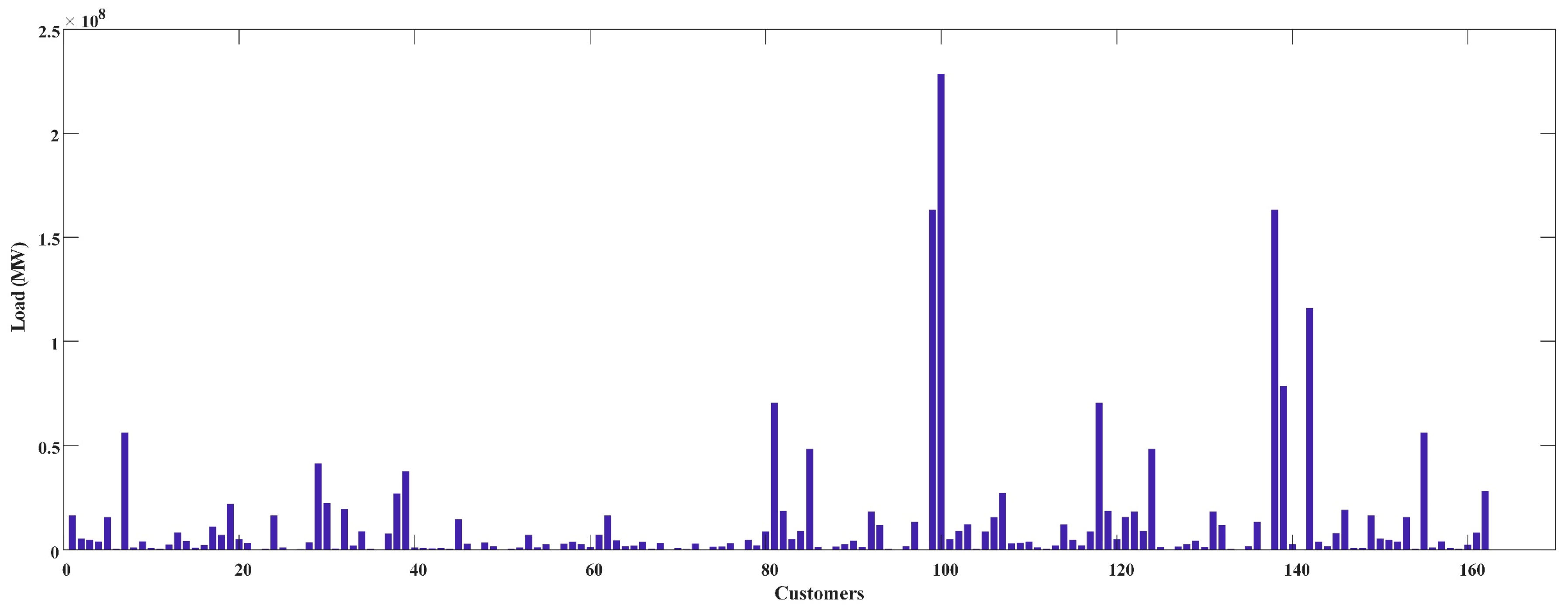
In this paper, we focus on the sector of industrial and commercial customers. Generally, since the loads of industrial and commercial consumers are larger and more consistent than those of residential customers, the DR potential of them is usually larger. The data used in this paper were collected from 162 industrial and commercial customers in a city of Jiangsu Province (China), from 1 January to 31 December in the year 2016.
The customers belong to a variety of industries. For example, industrial customers include textile manufacturing, glass manufacturing, food processing, chemical raw material manufacturing, furniture manufacturing, and so on. Commercial customers include shops, restaurants, hotels, and so on. Figure 3 shows the power consumption in 2016 of each customer. It is illustrated that, except for some large industrial customers, the annual power consumptions of the customers were mostly below MW.
4.2. CBL Performance Metrics
The baseline is compared with the actual metered electricity consumption during the DR event in order to determine the consumption reduction amount. However, to measure the performance of our method, we need to compare the calculated CBL with the actual load without the DR event.
1. Accuracy
Accuracy shows how closely the CBL approaches the actual load. The statistic chosen to measure accuracy was the median of relative root mean squared error (RRMSE).
2. Bias
Bias represents the tendency to over-or under-predict the actual load. It is measured by the median of CBL’s average relative error (ARE).
3. Overall Performance Index (OPI)
In this paper, OPI is used to evaluate the performance of CBL. It is defined as the weighted sum of accuracy and bias.
A lower OPI means that the method is more capable of predicting the CBL in the DR program. In this paper, accuracy and bias have the same weight (), which indicates the equal importance of them in the overall performance.
4.3. Clusters
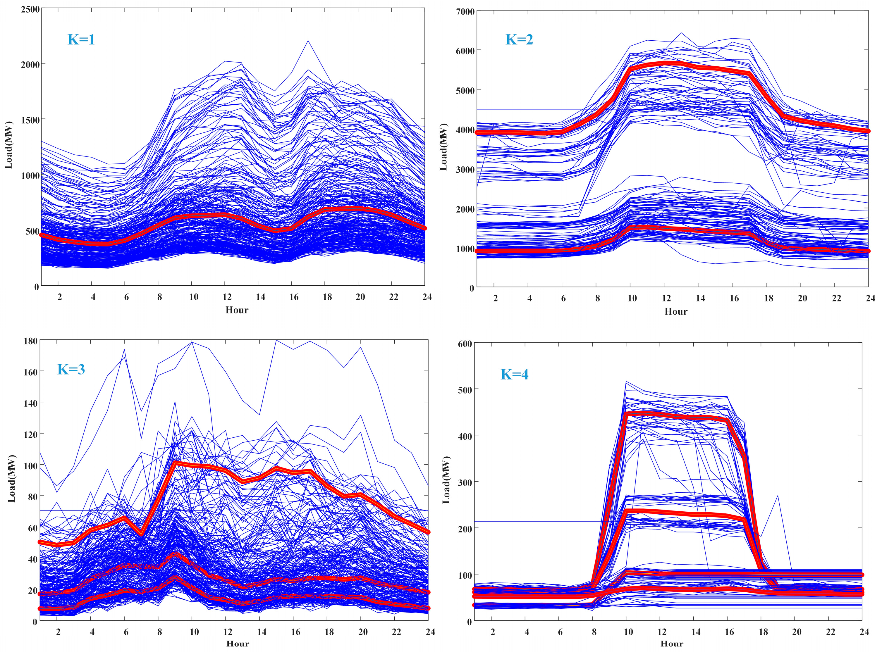
Each customer is clustered into different groups based on their load profiles. A quadratic clustering method (system clustering and fuzzy C-means clustering) is used to determine the load pattern of each customer in one year.
Figure 4 plots the load profiles of four customers with their loads of the whole year. The blue lines are the daily loads throughout the year while the red line shows the clustering center of each customer. Each customer has ‘K’ power usage patterns, where K = 1, 2, 3, and 4, respectively. It is noticeable that the value k only presents how many power usage patterns the customer has. It does not illustrate the type of power usage pattern. For example, a customer may have two power usage patterns, but it does not mean that he has two types of power usage patterns, because the two may belong to one same type.
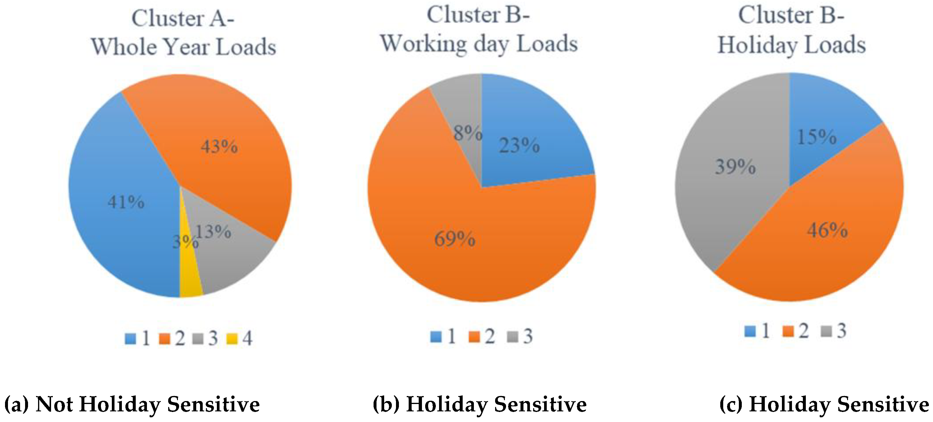
In addition, Figure 5 shows the distribution of numbers of clusters for customers with/without holiday sensitive power usage patterns. Figure 5a illustrates that, for the not holiday sensitive customers, 41% customers have one power usage pattern (blue) and 43% customers have two power usage patterns (orange), and the rest are the customers with three (grey) and four power (yellow) usage patterns. By contrast, Figure 5b,c illustrate the distribution of numbers of power usage patterns for the holiday sensitive customers. It is seen that they have three power usage patterns at most either in working days or in holidays.
4.4. Experimental Settings
To evaluate the performance of the proposed methods, various experiments are performed. The experimental outputs are the estimates of hourly load and the associated OPI. In fact, in order to evaluate the CBL performance, we need to compare them with the customer’s actual load without the DR event, and these selected 162 customers did not participate in DR event actually. Therefore, we just assume one day in each cluster as the DR event day to calculate the CBL.
4.4.1. Scenarios
There are four types of power usage patterns in total:
- Type-1: Neither holiday nor weather sensitive.
- Type-2: Only weather sensitive.
- Type-3: Only holiday sensitive.
- Type-4: Both weather and holiday sensitive.
For Type-1, the methods ‘High X of Y’, ‘Mid X of Y’, and ‘Exponential Smooth’ are used to calculate the CBL. For Type-2, since these kinds of power usage patterns are weather sensitive, we need to consider the weather adjustment after the initial CBL calculation. We use three adjustment methods- ‘multiplication adjustment’, ‘addition adjustment’, and ‘linear regression adjustment’. It is worth noting that, since these kind of power usage pattern are only weather sensitive (not holiday sensitive), we do not consider the sensitivity of holiday. For Type-3, the calculation methods are the same as Type-1, but with respect to the data selection, we need to skip the holidays. For example, when the DR event day a working day, we could only choose the working days as the calculation window in previous days. Meanwhile, it is the same in that when the DR event day is a holiday, we could only choose the holidays. Finally, for Type-4, the impact of both holiday and weather should be considered.
4.4.2. Type of DR Event Day
In this paper, cases of hypothetical DR event days are selected randomly. However, unlike what the most work done before (clustering of groups of customers), we cluster 24 points daily loads of each customer throughout the year. As a result, a customer may have ‘K’ power usage patterns during the whole year (shown as Figure 4). Therefore, it is hard to define what is the type of DR event day, since we only use the historical data to make clustering.
A common method in short-term load forecasting, called ‘selecting similar day’, is applied in this study [24,25]. There are one or two main factors that affect the value of the load. For example, when the air temperature is over 36°, the degree of air temperature is the dominant factor, while others are less. Therefore, in this algorithm, the air temperature and date distance are used to predict the ‘similar day’ of the DR event day. Therefore, the DR event day can be classified into one certain type of power usage pattern and the corresponding CBL calculation method can be applied.
4.5. Baseline Estimation Results
The correlation factor (λ) and weather sensitive factor (β) are set 0.9 and 0.5, and the length of data-selection windows are set five.
The clustering result of numbers of power usage patterns of each type is shown in Table 1. It is illustrated that most power usage patterns belong to Type-1, with their numbers over 200 on the top.
4.5.1. The Method for Each Type
Once the loads of each customer are clustered, the CBLs are calculated by using different methods. The following are the results with different methods for each type.
• Type-1
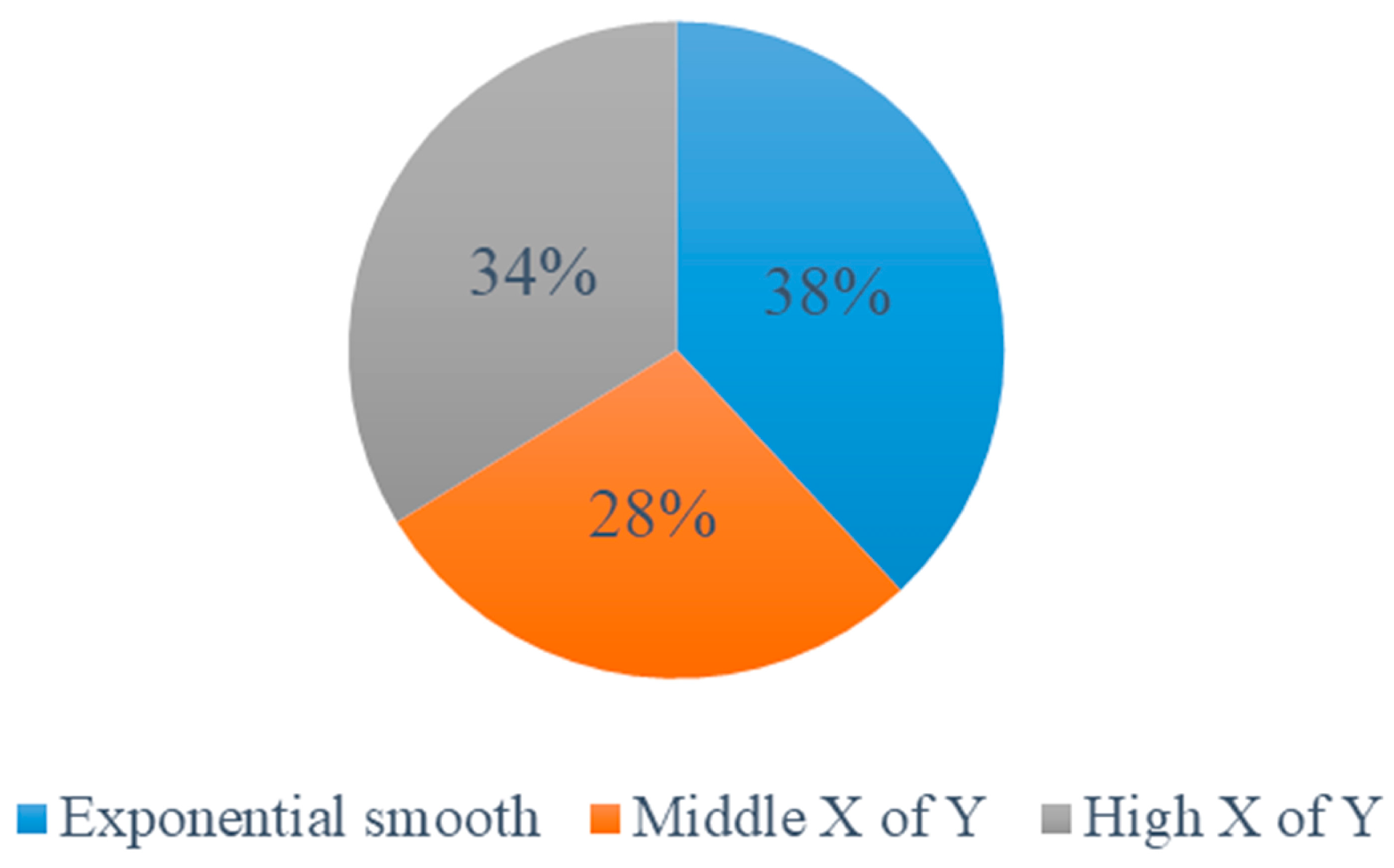
The proportion of the three methods is shown in Figure 6. It means that among the power usage patterns of Type-1, 38%, 34%, and 28% of them have the lowest error rate when using the methods ‘Exponential smooth’, ’Middle X of Y’, and ’High X of Y’, respectively. The method ‘Exponential Smooth’ is relatively preferable than the other two. This is understandable because this method weights past conversations with exponentially decreasing weights to forecast a future value, which may largely mitigate the changes of weather variability and other behavioral factors.
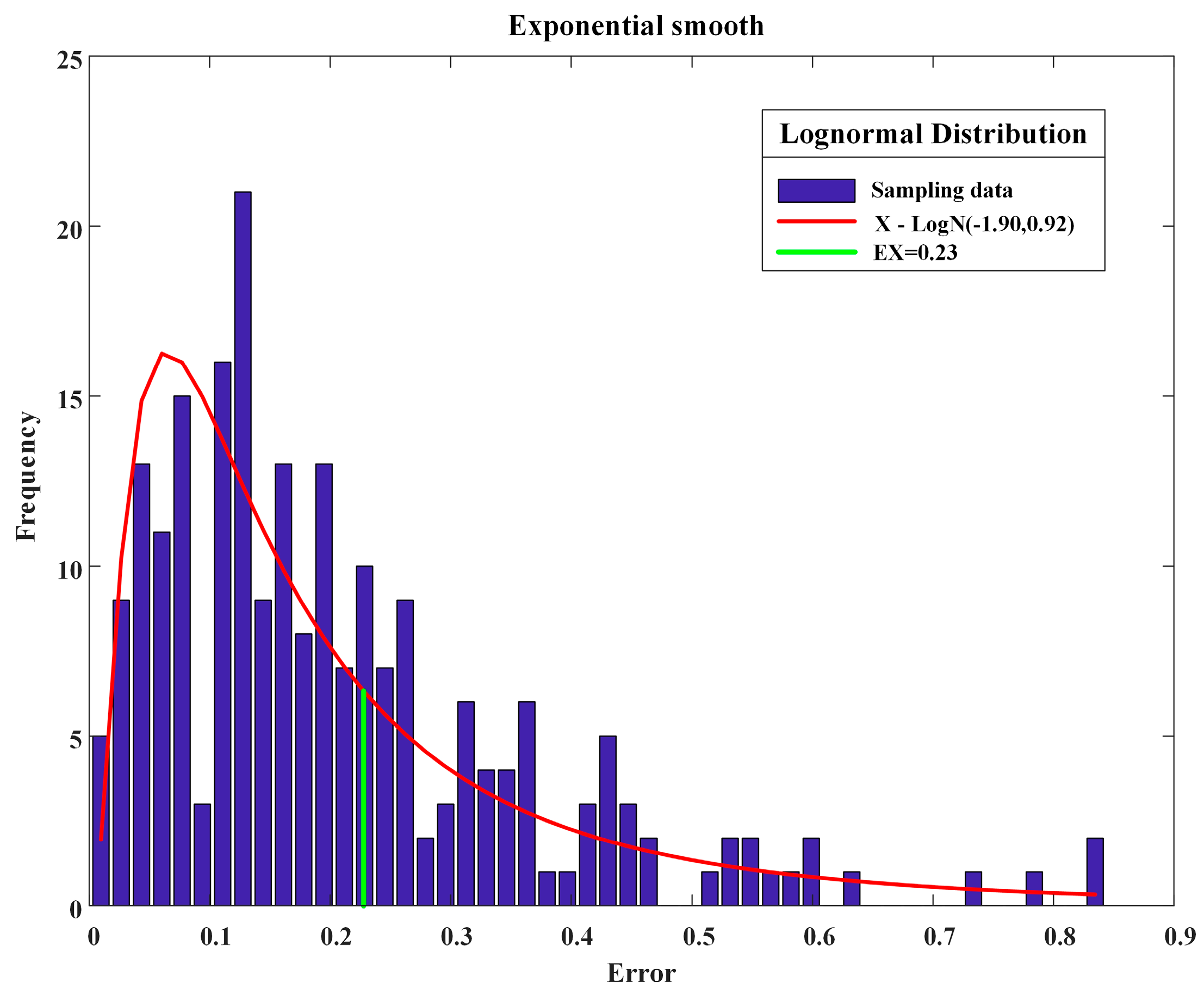
Furthermore, in order to quantitatively assess the error (OPI) calculated by the method’ Exponential smooth’, the OPI values are presented as a frequency histogram in Figure 7. It can be overserved that a fitted lognormal distribution (red line) is used to illustrate the OPI of the method using 215 samples of Type-1 and the expected value is 0.23 (green line).
• Type-2
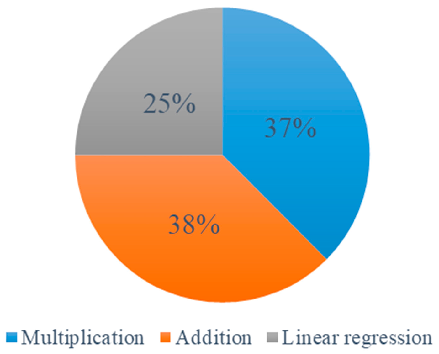
The distribution of tested adjustment methods for Type-2 is shown in Figure 8. It is illustrated that the proportion for both adjustment methods (multiplication and addition) are similar, showing that the two adjustments are equally suitable for this type of power usage patterns. By contrast, with regard to the linear regression method, since it considers the actual temperature, it should have a lower error rate than the other two, but the results come out worse. The reason for is that we use the whole year maximum load and the whole year daily average temperature to make the linear regression, and this could be inaccurate, because we do not do any correlation analysis in advance for these two variables. There can be other variable options, such maximum temperature and maximum load.
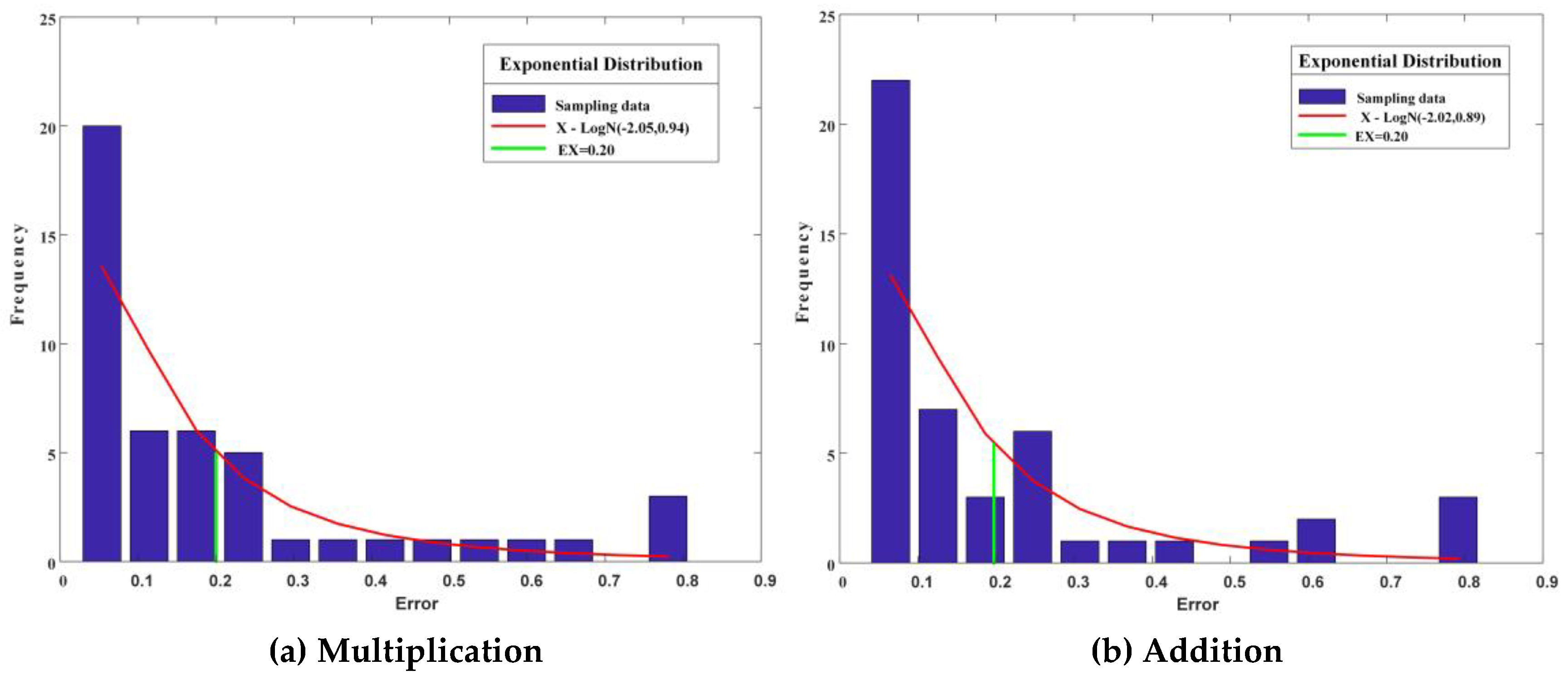
Figure 9 illustrates the errors distribution when using the multiplication adjustments and addition adjustments. We use exponential distribution (red lines) to fit the error results, and the expected value of the two are both 0.20 (green lines).
• Type-3
Since this type of power usage patterns is only holiday sensitive, it means that the power usage patterns present different characteristic compared with working days. Therefore, we need to choose the same day type as the DR event day.
The preferable calculation method is the same as Type-1 (Exponential smooth), and we do not need any adjustment.
• Type-4
Since this type of power usage patterns is both holiday and weather sensitive, we need to not only choose the same type of the previous days as the data-selection window but also calculate adjustment. We suggest that the calculation method should be the same as Type-1 and the adjustment is the same as Type-2.
4.5.2. Comparative Analysis
Since we find the preferable calculation method and adjustment method among the candidates, we still need to find out whether it is necessary to classify power usage patterns of the customer into different kinds of types. Therefore, we make some comparison, as follows.
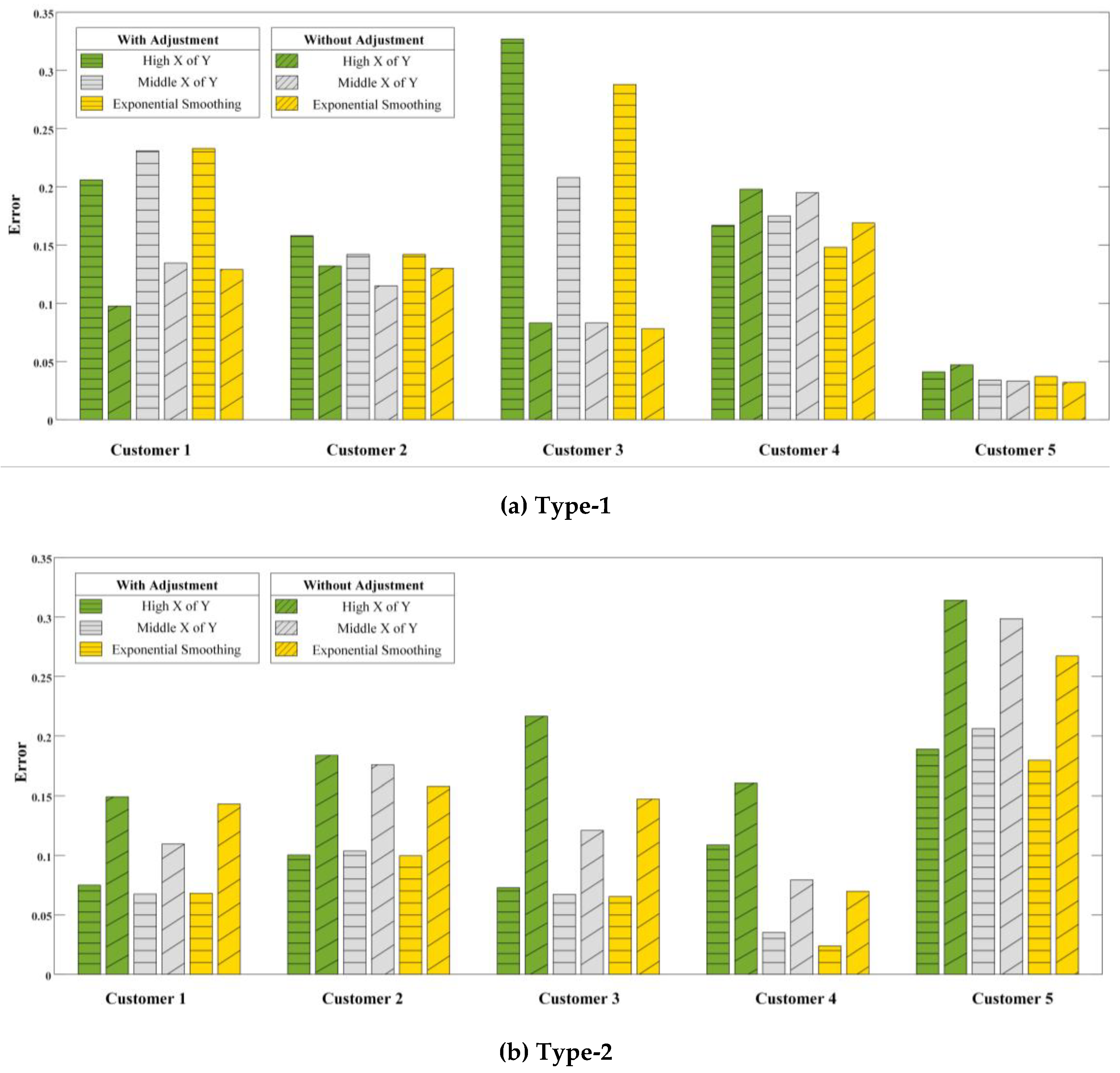
Adjustment is the method that evolves the special condition of DR program into CBL, such as weather. However, traditional methods take the adjustment no matter what the condition is, so it increases the complexity of CBL calculation. In our method, we suggest that we should consider the adjustment according to the type of customer’s power usage patterns. Therefore, we choose five representative customers with the electrical profile of Type-1 and Type-2 separately to show how the weather adjustment affects the result of CBL in Figure 10. It is noticeable that in order to focus on the difference between “with and without” adjustment, we just use the one method (addition adjustment method) to adjust the CBL.
(1) For the customers with Type-1 (neither holiday nor weather sensitive) power usage patterns, the adjustment does not have obvious improvement as the results shown. Even for some customers, the errors of the methods with the adjustment are approximately higher than those of the methods without adjustment. Therefore, we do not need to do adjustment calculation, which will simplify the process of CBL calculation. However, with regard to customer 3, it has a larger error after adjustment as compared to others. It is understandable, since we only use the addition adjustment method to adjust the initial CBL, and this method may not suitable for each customer according to the aforementioned analysis in Section 4.5.1.
(2) For the customers with Type-2 (only weather sensitive) power usage patterns, the errors generated by the three methods with adjustment are all smaller than those without. Therefore, we need to consider the adjustment after the initial CBL calculation for this type.
Same as before, we choose five representative customers with power usage patterns of Type-1 and Type-3 separately to show how the holiday-sensitive data selection affects the result of CBL. In the traditional method, we need to choose the same day type according to the DR event day. However, our proposed method suggests that we should choose the proceeding days according to the type of the power usage pattern. Figure 11 shows the comparison between the proposed method and traditional methods:
(1) For the customers with Type-1 (neither holiday nor weather sensitive) power usage patterns, there is no manifest difference between the three methods with considering the holiday-sensitive selection or not: some customers have a larger error with adjustment while some do not. As a result, we do not consider the type of the historical days when selecting the data. In other words, we can directly choose the previous days no matter that they are working days (if the DR event day is working day) or not.
(2) For the customers with Type-3 (only weather sensitive) power usage patterns, the three methods with considering the holiday-sensitive selection all show significant improvement as compared to the methods without. Therefore, we need to consider the holiday-sensitive data selection for this type.
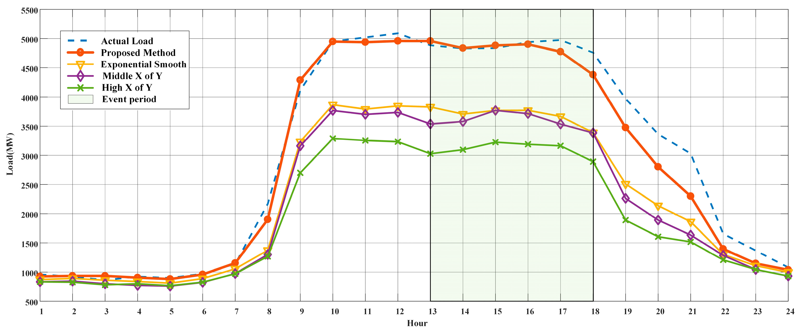
To demonstrate the effectiveness of the proposed CBL calculation approach, we randomly select one customer with Type-1 power usage pattern and then compare the performance of the proposed method with the three traditional methods in Figure 12. It is obvious that the CBL calculated by proposed method (red line) is much closer to the actual load (blue line), which means that the proposed method has a higher accuracy than the three traditional methods.
In addition, the detailed error (OPI) values of each method are shown in Table 2. It is seen that, when compared with the three traditional methods, the error rate of the proposed method reduced by 0.329, 0.228, and 0.174, respectively.
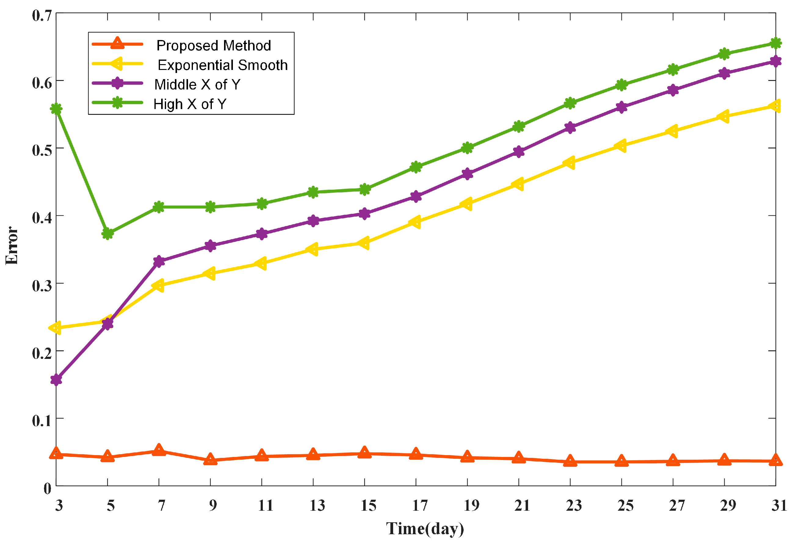
Furthermore, different length (from three to 31 days) of historical data windows are used to validate the proposed model via the sensitivity analysis in Figure 13.
It is obvious that the error of the proposed method almost remains the same as the data-selection window expands. However, for the three traditional methods, the method ‘Middle X of Y’ performs better if the number of selected days less than 5. When the data-selection window expands, the method ‘exponential smooth’ has the least error rate and the errors that are generated by three traditional methods all gradually climb. This is possibly due to the difference in historical data selection. Even if the dataset is the same, in our proposed method, the data are selected from the one clustering group after holiday sensitive analysis. By contrast, in the traditional methods, the data are directly selected from the preceding working days (or holidays) before the DR event day. Therefore, the proposed method has a higher stability and accuracy when compared to the traditional methods when the length of the data-selection window changes.
Therefore, the proposed method has a higher stability and accuracy as compared to the traditional methods when the length of the data-selection window changes.
In summary, different CBL calculation methods should be considered depending upon the customer’s multiple consumption levels. However, among all of the traditional calculation and adjustment methods, the ‘exponential smoothing model’ and ‘addition adjustment’ delivers a better result. In addition, when the data-selection window changes, the proposed calculation method is more stable and accurate than the traditional methods in terms of OPI, especially with the larger historical data.
5. Conclusions
DR programs have become popular in wholesale market in recent years. One of the common characteristics of the existing DR programs that are administered by ISO is their reliance on determined CBL. In this paper, a cluster-based CBL calculation approach is presented for individual industrial and commercial customer. It divides loads of a customer into different power usage patterns and implicitly incorporates the impact of weather and holiday into the CBL calculation. As a result, different baseline calculation approaches could be applied to each customer according to the type of his power usage patterns. In this way, the results show that the proposed method performs more stably and accurately than the traditional methods.
There are two main advantages over conventional baseline methods. Firstly, it provides accurate and stable results since we choose the data from a cluster with similar power usage pattern. Secondly, unlike traditional methods with fixed process and algorithm, the proposed method achieves personized CBL calculation according to the types of customer’s power usage patterns. However, some disadvantages to the proposed method include difficulty in creating clusters that precisely replicate the customer’s load with unique power usage patterns. This may cause the inaccurate result of CBL calculation.
Future research includes the following:
- Extending the method to residential customers to determine the applicability of the proposed methods.
- Applying the methods to data datasets from other regions in the presence of a real DR program.
- More clustering algorithms can be applied to our method to test whether the performance of CBL can be improved from our quadratic clustering method.
Author Contributions
T.S. designed the model and performed the simulations. T.S., Y.L. and J.L. analyzed the data. C.W., Q.W., B.W. and X.-P.Z. have proposed the research topic and provided materials and analysis tools. All authors contributed to the writing of the manuscript, and have read and approved the final manuscript.
Funding
This research received no external funding.
Acknowledgments
This study is supported by China Scholarship Council and British Council through the newton fund.
Conflicts of Interest
The authors declare no conflict of interest.
References
- Lee, M.; Aslam, O.; Foster, B.; Kathan, D.; Kwok, J.; Medearis, L.; Palmer, R.; Sporborg, P.; Tita, M. Assessment of Demand Response and Advanced Metering; Federal Energy Regulatory Commission: Washington, DC, USA, 2013.
- Su, C.-L.; Kirschen, D. Quantifying the effect of demand response on electricity markets. IEEE Trans. Power Syst. 2009, 24, 1199–1207. [Google Scholar]
- Ahmad, S.; Ahmad, A.; Naeem, M.; Ejaz, W.; Kim, H. A Compendium of Performance Metrics, Pricing Schemes, Optimization Objectives, and Solution Methodologies of Demand Side Management for the Smart Grid. Energies 2018, 11, 2801. [Google Scholar] [CrossRef]
- Chao, H.-P. Demand response in wholesale electricity markets: The choice of customer baseline. J. Regul. Econ. 2011, 39, 68–88. [Google Scholar] [CrossRef]
- Conejo, A.J.; Morales, J.M.; Baringo, L. Real-time demand response model. IEEE Trans. Smart Grid 2010, 1, 236–242. [Google Scholar] [CrossRef]
- Chen, W.; Wang, X.; Petersen, J.; Tyagi, R.; Black, J. Optimal scheduling of demand response events for electric utilities. IEEE Trans. Smart Grid 2013, 4, 2309–2319. [Google Scholar] [CrossRef]
- Zhang, Y.; Chen, W.; Xu, R.; Black, J. A cluster-based method for calculating baselines for residential loads. IEEE Trans. Smart Grid 2016, 7, 2368–2377. [Google Scholar] [CrossRef]
- Park, S.; Ryu, S.; Choi, Y.; Kim, J.; Kim, H. Data-Driven Baseline Estimation of Residential Buildings for Demand Response. Energies 2015, 8, 10239–10259. [Google Scholar] [CrossRef] [Green Version]
- PJM Empirical Analysis of Demand Response Baseline Methods. PJM Load Manage. Task Force; KEMA Inc.: Clark Lake, MI, USA, 2011.
- Day-Ahead and Real-time Market Operations. PJM Manual 11: Energy & Ancillary Service Market Operations. 2017. Available online: https://www.pjm.com/~/media/documents/manuals/m11.ashx (accessed on 1 November 2017).
- Qu, D.; Wu, W.; Jiang, D.; Chen, G. Calculation method of radial basis function neural network based on user demand side response baseline load. Electron. Test 2014, 2, 26–30. (In Chinese) [Google Scholar]
- Liu, G.; Gao, Y.; Wang, L. Baseline load calculation with considering customer different electrical characteristics. Power Demand Side Manag. 2016, 33, 17–22. [Google Scholar]
- Baylis, P.; Cappers, P.; Jin, L.; Spurlock, A.; Todd, A. Go for the Silver? Evidence from field studies quantifying the difference in evaluation results between “gold standard” randomized controlled trial methods versus quasi-experimental methods. In Proceedings of the ACEEE Summer Study on Energy Efficiency in Buildings, Asilomar, CA, USA, 21–26 August 2016. [Google Scholar]
- Mohajeryami, S.; Doostan, M.; Asadinejad, A.; Schwarz, P. Error analysis of customer baseline load (CBL) calculation methods for residential customers. IEEE Trans. Ind. Appl. 2017, 53, 5–14. [Google Scholar] [CrossRef]
- Wijaya, T.K.; Vasirani, M.; Aberer, K. When bias matters: An economic assessment of demand response baselines for residential customers. IEEE Trans. Smart Grid 2014, 5, 1755–1763. [Google Scholar] [CrossRef]
- Fallah, S.N.; Deo, R.C.; Shojafar, M.; Conti, M.; Shamshirband, S. Computational Intelligence Approaches for Energy Load Forecasting in Smart Energy Management Grids: State of the Art, Future Challenges, and Research Directions. Energies 2018, 11, 596. [Google Scholar] [CrossRef]
- Wang, Y.; Chen, Q.; Sun, M.; Kang, C.; Xia, Q. An ensemble forecasting method for the aggregated load with sub profiles. IEEE Trans. Smart Grid 2018, 9, 3906–3908. [Google Scholar] [CrossRef]
- Huang, J.; Li, Y.; Liu, Y. Summer daily peak load forecasting considering accumulation effect and abrupt change of temperature. In Proceedings of the Power and Energy Society General Meeting (PES), San Diego, CA, USA, 22–26 July 2012; Volume 6, pp. 1–4. [Google Scholar]
- Gao, C.; Li, Q.; Su, W.; Li, Y. Temperature correction model research considering temperature cumulative effect in short-term load forecasting. Trans. China Electrotech. Soc. 2015, 4, 242–248. (In Chinese) [Google Scholar]
- Grimm, C.; Energy, D.T.E. Evaluating baselines for demand response programs. In Proceedings of the AEIC Load Research Workshop, San Antonio, TX, USA, 25–27 February 2008. [Google Scholar]
- Faria, P.; Vale, Z.; Antunes, P. Determining the adjustment baseline parameters to define an accurate customer baseline load. In Proceedings of the Power and Energy Society General Meeting (PES), Vancouver, BC, Canada, 21–25 July 2013; pp. 1–5. [Google Scholar]
- Yamaguchi, N.; Han, J.; Ghatikar, G.; Kiliccote, S.; Piette, M.A.; Asano, H. Regression models for demand reduction based on cluster analysis of load profiles. In Proceedings of the Sustainable Alternative Energy (SAE), Valencia, Spain, 28–30 September 2009; pp. 1–7. [Google Scholar]
- Hatton, L.; Charpentier, P.; Matzner-Løber, E. Statistical estimation of the residential baseline. IEEE Trans. Power Syst. 2016, 31, 1752–1759. [Google Scholar] [CrossRef]
- Li, C.; Li, X.; Zhao, R.; Li, J.; Liu, X. A novel algorithm of selecting similar days for short-term power load forecasting. Autom. Electr. Power Syst. 2008, 9, 18. (In Chinese) [Google Scholar]
- Sun, X.; Luh, P.B.; Cheung, K.W.; Guan, W.; Michel, L.D.; Venkata, S.; Miller, M.T. An efficient approach to short-term load forecasting at the distribution level. IEEE Trans. Power Syst. 2016, 31, 2526–2537. [Google Scholar] [CrossRef]
Figure 1.
Relationship among predicted customer baseline load (CBL), actual load, and load reduction.
Figure 1.
Relationship among predicted customer baseline load (CBL), actual load, and load reduction.

Figure 2.
Framework of baseline calculation considering customer’s multiple power usage patterns.

Figure 3.
The annual power consumption of each customer.

Figure 4.
Numbers of clusters of each customer.

Figure 5.
Distribution of numbers of clusters for two types of power usage patterns.

Figure 6.
Distribution of tested methods for the Type-1.

Figure 7.
Estimation error distribution of method-‘Exponential smooth’ for Type-1.

Figure 8.
Distribution of tested adjustment methods for Type-2.

Figure 9.
Estimation error distribution of two adjustment methods for Type-2.

Figure 10.
The contrast of the tested methods with considering weather sensitivity or not.

Figure 11.
The contrast of the three methods considering holiday sensitivity or not.

Figure 12.
CBL calculation: the comparison among proposed method and traditional methods.

Figure 13.
Error in CBL with respect to changes in data-selection window.


Table 1.
Numbers of power usage patterns in each type.
| Type | Type-1 | Type-2 | Type-3 | Type-4 |
|---|---|---|---|---|
| Numbers | 215 | 37 | 34 | 14 |
Table 2.
Error (Overall Performance Index (OPI)) per method.
| Methods | Proposed Method | High X of Y | Middle X of Y | Exponential Smooth |
|---|---|---|---|---|
| Error (OPI) | 0.064 | 0.393 | 0.292 | 0.238 |
© 2018 by the authors. Licensee MDPI, Basel, Switzerland. This article is an open access article distributed under the terms and conditions of the Creative Commons Attribution (CC BY) license (http://creativecommons.org/licenses/by/4.0/).
Share and Cite
MDPI and ACS Style
Song, T.; Li, Y.; Zhang, X.-P.; Li, J.; Wu, C.; Wu, Q.; Wang, B. A Cluster-Based Baseline Load Calculation Approach for Individual Industrial and Commercial Customer. Energies 2019, 12, 64. https://doi.org/10.3390/en12010064
AMA Style
Song T, Li Y, Zhang X-P, Li J, Wu C, Wu Q, Wang B. A Cluster-Based Baseline Load Calculation Approach for Individual Industrial and Commercial Customer. Energies. 2019; 12(1):64. https://doi.org/10.3390/en12010064
Chicago/Turabian StyleSong, Tianli, Yang Li, Xiao-Ping Zhang, Jianing Li, Cong Wu, Qike Wu, and Beibei Wang. 2019. "A Cluster-Based Baseline Load Calculation Approach for Individual Industrial and Commercial Customer" Energies 12, no. 1: 64. https://doi.org/10.3390/en12010064
Note that from the first issue of 2016, this journal uses article numbers instead of page numbers. See further details here.