Electricity Price Forecasting in the Danish Day-Ahead Market Using the TBATS, ANN and ARIMA Methods


Department of Business Development and Technology, Aarhus University, Birk Centerpark 15, 7400 Herning, Denmark
*
Author to whom correspondence should be addressed.
Energies 2019, 12(5), 928; https://doi.org/10.3390/en12050928
Submission received: 13 January 2019
/
Revised: 4 March 2019
/
Accepted: 5 March 2019
/
Published: 10 March 2019
(This article belongs to the Special Issue Demand Response in Electricity Markets)
Abstract
:In this paper day-ahead electricity price forecasting for the Denmark-West region is realized with a 24 h forecasting range. The forecasting is done for 212 days from the beginning of 2017 and past data from 2016 is used. For forecasting, Autoregressive Integrated Moving Average (ARIMA), Trigonometric Seasonal Box-Cox Transformation with ARMA residuals Trend and Seasonal Components (TBATS) and Artificial Neural Networks (ANN) methods are used and seasonal naïve forecast is utilized as a benchmark. Mean absolute error (MAE) and root mean squared error (RMSE) are used as accuracy criterions. ARIMA and ANN are utilized with external variables and variable analysis is realized in order to improve forecasting results. As a result of variable analysis, it was observed that excluding temperature from external variables helped improve forecasting results. In terms of mean error ARIMA yielded the best results while ANN had the lowest minimum error and standard deviation. TBATS performed better than ANN in terms of mean error. To further improve forecasting accuracy, the three forecasts were combined using simple averaging and ANN methods and they were both found to be beneficial, with simple averaging having better accuracy. Overall, this paper demonstrates a solid forecasting methodology, while showing actual forecasting results and improvements for different forecasting methods.
1. Introduction
Electricity is an energy commodity much different from oil, natural gas, coal and likes because it is not easily storable locally in large quantities. Storing electricity at a grid-scale is a desired grid characteristic, however it is not widely used because it is not economically feasible and totally uncompetitive at the moment. In addition, the electricity on the grid should be perfectly balanced at all times to prevent outages and other issues.
Electricity markets in Europe started being liberalized in the beginning of 1990s [1]. With the adoption of EU market liberalization directives, electricity markets in EU became completely liberalized in the first decade of 2000s. Before the liberalization, markets were mostly controlled by governments and their agencies. With the liberalization of the markets, electricity generation, supply, transmission and distribution became competitive activities, achieving reductions in price [2] towards the goal of low carbon areas, mainly by mergers, privatisation, and asset acquisitions [3,4,5]. Competitive programmes were initiated—mainly by the EU—aiming at increasing countries’ interconnectivity developing new power and energy markets.
Many actors are present in the markets such as producers, traders, transmission system operators (TSOs). In liberalized electricity markets, electricity is traded in different types of markets. The Denmark electricity market is a part of the Nordpool Power Market which aims to integrate European Energy Markets therefore Denmark follows electricity trading as per Nordpool regulations [6].
Electricity price forecasting is a vital activity for the members of the markets in order to take decisions and maximize their profits [7,8,9]. Due to the nature and the rules of the electricity markets, which will be discussed in the next section, forecasting is necessary activity to take part in the trading process [10,11].
Nordpool
Nordpool is an initiative owned by different European TSOs participating in the market, including the Danish TSO Energinet. It is one of the oldest and well established power exchanges in the world [7]. Trading at Nordpool happens in the day-ahead markets and the intraday markets.
The day-ahead market is where the majority of trading happens in terms of volume. Bids for 24 h the next day are submitted before 12:00 CET the day before, meaning that a forecasting range of 24 h is used, starting from 12 h ahead. When the market prices are calculated, then trade volumes are fixed. This means minimum 36 h ahead should be forecast in order to participate in the bidding. The bids concern 1 h intervals. Some of the key factors that play a significant role are bottlenecks, transmission capacities, volumes to meet demand, congestion, and different area prices.
The main role of the intraday market is to keep the balance in the grid using a shorter bidding interval then day-ahead markets. The fluctuations might happen due to many different factors such as excessive winds, malfunctions in a production plant or an unexpected change in demand. Trading in the Nordpool intraday market happens continuously until one hour before delivery (Nordpool Website). The role of the intraday market is to assist the day-ahead one towards securing matching demand with supply. Regulations at finer intervals are covered by the local TSO, which is Energinet in Denmark’s case [7,12].
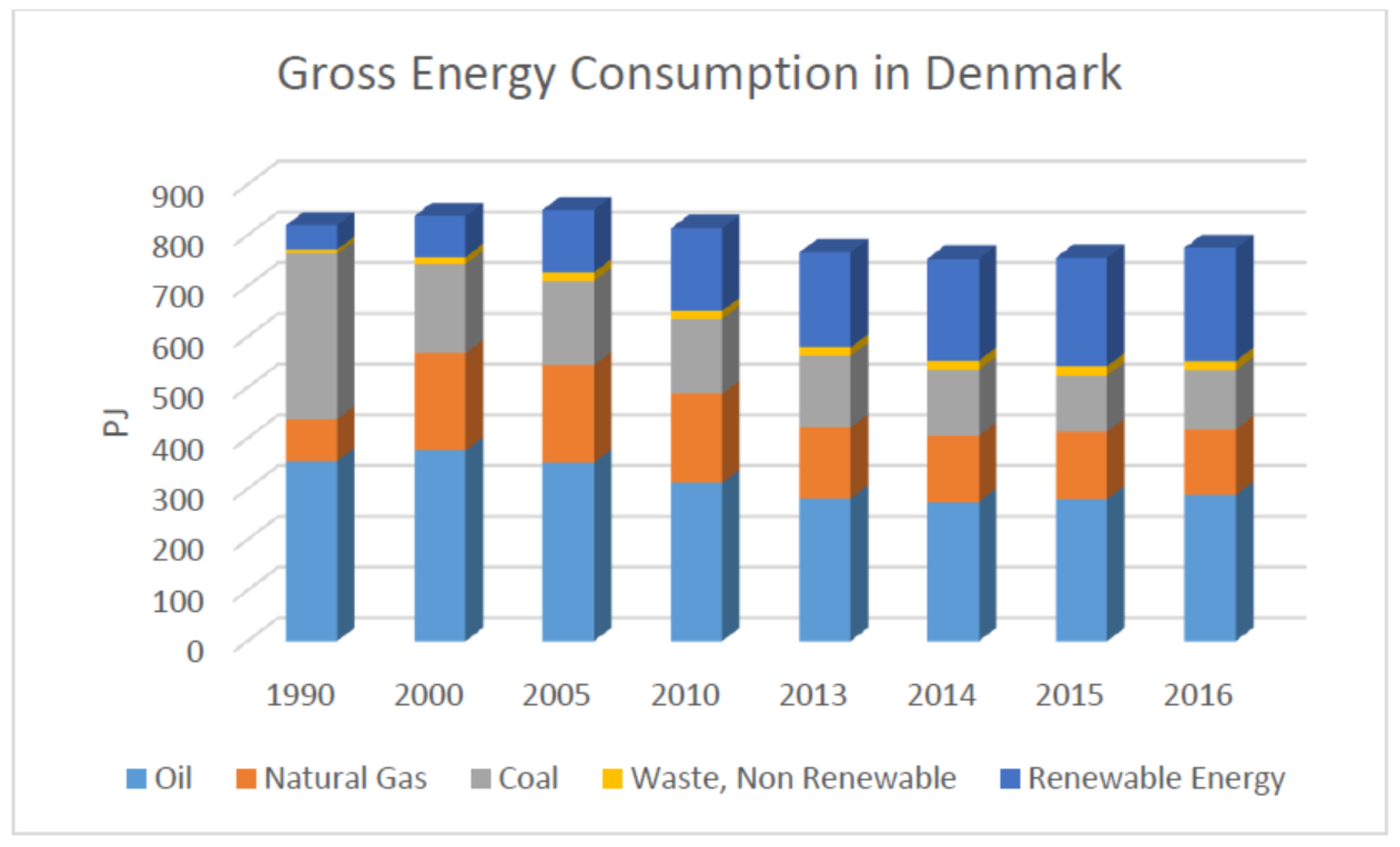
The electricity market in Denmark is dominated by the increasing penetration of renewable energy, which is also highlighted by the Danish Government’s plans to become independent from fossil fuels by 2050 [13]. Figure 1 shows that coal consumption has decreased a lot over the last three decades, with renewable energy use increasing. Changes in oil and natural gas seem marginal in comparison. The data also shows that oil, natural gas, and coal, along with renewable energy, are important energy consumption components and they should be considered in the price forecasting model, if possible.
In 2016, 38% of electricity consumption in Denmark was provided by wind energy alone [14], and this percentage became even higher for 2017, making it the largest component of the renewable energy category. Due to the uncontrolled and random nature of wind power, it may at times create imbalances and price jumps. Unlike power plants, where the electricity production is scheduled and controlled according to the requirements in the grid, wind power may at times act against the needs of the grid. Wind energy has an important effect on electricity prices therefore, it should be included in the forecasting model as well. The electricity grid in Denmark is divided into two parts: DK1 is the western part of Denmark, including Fyn and Jutland, and DK2 is the eastern part covering Zealand and Islands [14].
2. Research
2.1. Research Goals
The outcome of the research will be an artifact, a computer program that forecasts electricity prices given historical data and other required inputs. Multiple models will be implemented for comparison and it will be used to decide which is better as this is a recommended practice [15]. Realizing the forecasts, further analysis and possible improvements will be discussed and implemented. The first goal of the project can be defined as determining the best individual forecasting method out of the applied forecasting models. The second goal is to suggest and apply ways to improve the individual forecasts, and the third goal is to demonstrate a solid methodology that can be applied to different forecasting problems [16].
2.2. Methodology
Understanding the regulations of electricity markets and Denmark’s special conditions is very important in order to correctly identify price drivers and relevant variables. These are discussed in detail throughout the paper as they contain a lot of information and assumptions, and constitute an integral part of the research. The availability and the collection of the data is also crucial as it affects the implementability of the models.
After collecting the data, preliminary data analysis is required to understand the data better. This will enable us to find good models that fit our data well. For the data analysis, tools such as correlation graphs, autocorrelation functions, comparative variable analysis, decomposition and residual analysis will be used. First the data to be used in the forecasting will be analysed using statistical tools and patterns for seasonality will be checked using autocorrelation analysis. Then the data will be decomposed and further analysis will be done on patterns and residuals. For variable analysis correlation scatterplots will be used as the main tools. Each variable and its possible effects on the data will be discussed briefly.
After setting up the model, the input data will be divided into two parts, one for training the model and one for testing the forecasts. The forecasting range will be 24 h with an hourly frequency. To include a full year of training data as a minimum, 2016 data will be taken as the training period. 2017 prices will be forecasted as an expanding forecast for 212 days, which is from the start of January to end of July. Expanding forecast means that after forecasting the next 24 h, that raw data is included to our training period for forecasting the day after. As mentioned by [7,17,18] short and carefully selected test periods do not give any information regarding the performance of the forecasts as they are ignoring special days, holidays and general price variations. Therefore, a 7-month period for forecasting will be used for more objective and better assessment of forecasting models.
For the evaluation of the forecasts, scaled error models will be preferred over percentage error models as percentage models can yield infinite error when the actual electricity prices are 0 DKK/MWh, making them unreliable. The reader should keep in mind that the performance of the models should only be compared for the same set of data of the same time using the same error calculation model. Also for evaluation simpler forecasting methods can be used as benchmarks. One model that will be used is the seasonal naïve method, which is basically assuming that the price to be forecasted is similar to the previous period’s prices, such as previous week.
After comparing the error values and evaluating the forecasts, ways to improve the forecasting performance of the models will be investigated using backwards feature elimination. This tool will provide the removal of variables that are irrelevant to the forecasts. Then an attempt at combining the forecasts in order to gather more accurate forecasts will be realized. The paper will be finalized with conclusion, evaluation of the study and suggestions for further studies.
2.3. Forecasting Methodology
Forecasting can be defined as estimating future unknown values in an educated and systematic way using available data. As the values of the data that is to be forecasted is unknown, there are different possible values and the forecaster aims to find the most probable value(s). In case the forecast is used to obtain a single value as the most probable value the forecast is called a point forecast, whereas a probability forecast contains a range of values with the prediction intervals and densities [19]. In this research point forecasts will be used as they are simpler and easier to interpret.
There are a variety of tools and methods for forecasting. It is important for a forecaster to be able to spot the right tools considering the data and the forecast span. To achieve this the problem should be defined clearly and relevant data should be collected. To achieve this task the following steps mentioned by [17] will be followed. These steps are as follows: problem definition, gathering information, preliminary analysis, choosing and fitting models, and using and evaluating a forecasting model.
The forecasting problem of the project is to forecast day-ahead electricity prices from Denmark Jutland (including Fyn) region, commonly referred to as DK1 or DKWest in Energinet or Nordpool sources. The forecasting span has been selected as 24 h to simplify and imitate the actual bidding that takes place in Nordpool. As the aim is to forecast hourly prices using more frequent data than hourly will not be necessary. Data from 2016 will be used as training data and the first seven months of 2017 will be forecasted.
Historical data regarding electricity prices is available online at Nordpool website. For the explanatory variables different sources are being used. Temperature data is provided by Energinet for the Tange location. As this is a central location in Jutland and knowing Denmark is mostly flat it is assumed that this temperature portrays a good average for the region and the temperature across the region is highly positively correlated.
Other explanatory variables such as consumption prognosis, production prognosis, wind power prognosis and hydro reserve levels are provided by Nordpool and Energinet. Since they have direct access to the producers, and the users they are seen as highly credible and reliable sources.
Oil and natural gas prices are taken from Fred series [20]. For oil, “Crude Oil Prices: Brent—Europe” and for natural gas, “Henry Hub Natural Gas Spot Price” data sets are taken into consideration.
Data obtained from Fred and hydro reservoir data are weekly data where the data are copied to the corresponding values for each hour of the week. It is assumed that this data frequency is suitable these variables are not very volatile or have high variance in short time and possibly their effects are not seen hourly or daily in the corresponding data. Other data mentioned are collected and used as hourly data.
Hydro reservoir level is derived from the data collected from Nordpool. Following equation (Equation (1)) is used in order to obtain the data, where HRL is the hydro reservoir level, NL is the amount of water in reservoirs in Norway, SL is the amount of water in reservoirs in Sweden and FL is the amount of water in Finish reservoirs. NC, SC, and FC correspond to the total available water capacities in respective countries. Using the equation a value between 0 and 1 is reached, where 1 means that the reservoirs are full and 0 means that they are empty:
Two dummy variables are also considered in our data sets, one for weekdays and one for holidays including the weekends. Two sources are used to spot the holidays (the Office Holidays and the Public Holidays) [21,22] in order to crosscheck the validity of the data. Also, weekends that are combined with the holidays are included in the holiday data set as it is assumed that they might exhibit similar behaviours to holidays than normal weekends. There is one variable for weekdays and weekends and one for holidays and non-holidays. Therefore for the holiday variable: (a) for holiday the value is ”1”, and (b) for non-holiday the value is ”0”. For the weekday variable: (c) for a weekday the value is “0” and for the weekend the value is “1”. Using coal prices was also planned as coal constitutes a significant portion of the energy consumption however, suitable data in this regard was not accessible and therefore coal prices were omitted from the forecasts. The reason why coal prices were not attainable is because coal has many different types depending on British thermal units (BTU) and maybe it is not traded in spot markets and rather traded privately.
A large number of researchers used dummy variables to explain seasonal variables, such as the day of the week [23,24]. The latter of the two papers test consumption and production prognosis as variables. Other researchers [25] use system loads, fuel prices, seasonal variables stressing that available hydro energy and fuel prices are variables that could be used if, and when, data are present. Other researchers took into account the natural gas prices as explanatory variable. They did also test temperature, but was found of low correlation [26]. Others like [27] test wind prognosis, however, it was the link to price that was mainly proven.
One very important price driver is the planned or unexpected changes in production such as planned maintenance or unexpected problems in a production plant. This information is present in Nordpool website, under the name Remit Urgent Market Messaging (UMM) however a method to make the information useful and usable is needed before incorporating it into a model. This method should compose of two parts, one to filter and download the required data and the second one to convert the data into usable quantitative information before incorporating it into the models. Due to the time limitations of the project, these data are excluded from the models.
One other factor that has an effect on the prices is the transmission of electricity. Transmission lines are used to convey electricity and because electricity is mostly brought from where the production is high and prices are low to high consumption regions, the transmission lines have an effect to smooth and bring the prices closer to each other. When the transmission capacity of the lines are close the local production and consumption becomes more important therefore the prices tend to have more spikes. As the transmission lines and the interaction between regions and markets are very complicated and not straightforward to incorporate into a regression model, they are excluded from our models as well.
Reserve margin is a metric that relates available production capacity to consumption and in some markets it seems to be a reliable predictor for spike forecasting [7]. These data are not present in Nordpool or Energinet however if they were present, they should have been included in the model as they could have contributed when the prices are harder to forecast, at high volatility.
2.4. Methodology and Tools Used
Three models were practically used: ARIMA, TBATS and ANN. An analytical description of the models can be found below.
2.4.1. ARIMA Model
ARIMA models are one of the most frequently used and recognized forecasting models. In order to use a certain data with ARIMA, the data has to be stationary first. This means that the trend and the seasonality of the data should be eliminated before applying the ARIMA model. ARIMA model consists of three parts, autoregressive (AR), integral, and moving average (MA). AR refers to using the lagged inputs to forecast the future data. Integral refers to differencing needed to make the data stationary. MA is similar to AR, as it is used to forecast the error using the past (lagged) errors. [17]. With this brief explanation at hand, ARIMA(p,d,q) model means that the data is differenced d times, p lagged points are used in AR and q lagged errors are used in MA. An ARIMA(p,0,q) model can also be referred to as ARMA(p,q) model as there is no differencing involved. The regression with ARMA errors with one external regressor can be defined as follows where both equations are determined simultaneously:
where is the white noise, is the external regressor at time t, B is the coefficient regarding the external regressor, is the residue from the fit and is modelled as an ARMA process.
The input variables can be differenced as many times as needed in order to make the data stationary, and the model can be extended to include more external regressors. The coefficients of the equations can be solved using maximum likelihood estimation (MLE) [17].
The function “auto.arima” is included in the forecasting package of R, used to make an ARIMA fit using the Hyndman-Khandakar algorithm to choose the model parameters [28]. The algorithm first uses the Kwiatkowski-Phillips-Schmidt-Shin [29] unit root test to identify if the series is stationary and to choose the correct d parameter. Then various p and q parameters are heuristically tested and selected in order to minimize the corrected Akaike information criterion (AIC). The function is not fully automated, and the outliers have to be cleaned, and if there is variance Box-Cox transformation should be applied before using auto.arima. The fitting is done using MLE. After the fit, the results should be examined for irregularities such as autocorrelation. When using the auto.arima function with exogenous variables, the function works as a regression model with ARMA errors. A detailed explanation of the procedure and best practice can be found in [17].
2.4.2. TBATS Model
TBATS model is an exponential smoothing method, which includes Box-Cox Transformation (method for non-linear data), ARMA model for residuals, and the Trigonometric Seasonal. The trigonometric seasonality expression can significantly reduce model parameters at high seasonality frequencies and at the same time offer the model plasticity to compromise with complex seasonality. On the negative side, the computation cost is significantly large if the data files are huge, however among the strengths that this model has are: (a) the option of implementing a multi-seasonality analysis without too many parameters, (b) it can work under non-integer seasonality, (c) it can work under high frequency data (and this is one of the reasons it was selected) [30].
2.4.3. ANN Models
ANN models have been widely used in the literature and seen to provide satisfactory forecasting accuracy. ANNs are machine learning systems that resemble the neural networks of biological structures [30,31]. One important aspect of ANNs is that, by having a hidden layer, one can achieve a nonlinear output function. In a feedforward neural network, the information is carried forward from one layer to the next layers and not backwards. The weights of the connections are updated in each run, which is called the training of the network. A DNN represents an ANN with two or more hidden layers. A fully connected neural network refers to an ANN that each node is connected to all the nodes in the next layer with a specific weight [17]. Each ANN is comprised of an input layer, an output layer, and nodes in the associated layers. Optionally, single or multiple hidden layers can also be present. Each node sums its inputs multiplied by the respective weight and the summation is transferred to an activation function with a bias.
The result of the activation function is the output of the node. During training of the conventional ANN, the weights of the inputs and bias are updated in order to minimize the error. One common algorithm to optimize the weights is called the backpropagation algorithm. In this case of forecasting, the number of input nodes is equal to the number of variables that are inputted into the system. The output node is always one, which gives the point forecast result. The number of hidden layers and the nodes in each layer will depend on the model and heuristics testing. An ANN without a hidden layer will be analogous to a linear regression model. Adding more layers and nodes will enable the model to perform non-linear and more complex tasks, whereas adding too much of them may cause overfitting and cause the model to lose its generalization ability. In the case of overfitting, the noise in the data is mistakenly interpreted as information and is contained in the data [17].
3. Preliminary Data Analysis
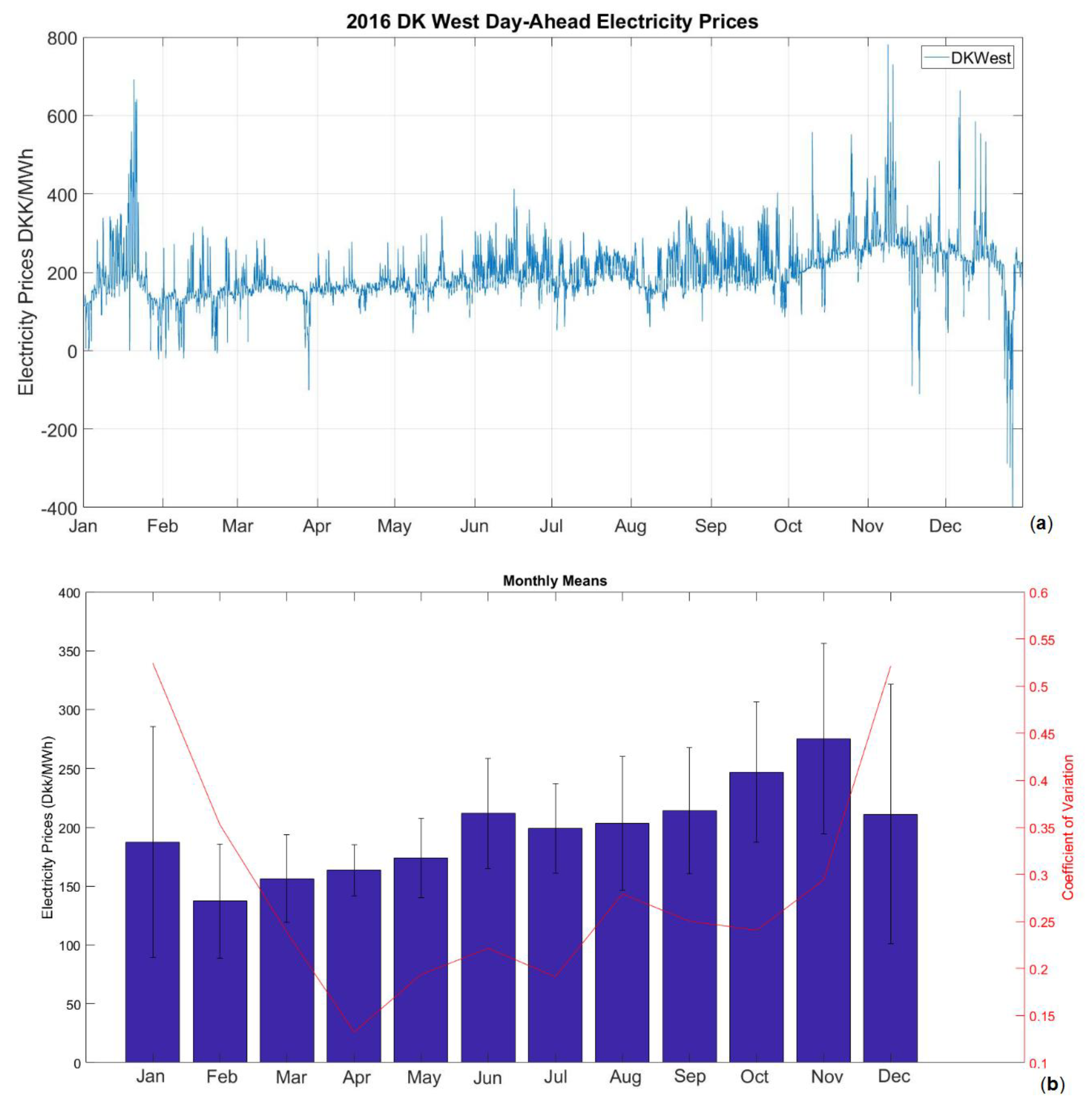
Data should be analysed first in order to select an appropriate forecasting model. After deciding on the model, it can be implemented with training data set and evaluated according to the results received with the test data. The raw data from Figure 2 were evaluated.
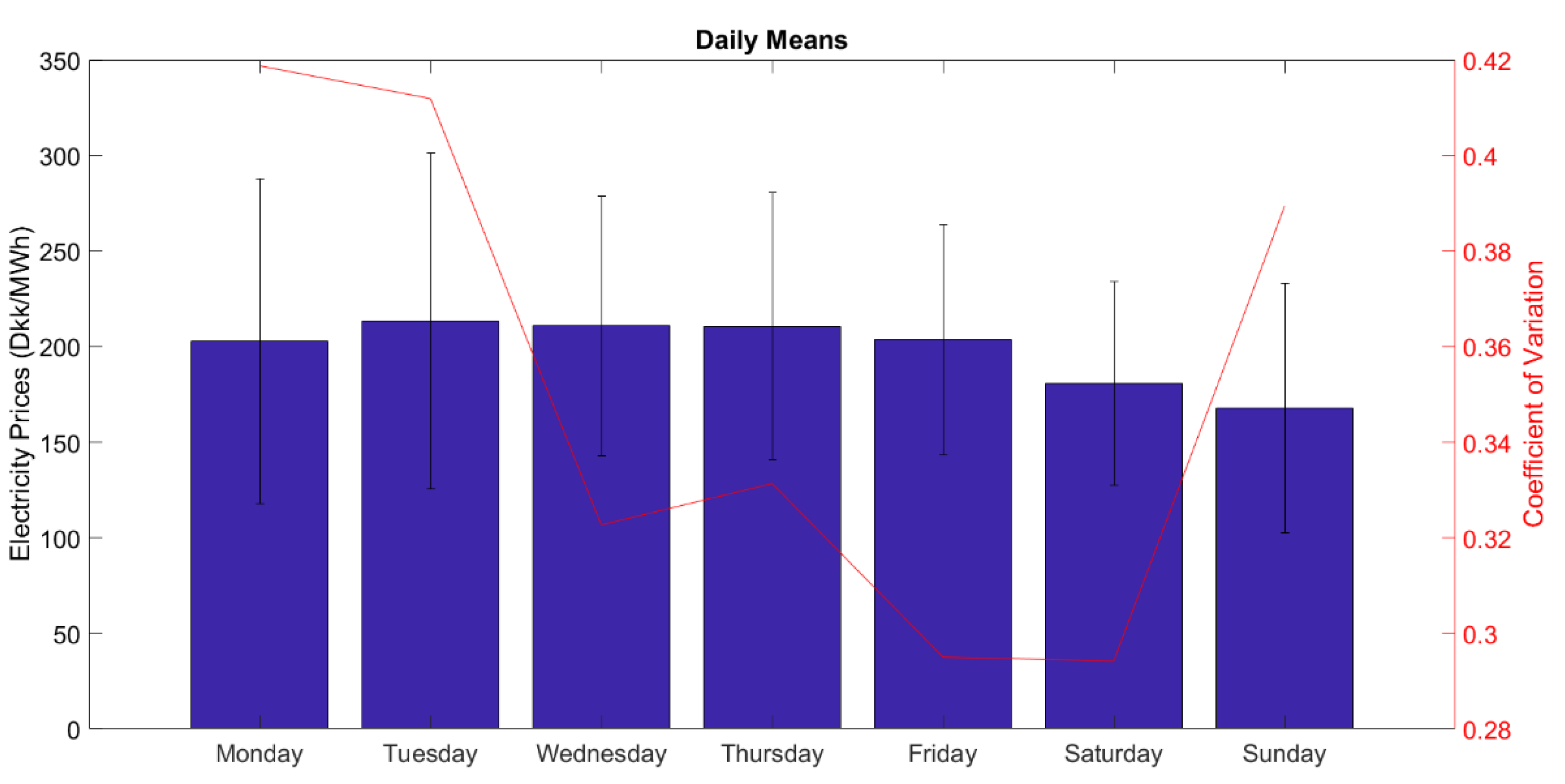
At the end of the December there is a noticeable negative jump. Looking at the dates it can be assumed that this period corresponds to Christmas and due to the holiday, there is a lower demand creating a fall in the prices. A similar but much smaller effect can be seen at the end of March, which may be a similar effect caused by Easter. A rising trend beginning with October until February can also be seen and this effect can be due to colder weather creating increased consumption due to heating requirements. Other noticeable patterns are seen with spikes in January and November followed by negative jumps in November. Figure 2b shows monthly means for the data shown in Figure 1 with the standard deviation bars. It can be seen from Figure 2 that each month the mean price is changing with highest prices in November and lowest prices in February. The standard deviation is highest in December and January possibly due to holidays mentioned. Standard deviation is lowest in April. The yearly seasonal effect can be seen more clearly just by looking at the monthly means. Looking at Figure 3, which shows daily means and standard deviations for each weekday, a decrease in prices on Saturdays and Sundays are visible due to demand decrease in weekend, possibly caused by the industrial consumption. A weekly seasonal effect is visible for workdays and weekends in this figure.
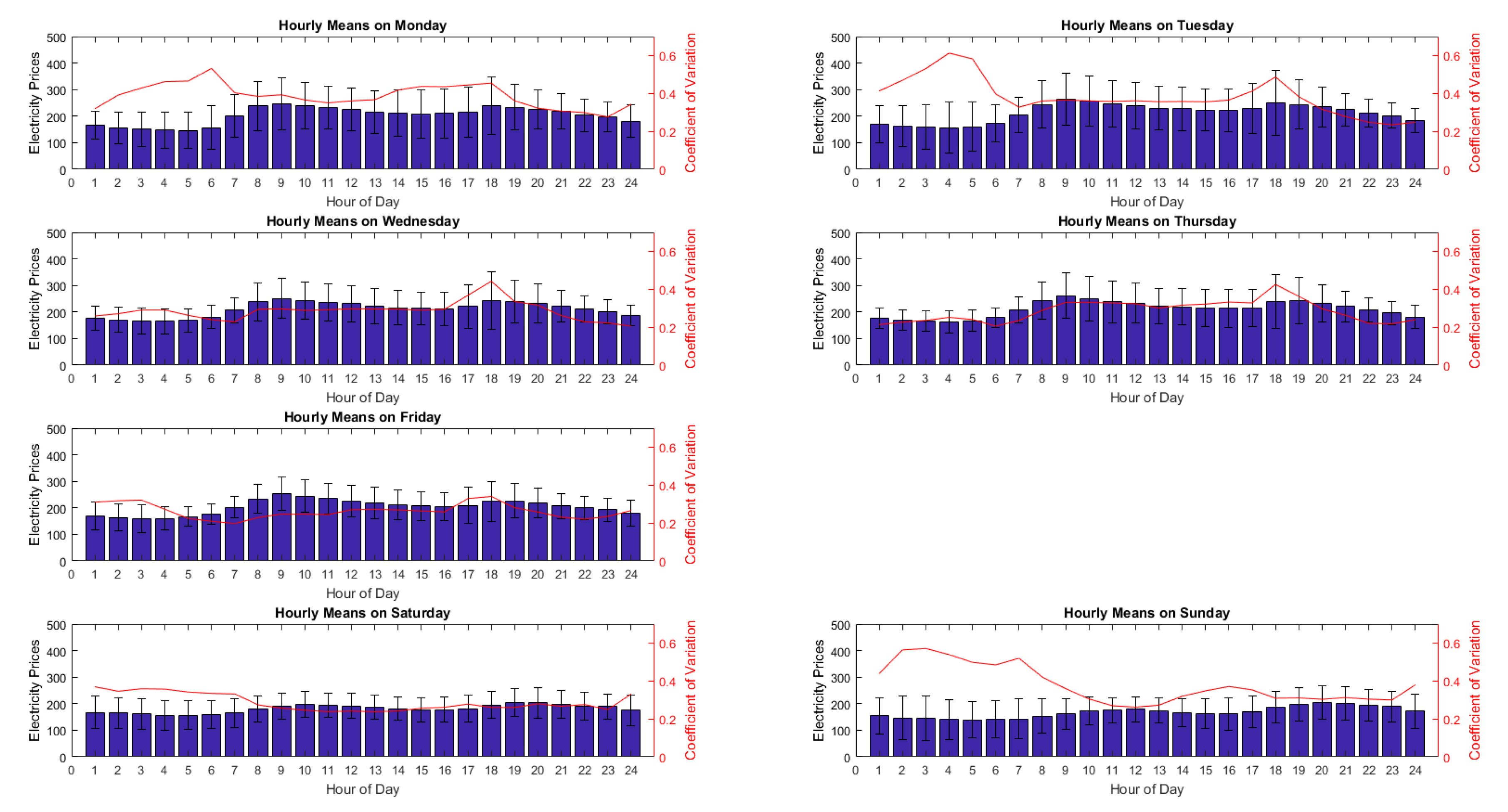
Figure 4 shows the hourly means for each weekday with the coefficient of variation, and the standard deviation bars. As expected from the data in Figure 3, Sundays and Saturdays have lower means. In each graph a wave with two local maximum can be identified. On weekdays the local maxima are at around 9 and 18, whereas on weekends they are shifted by almost 2 h and they are approximately at 11 and 20. On weekdays the first maxima is higher in contrast to the weekends. A daily seasonality is clearly observed from these figures.
Just by looking at the means at different intervals, different seasonality’s and different patterns of the data can be seen. Weekly and daily seasonalities are observed and this information should be properly included in the forecasting model, otherwise some information that should be carried in the forecasting model will be missing. Leaving out yearly seasonality in consideration of our data is a justifiable approach as our time span only covers more than a year and not decades.
3.1. Autocorrelation of the Time Series
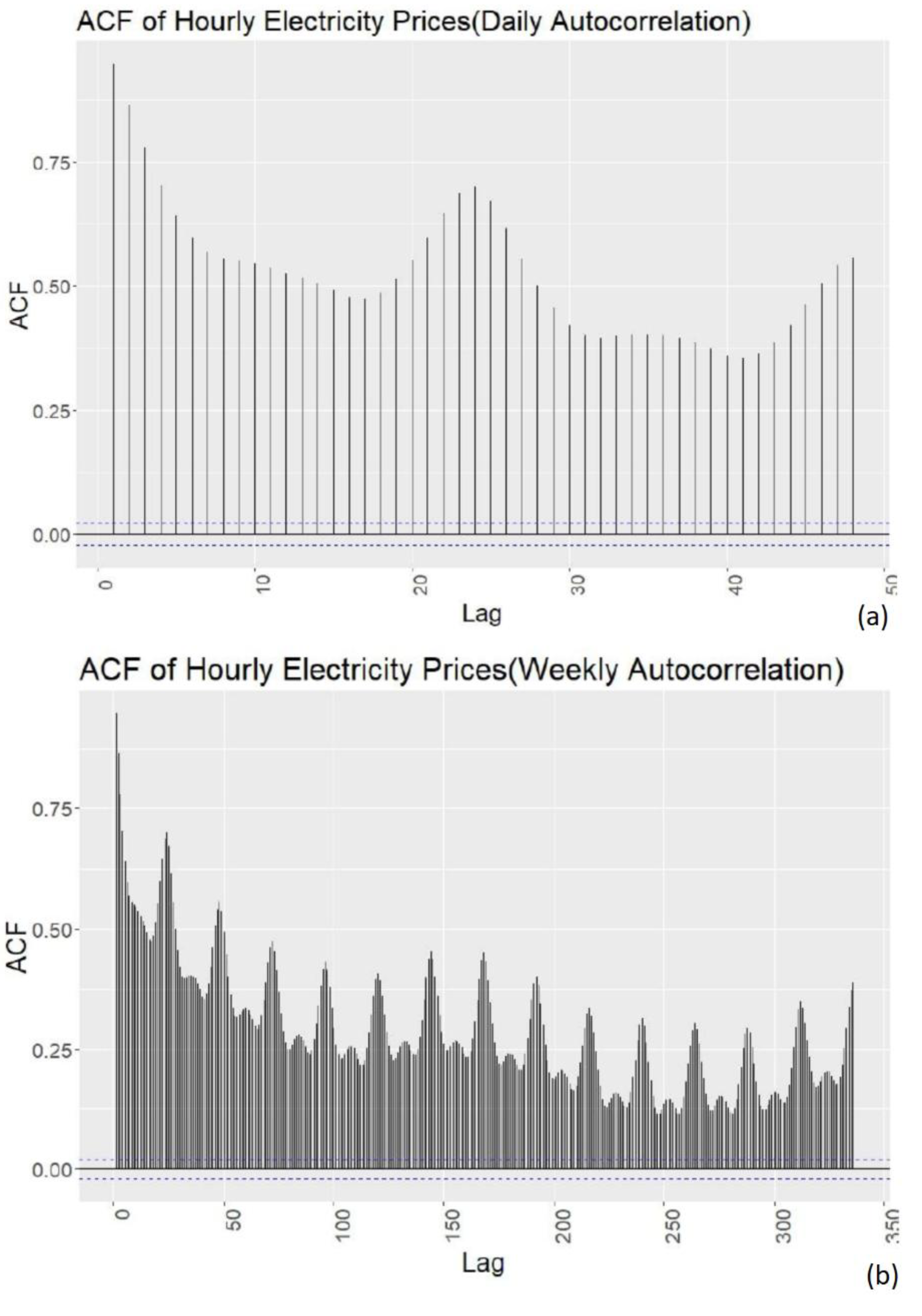
To further analyse the data and confirm the daily and weekly seasonality observed in previous section autocorrelations functions can be inspected. Autocorrelation is the correlation, the linear relationship, between the function and the delayed version of the function [17]. Autocorrelation Function (ACF) will be used in the next sections also to test if the forecasting model is a good fit, or to see if there is more information left in the data that should be included in the model.
Looking at Figure 5a the local maximum can be seen at lag 24 and 48, indicating a daily seasonality as expected. Figure 5b shows both the daily and weekly seasonality. In Figure 5b it can be seen that the maximum at both at multiples of 24 and an increasing pattern at multiples of 168 (7 × 24) which is the weekly period. It is not possible to see the yearly seasonality with ACF because a much longer time period of the data would be needed than 1 year to observe the effect, therefore it is not included.
3.2. Decomposition of the Data
There are many different ways of decomposing data such as the classical, seasonal decomposition of time series by Loess (STL), X11. The main idea behind the composition is to divide the data into their components, which are generally the trend, seasonal and remainder parts. When applying additive decomposition it is assumed that the data comprise of the sum of its components. Multiplicative decomposition on the other hand assumes that the data are a multiplication of its components and it is mostly used when the variation in the data increases or decreases along with time. The data that will be used for forecasting in this paper do not show a linear relationship in their variation with time so an additive decomposition model will be preferred.
If the data have Seasonal, Trend and Remainder components the mathematical formula can be formed as below, where yt is the main data, St is the seasonal component, Tt is the trend component and Rt is the remainder component [17]:
Trying to explain it in a simple way, the Trend component can be thought of as the general level of the data. In the classical decomposition which is the simplest method, it is calculated as a moving average. Seasonal component is the part that is dependent on time or calendar and its pattern is repeated. Daily, Weekly or Annual effects are seasonal where as a cyclical effect that is unrelated to the calendar or time is not part of the seasonal component. Remainder component is the error or random part that is not captured by the seasonal or trend components.
It is noticed that there are there seasonalities observed in our data, Daily, Weekly, and Yearly. An equation that explains our data can be mathematically expressed as below, where Dt is the Daily seasonality, Wt is the Weekly seasonality and Yt is the Yearly seasonality. The data are relatively of high frequency and the decomposition model should be able to handle this:
Models mentioned above such as classical, STL or X11 cannot handle multiple seasonalities and are designed for less frequent data sets such as quarterly or annually. TBATS model is able to handle multiple seasonalities as well as high frequency data [30]. The model will be discussed in more detail in the next sections of the paper.
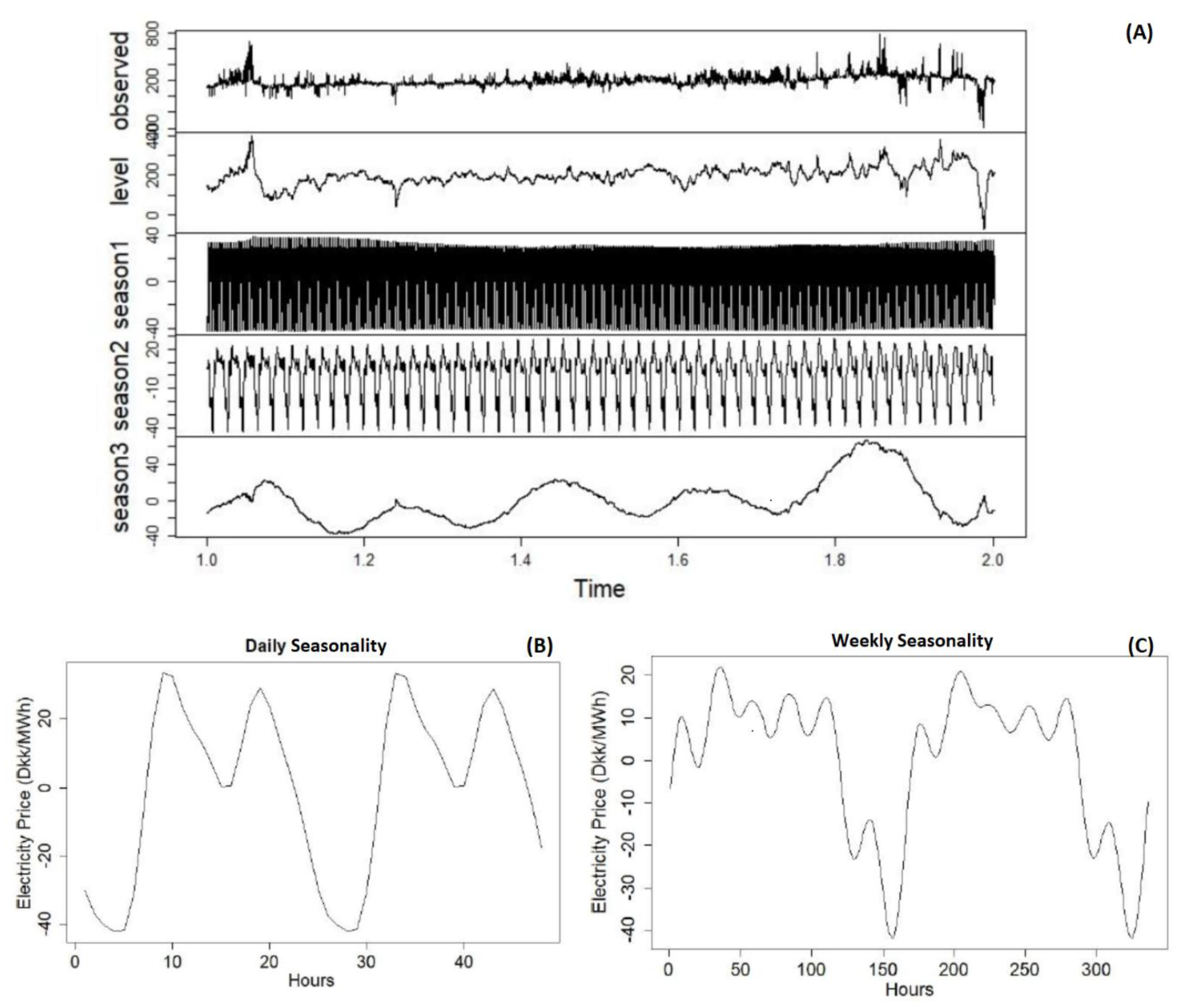
Figure 6A presents the application of TBATS decomposition. The first graph is the actual data, second is the level which is similar to trend, season1 is the daily seasonality, season2 is the weekly seasonality and season3 is the yearly seasonality. The decomposition and graph is generated by using R software, forecasting package [31], with “tbats()” function.
Looking closer at Figure 6B, which is a close up of season1 graph adjusted to include two days of data, daily seasonality can be observed. As expected, it is similar to hourly mean graph and it captures the construct with two local maximum points. It shows us that TBATS model has captured the daily seasonality to a satisfactory degree.
In Figure 6C, which is a close up of season2 graph including a two weeks span, weekly seasonality can be seen. As seen previously in the weekly mean graphs, weekdays are higher compared to the weekends. The data is adjusted to show Monday first, so that the lowest point seen around 150 corresponds to a Sunday. Similar to mean levels Sunday has the lowest value.
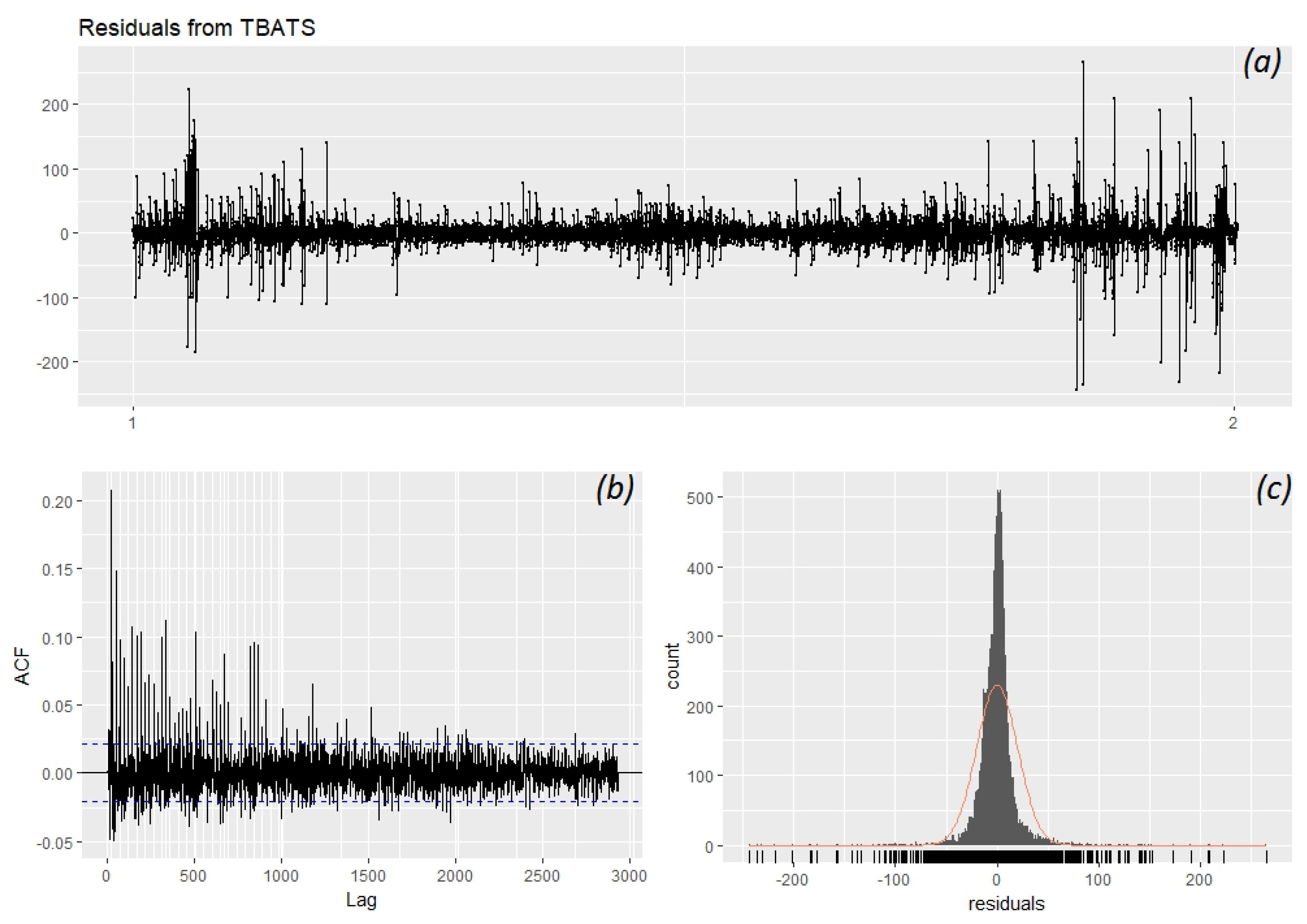
Upon closer inspection of season1 and season2 components it is seen that data seasonality seems to be captured in our model. One more thing to check is the residuals. If the information in the data is captured adequately, residuals should resemble white noise, meaning they should have 0 mean and it should be uncorrelated.
Inspecting Figure 6C and taking the mean of the residuals, it is seen that there is no bias and the mean is almost zero. The residuals follow a normal distribution however they are very high at some points and seem to have some correlation. Some explanations for this could be that the initial data have a lot of spikes, there are holiday effects that are not included in this model, and other external effects such as excess electricity production that leads to negative jumps due to high wind energy generation.
It is seen from Figure 7 that this model has satisfied our seasonality needs using high data frequency however, there are some things in the data that cannot be simply explained without referring to external factors. This shows that explanatory variables should be included in our model in order to capture the information in the data more accurately.
3.3. Explanatory Variables
Explanatory variables, sometimes also called as external regressors, are the external data that is used in the regression systems in order to get a better forecast. These regression systems carry the assumption that the forecast is a function of its past values (Autoregression) and a function of the external variables.
In this paper seven explanatory variables along with two dummy variables and a Fourier fit for seasonality is considered as external regressors. The seven explanatory variables, purposefully selected—explained in the following sections—are temperature, consumption prognosis, production prognosis, wind prognosis, oil prices, natural gas prices, and hydro reservoir levels. Two dummy variables are used to indicate weekends and holidays. Also the daily and weekly seasonality is fit through a Fourier function and fed into the ANN and ARIMA system as external regressors.
For the forecasting, future values of the explanatory variables are needed. In terms of this project it can be argued that temperature forecasts are highly accurate and available at various sources. Consumption, production and wind prognosis data are forecasts that are readily provided by Nordpool. Oil, natural gas and hydro levels are used with low frequency and they are not volatile so past values can be easily used. It should be noted that when evaluating forecasting errors, errors that might be in the explanatory variables are not included.
Table 1 shows the variables along with their correlation coefficients with the electricity prices. Actual contribution shows if the variable has contributed to the ARIMA and ANN models. For two variables knots are suggested however, they are not successful and knots should not be used. Out of the seven suggested variables only temperature has not contributed to the forecast and therefore it is better to omit it. The other variables should be included without any knots.
3.3.1. Temperature
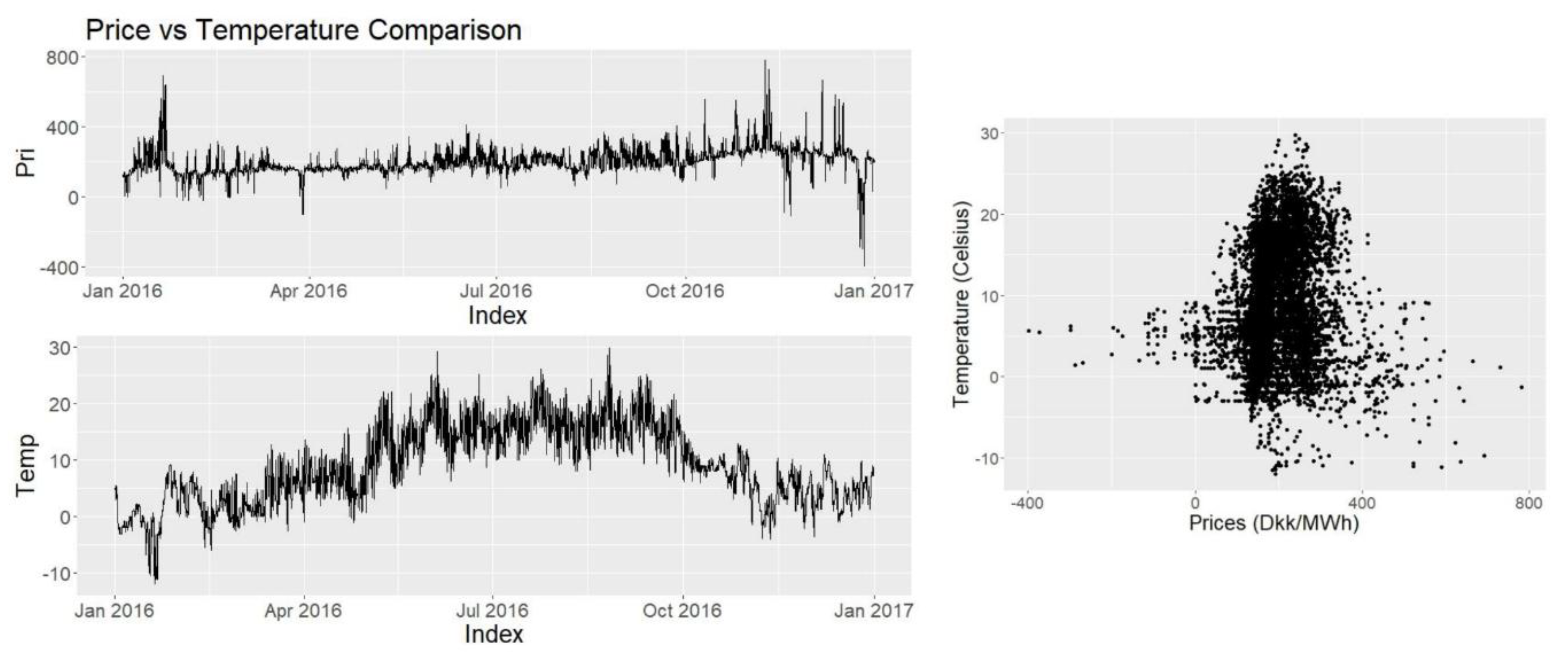
Temperature is included as an explanatory variable in the model for two main assumptions. First one is that in very cold or hot temperatures need for climate control creates additional consumption which may affect prices. Second is that temperature incorporates daily and annual cycles and it can be helpful in explaining other information such as wind which is directly related with the production.
Inspecting Figure 8 it is seen that the increase in temperature does not have any visible effect on prices, however when temperature falls below 0 in January a spike in the prices is observed. Also in October when the temperature is below 10 degrees, price levels have risen while is not the same case before April. Calculating the correlation coefficient we find that CPT = 0.0567. It seems insignificant however looking at Figure 8, which is a scatterplot, it is seen that prices below 0 degrees has a linear effect on prices. This is consistent with our previous comments and it suggests that temperature should be used as a variable with a knot at 0 degrees.
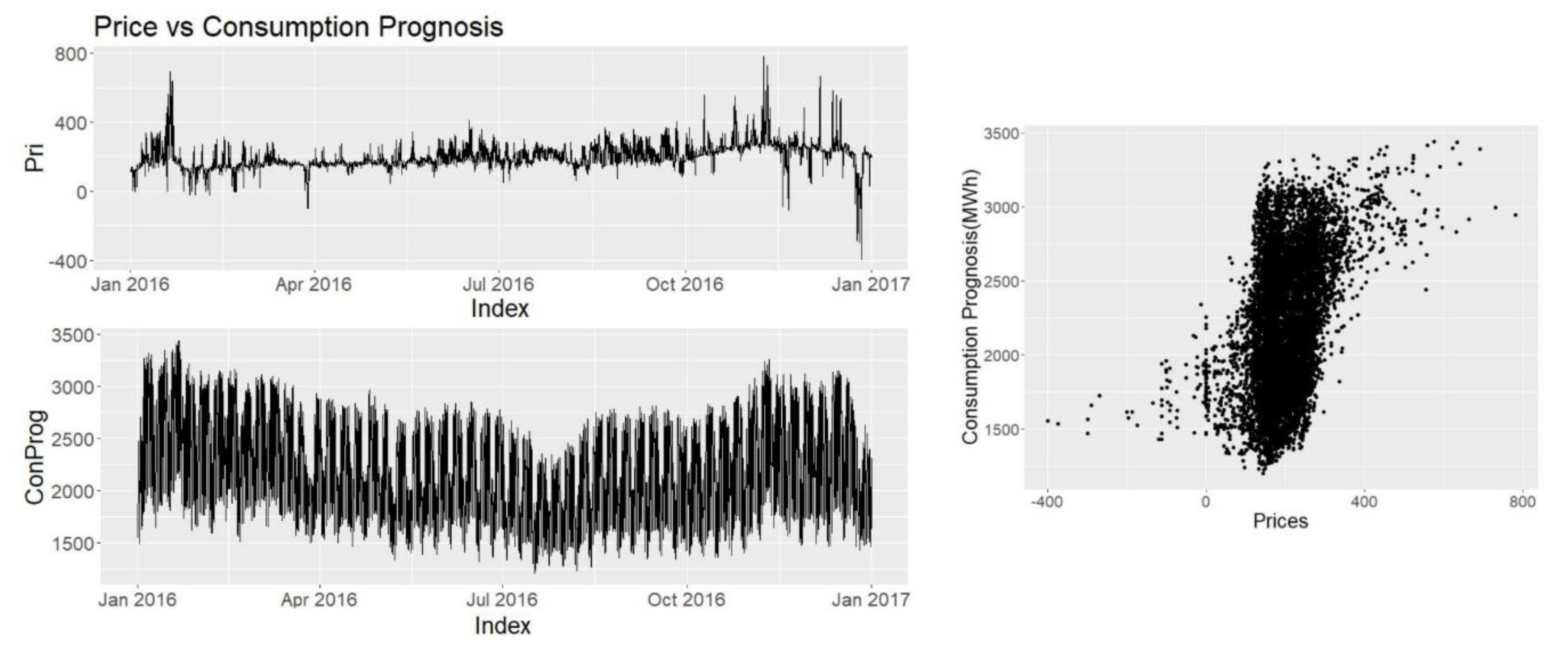
3.3.2. Consumption Prognosis
This data is presented in Nordpool website along with production and wind prognosis. It is assumed that it is directly related with prices as consumption of electricity is one of the uncontrolled variables in price formation.
It is seen (Figure 9) that consumption prognosis results in a spiky graph, probably capturing daily, weekly cycles along with the holiday effects. At the end of December, it can be observed that the decrease of consumption prognosis is related to the price decrease. Looking at the scatterplot in Figure 9 it can be observed that consumption has a positive correlation with the price and it is most noticeable at the extremes. Correlation coefficient is CPCP = 0.43, which is significant and much higher than temperature.
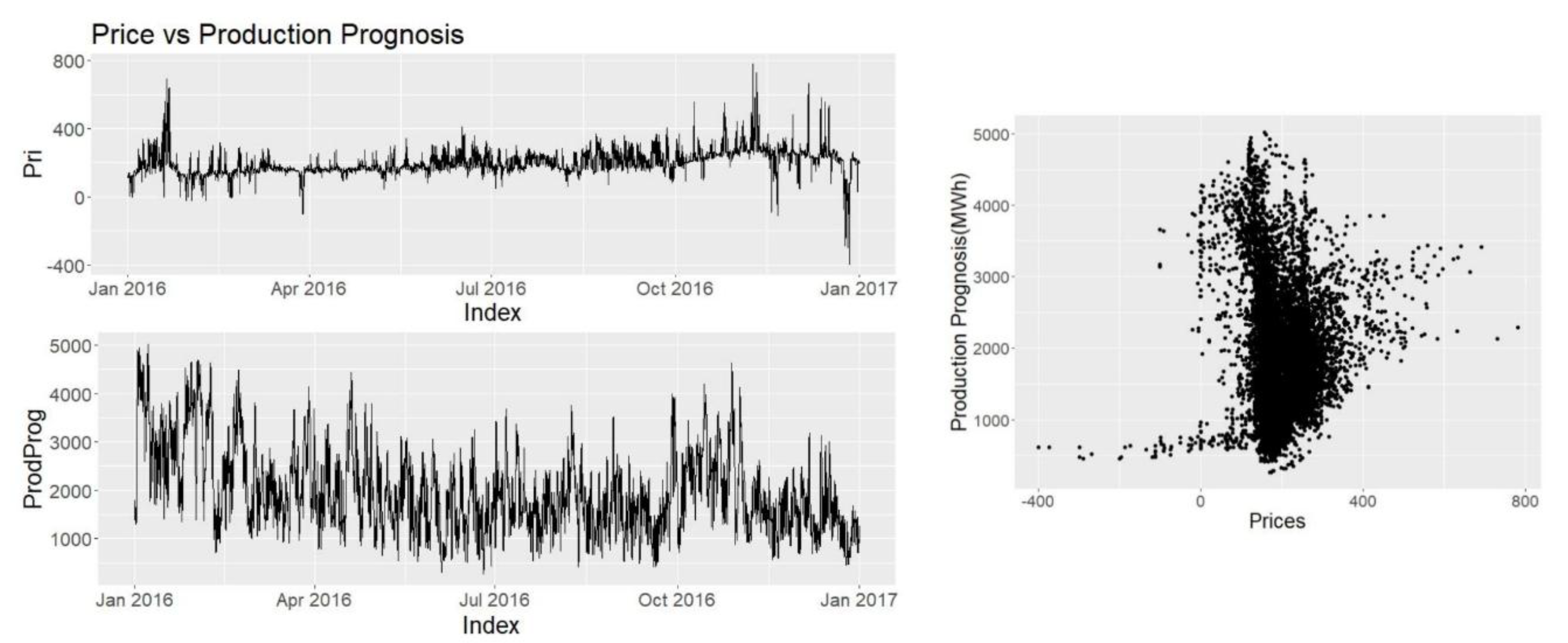
3.3.3. Production Prognosis
Electricity price formation can be seen as some function of consumption and production however consumption is an uncontrolled variable whereas production is controlled except solar and wind power. No apparent pattern catches the eye in Figure 10. Correlation coefficient is CPPP = −0.0448, it is even lower than temperature. Inspecting the scatterplot the only meaningful pattern is seen when production prognosis is below 1000 MWh, where very low prices can be observed. Production is actually driven by the consumption and prices and not the other way around, however this data might be more useful with a knot at 1000 MWh.
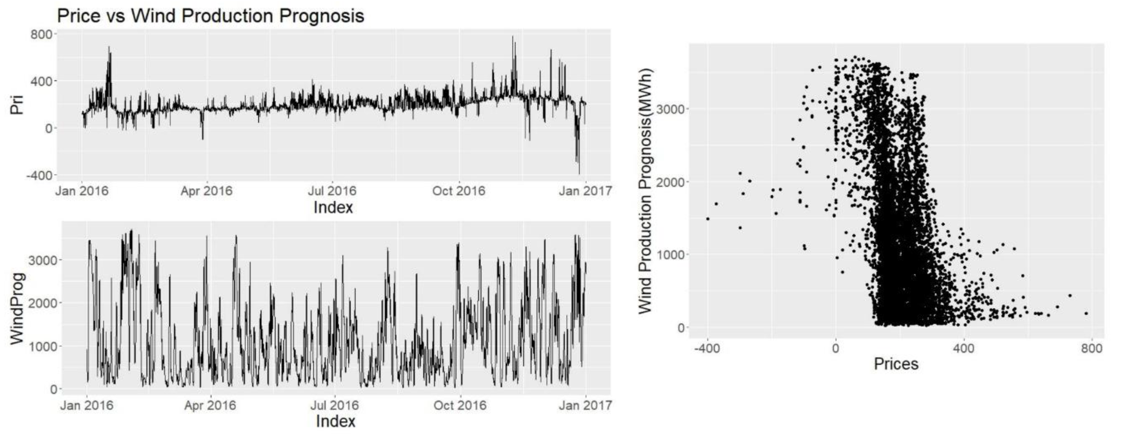
3.3.4. Wind Production Prognosis
Looking at Figure 11 two patterns catch the eye, where in January there is a sharp fall in wind production prognosis and a sharp increase in prices and the opposite happening at the end of December. Correlation coefficient is CPWP = −0.368 which is almost 8 times of production prognosis. Wind is very important for Denmark due to high penetration rate.
In the scatterplot at Figure 11 it is seen that high prices only happen when there is very little wind and a lower price level is very likely as the wind production is increased.
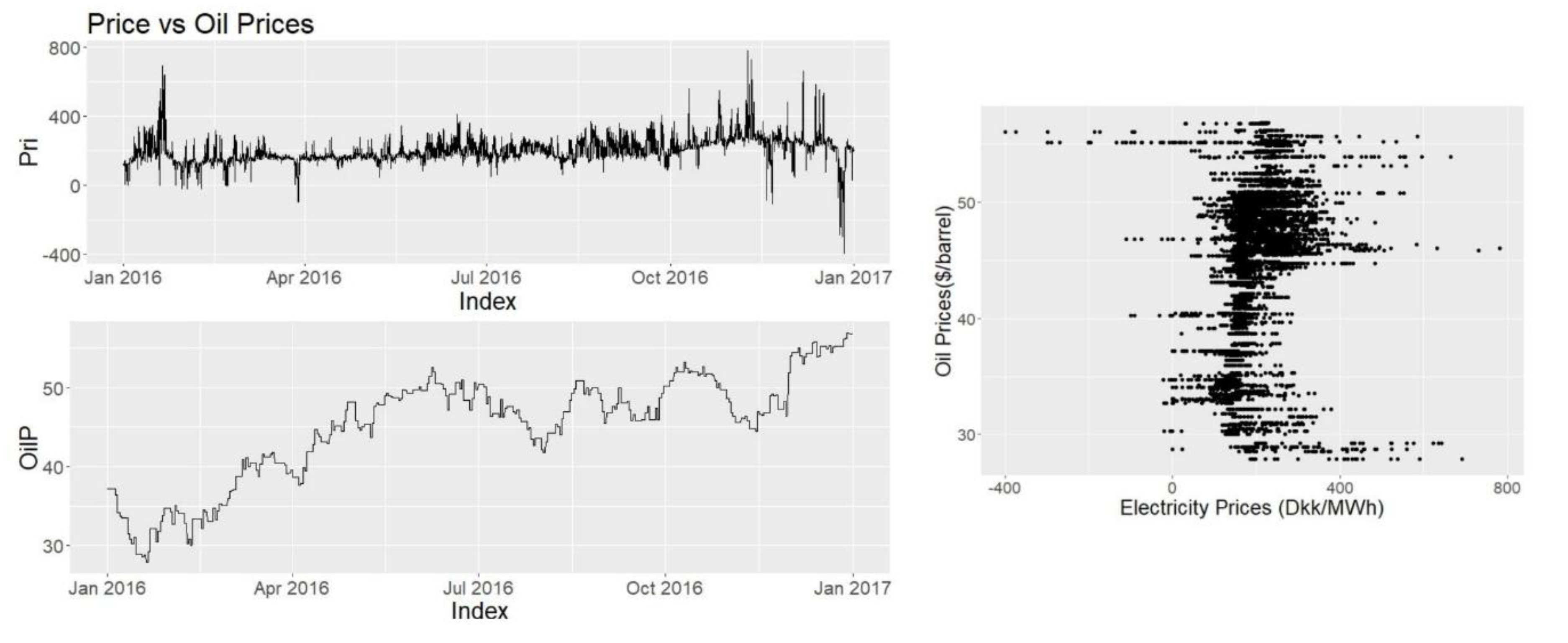
3.3.5. Oil Prices
Oil has provided the 37% of the gross energy consumption of Denmark in 2016 therefore, it is assumed that the oil prices have some importance in term of electricity prices. By checking Figure 12 it is not possible to see a price level increase with the increase of oil prices therefore a low correlation is expected. Neither of the scatterplots show a strong correlation and since low consumption during Christmas time coincided with high oil prices, the oil prices do not seem like a major price driver at their current change rate. When calculated the correlation was found to be 0.259.
3.3.6. Natural Gas Prices
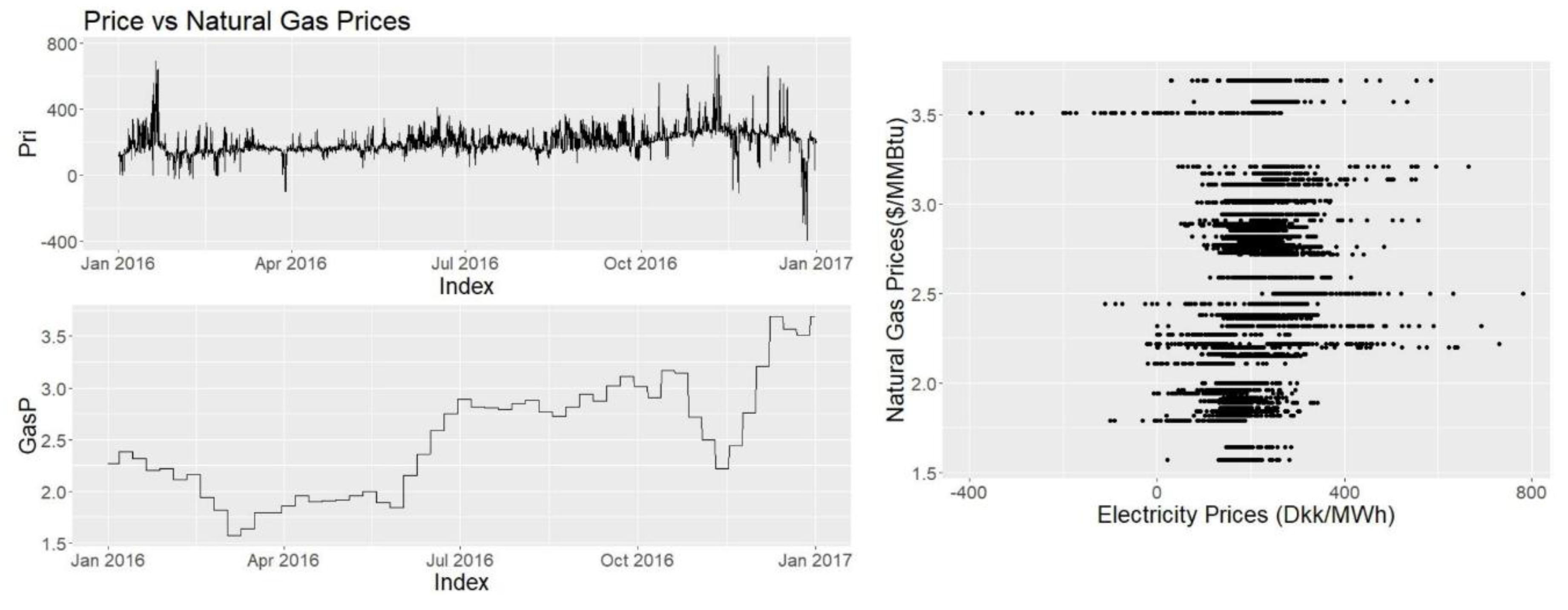
In 2016, 16% of the gross energy consumption of Denmark has been provided by natural gas thus it is assumed that natural gas prices have some significance over electricity prices. Natural gas price diagrams (Figure 13) look similar to oil price diagrams. The correlation coefficient is found to be 0.293. As the data frequency is lower for natural gas the graphs look discrete.
3.3.7. Hydro Reservoir Level
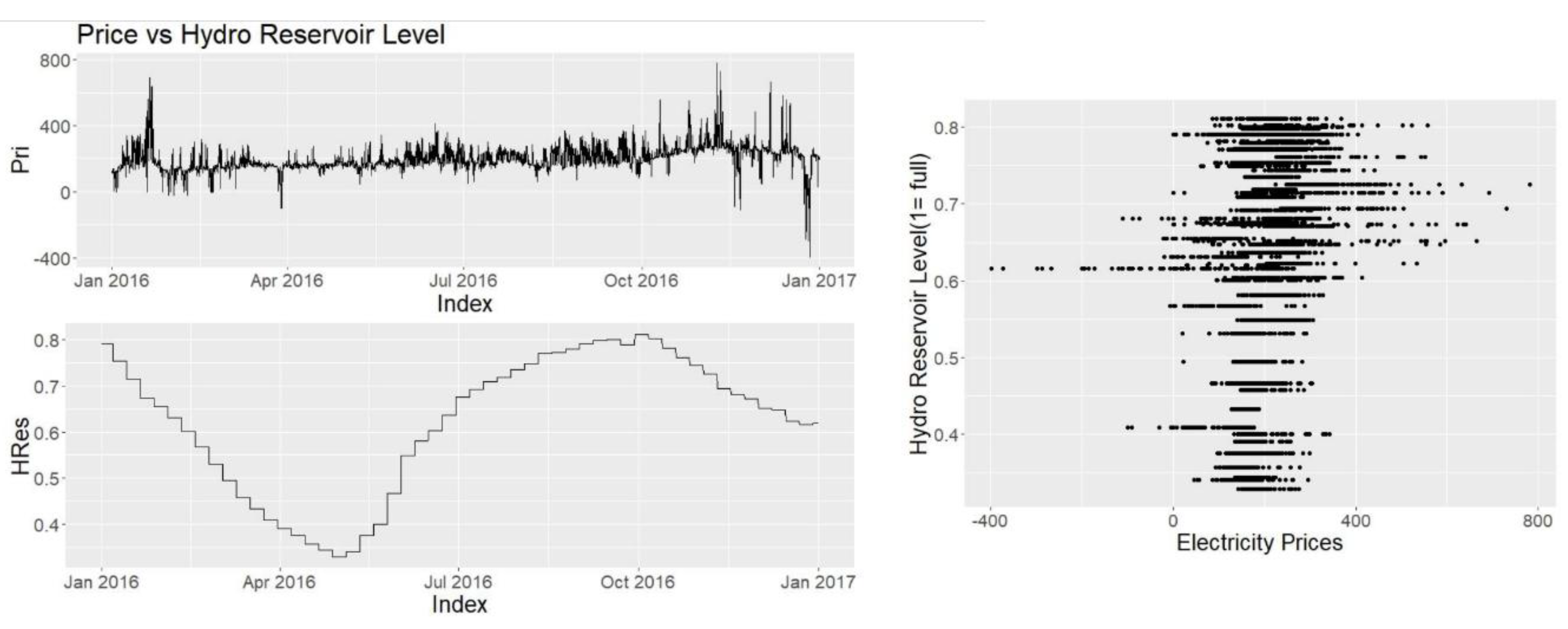
Hydro reservoir level is assumed to be important because it is a common way of storing the excess energy. For example if the electricity prices are negative in Denmark due to excess wind, Norway can purchase the electricity to pump water to their hydro reservoir level. This effect will be more visible when the hydro levels are empty than they were full. The data frequency for hydro reservoir level is taken as weekly, therefore the graph looks somewhat discrete (Figure 14). The correlation coefficient is found to be C = 0.313. The coefficient is higher than oil and natural gas.
4. Forecasts and Results
The outcome of the project is the artifact which is the software that is used for the forecasting also the point forecasts generated for the forecasted time period. In this section point forecasts along with the actual values will be shared on graphics.
The graph regarding the whole forecasting period, 212 days, will be shared. Then six weekly graphs will be presented, beginning with the 2 January with five week intervals to dismiss any monthly bias. As the weekly graphs will be “zoomed” they will reveal an indication of the actual performance of the models.
One important thing to discuss before getting to the forecasts is that the comparison for the actual prices in 2016 and 2017. This is particularly important as 2016 data is used for training, the forecasts will try to imitate the training set and carry their characteristics. If there is a significant difference between the training set and the test set, then a higher error in the forecasts can be expected.
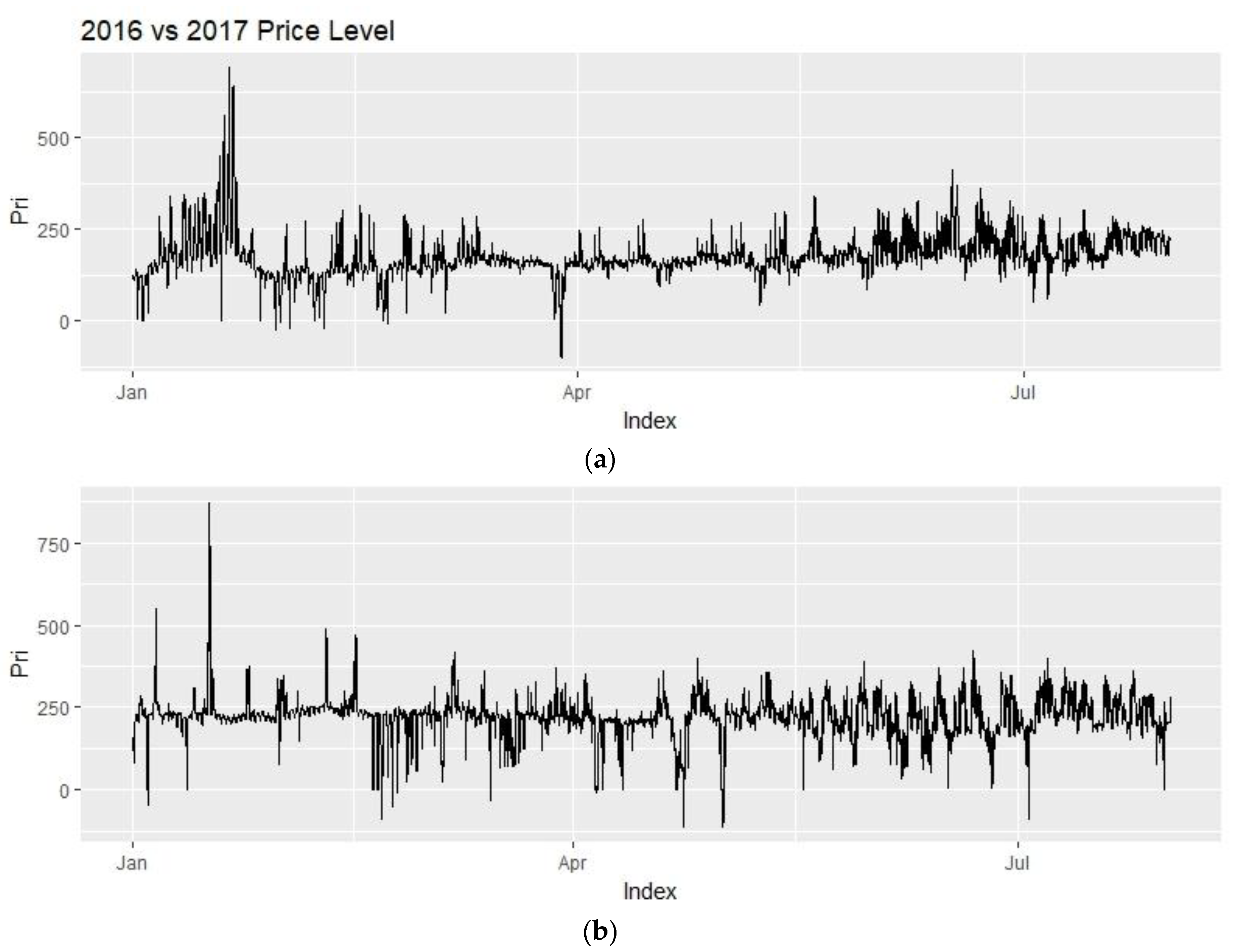
In Figure 15, the top graph shows the electricity prices for the year 2016 and below graph shows the prices for year 2017. The data sets are limited to the forecasting interval for the ease of comparison.
The mean price level has increased around 25% from comparing 2016 to 2017 (Table 2). The standard deviation increased around 11%.
Looking at Figure 15, prices in January 2016 are very volatile and above average, and after April they are pretty much at the same level of volatility. In 2017, the volatility is higher and seems to spread more evenly throughout the year.
4.1. TBATS
Unlike many other models that are widely used, Trigonometric Exponential Smoothing State Space model with Box-Cox transformation, ARMA errors, Trend and Seasonal Components (TBATS) is forecasting model that allows multiple, complex and dynamic seasonalities in time series. TBATS uses trigonometric approach for decomposing the seasonalities which allows for forecasting of much frequent seasonalties such as daily seasonality. The model also uses maximum likelihood estimation by least squares method, therefore a need for ad-hoc initial parameters is diminished. In addition, the method reduces the computational load [32,33]. One assumption using the model is that the error distribution fits the Gaussian distribution, which is applicable when the level of the data is sufficiently distant from the origin [34]. One disadvantage of the TBATS model is that it does not allow for any use with external regressors.
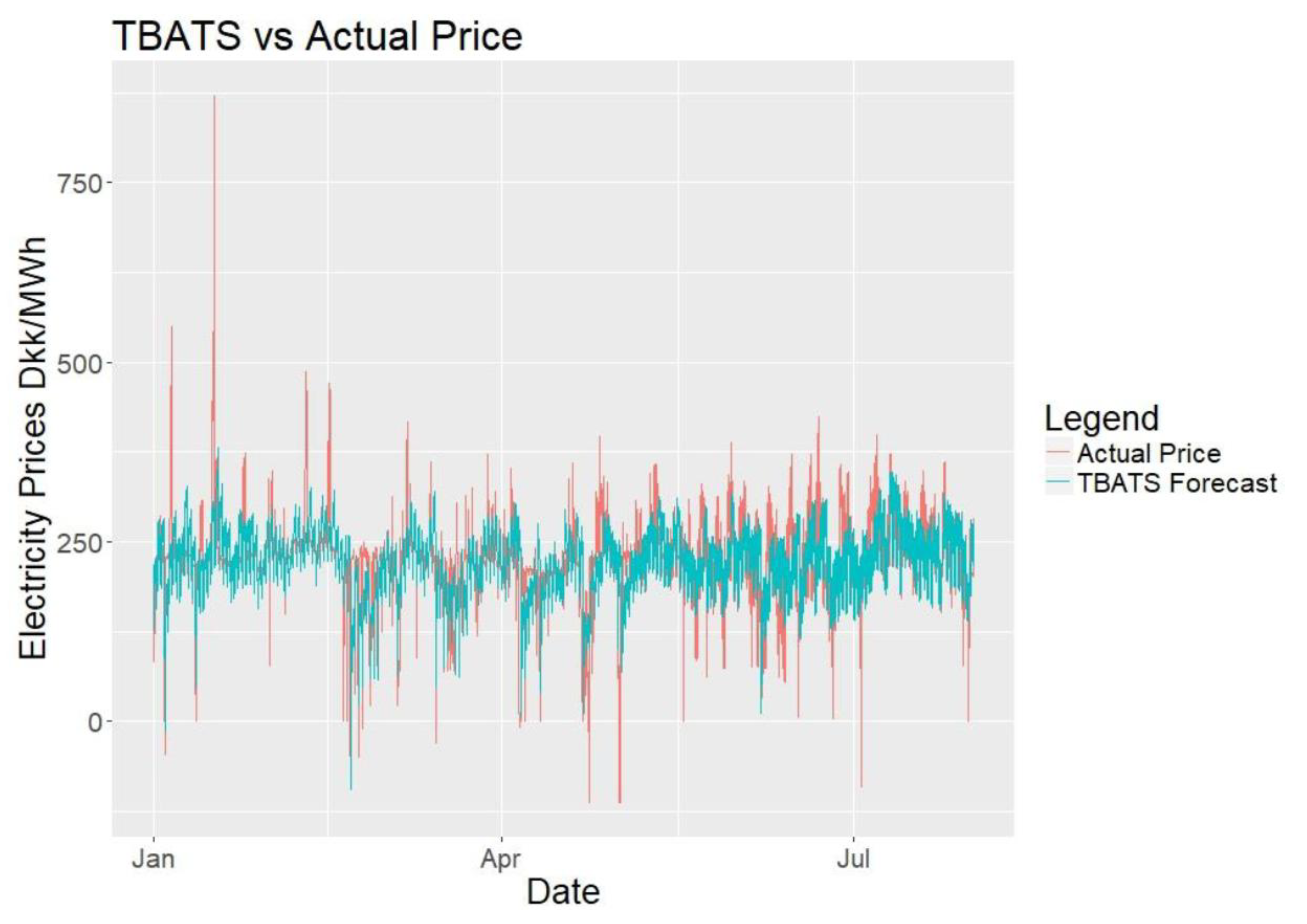
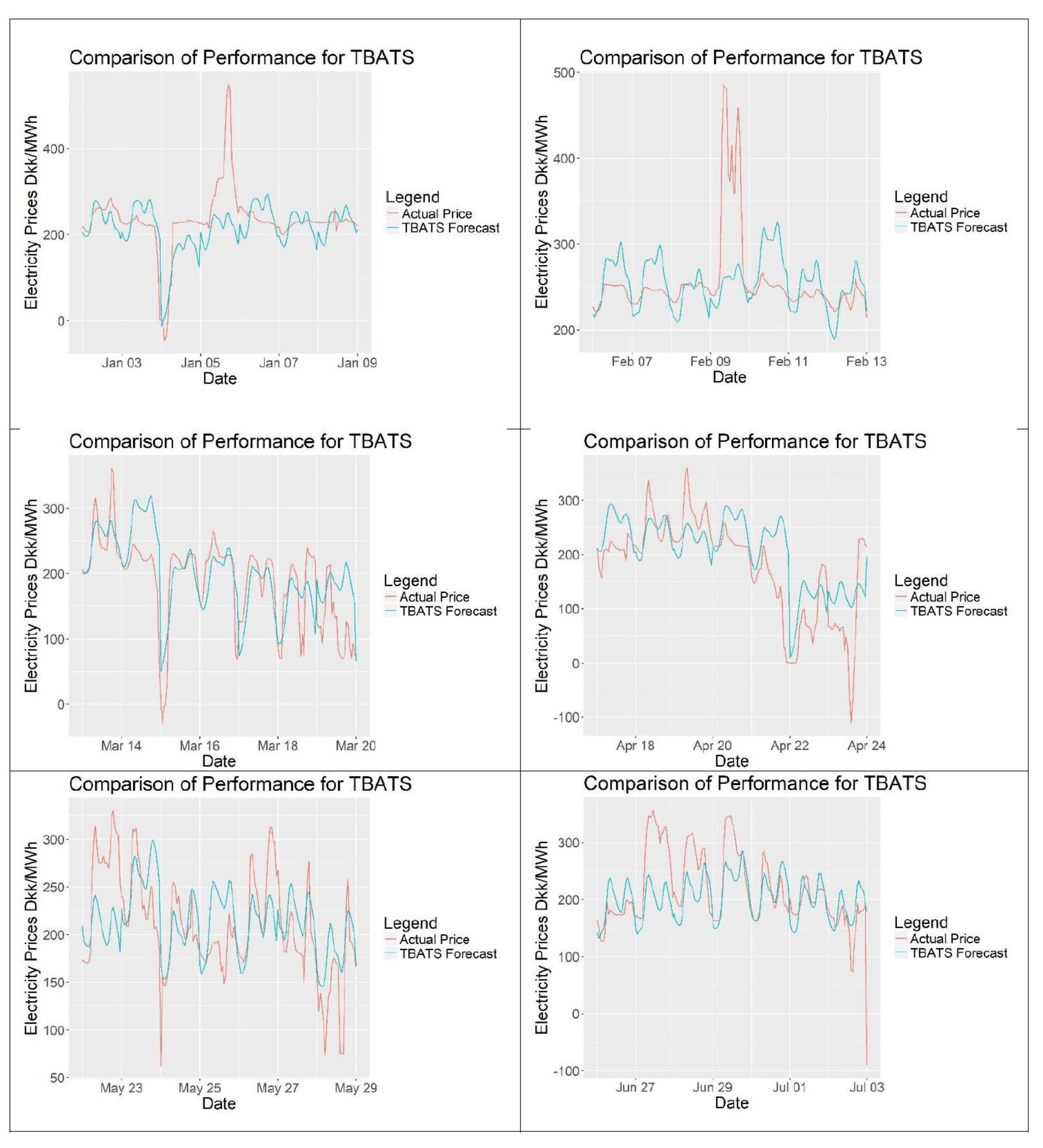
Figure 16 shows the TBATS forecasts against actual data for the complete forecasting period. Figure 17 shows close-up sections of six different weekly periods, which clearly shows the daily decomposition pattern seen in decomposition section. Although the model looks repetitive, it seems to fit the data to a satisfactory degree. At some points, it is seen that TBATS forecast cannot follow the spikes of the data.
4.2. Non-Seasonal ARIMA with External Regressors
Autoregressive integrated moving average (ARIMA) is one of the most used forecasting methods along with exponential smoothing [28]. Autoregression is feeding the past data values as inputs in order to predict the future values. A non-seasonal ARIMA model is a combination of Autoregression and a moving average. ARIMA models can also be used with external regressors which is an advantage over TBATS. Seasonal ARIMA models are not considered in our forecasts as they only support single seasonality.
In order to capture the seasonality effects in our data, a fit for the seasonalities with Fourier series will be used [35] and then this data will be fed together with other regressors. “fourier()” function from forecasting package is utilized in order to fit the seasonalities using a Fourier function. “auto.arima()” function from the same package is used to make the actual fit along with using additional command seasonal = FALSE [36].
“auto.arima()” function is an automated algorithm that is used in order to choose the best coefficients in an ARIMA model and it is a variation of Hyndman and Khandakar [28] algorithm. It uses unit root tests, and minimization of AIC and MLE to get to the result. AIC as a measure of goodness of fit. AIC is preferred over other methods as it penalizes complexity while evaluating the goodness of fit [17].
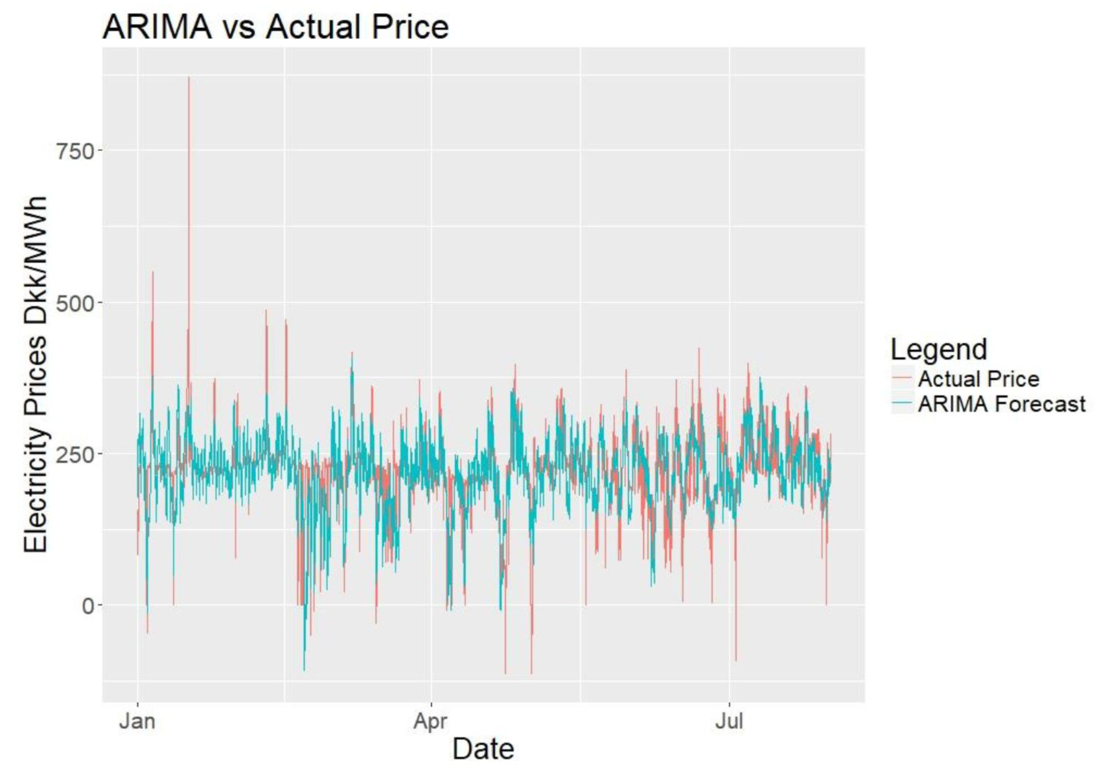
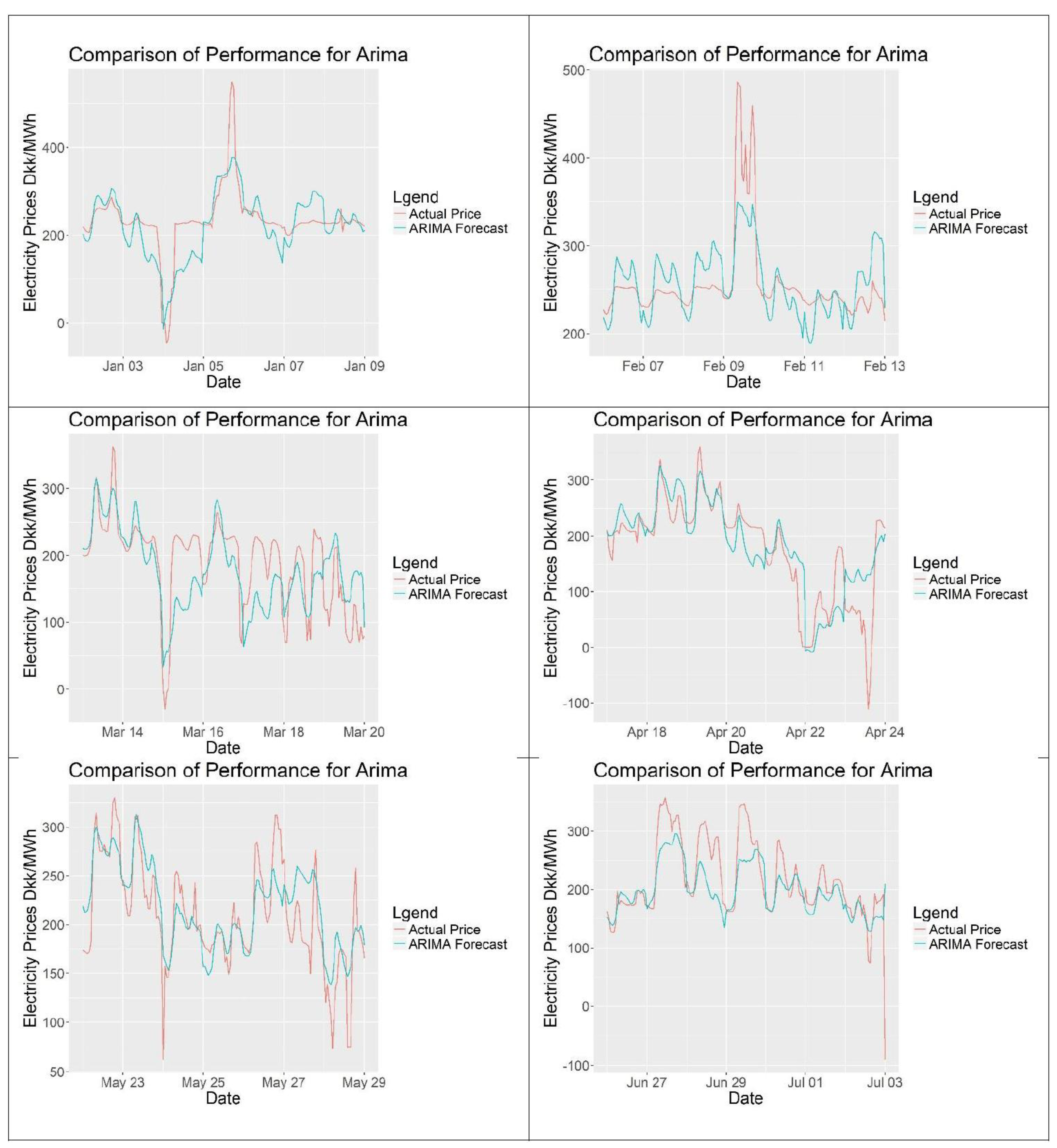
Figure 18 shows the ARIMA forecasts against actual data for the complete forecasting period. Figure 19 shows close-up sections of 6 different weekly periods. The model looks less repetitive than TBATS with the daily cycles being harder to identify. The forecasts follow the trend and seem to fit the data well.
4.3. Artificial Neural Network-Nnetar
Artificial Neural Networks (ANN) are a subgroup of machine learning systems which are computational systems with a design mimicking the biological neural networks. Just like the regression models they are fed with the training data and depending on the learning algorithm the ANN adjusts the outputs without any pre-assumptions. The advantage of ANN’s is that they can adapt to complex nonlinear systems and they can be used with external regressors [31,32,33,34,35]. A large number of data is beneficial for an accurate forecasting performance from ANN’s and this is suitable as the training data sample used in this paper is quite large [36].
Similar to ARIMA models in the application, Fourier modelled seasonalities are used as external regressors. “nnetar()” function under forecasting package is utilized to make a fit using an autoregressive ANN. The used network structure contains a feed forward neural network with a single hidden layer and the activation function is a nonlinear logistic function [33,36].
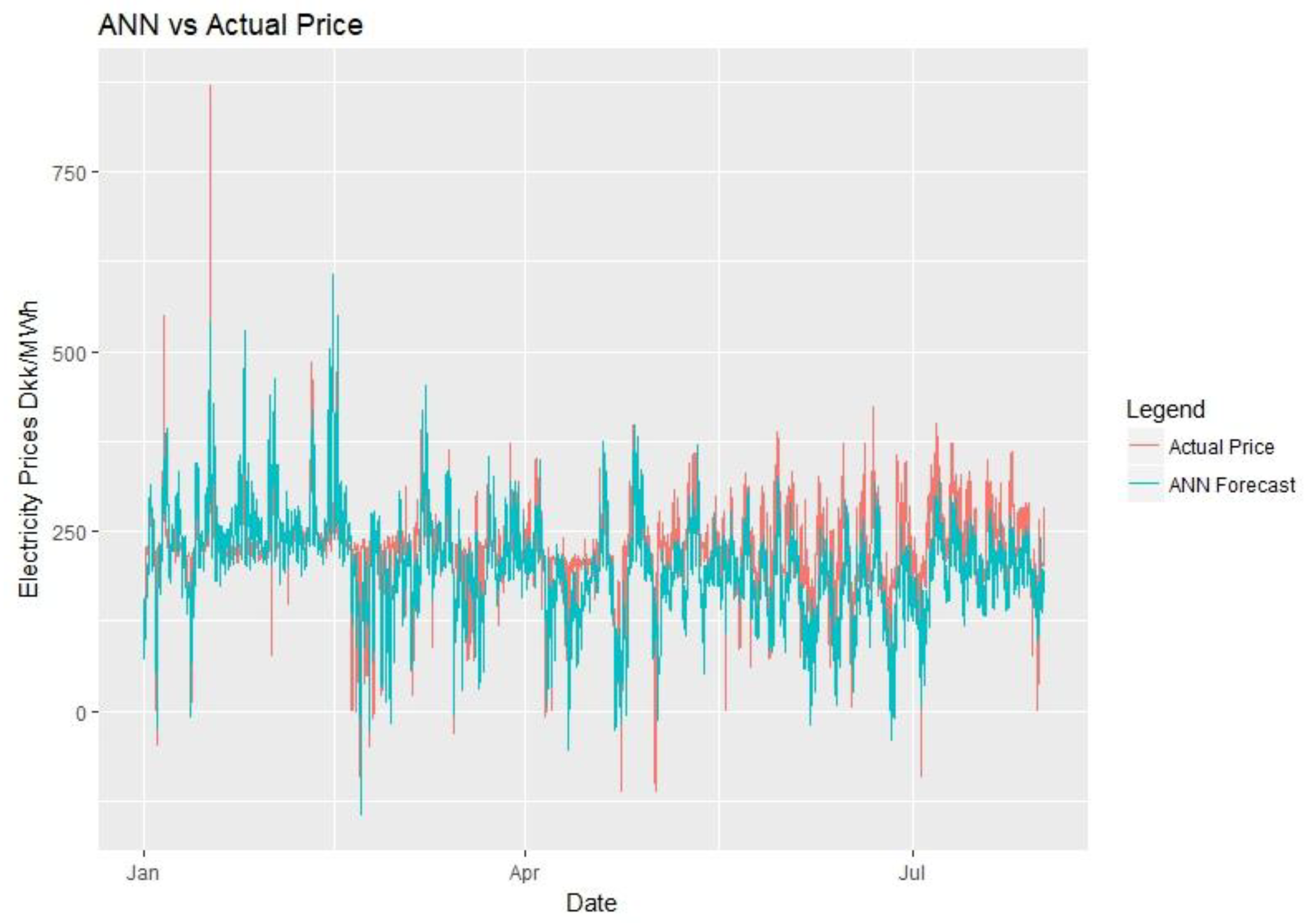
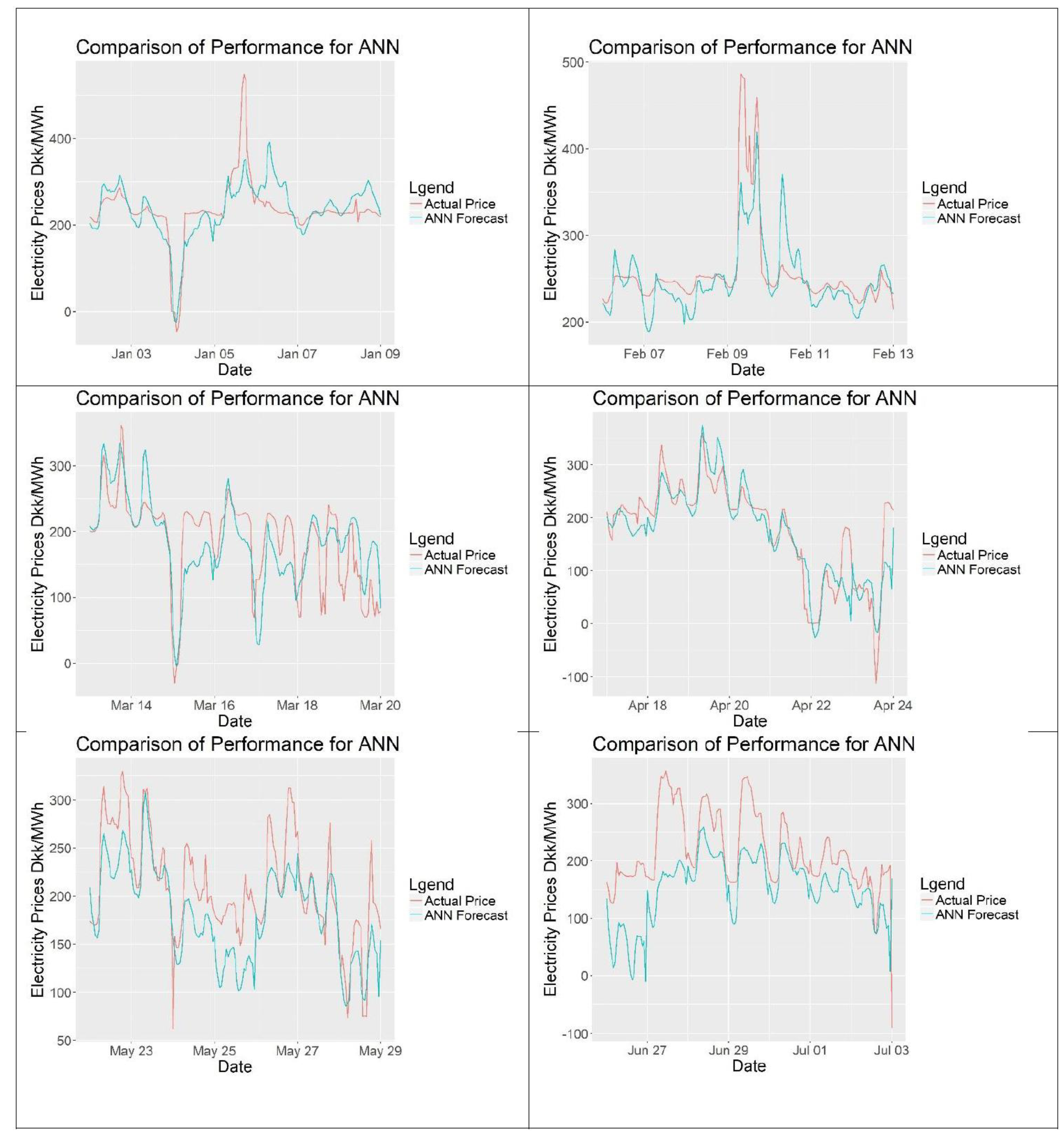
Figure 20 shows the ANN forecasts against actual data for the complete forecasting period. Figure 21 shows close-up sections of six different weekly periods. The model looks spikier than others do and it still contains the daily seasonality. The forecasts follow the trend and seem to fit the data well.
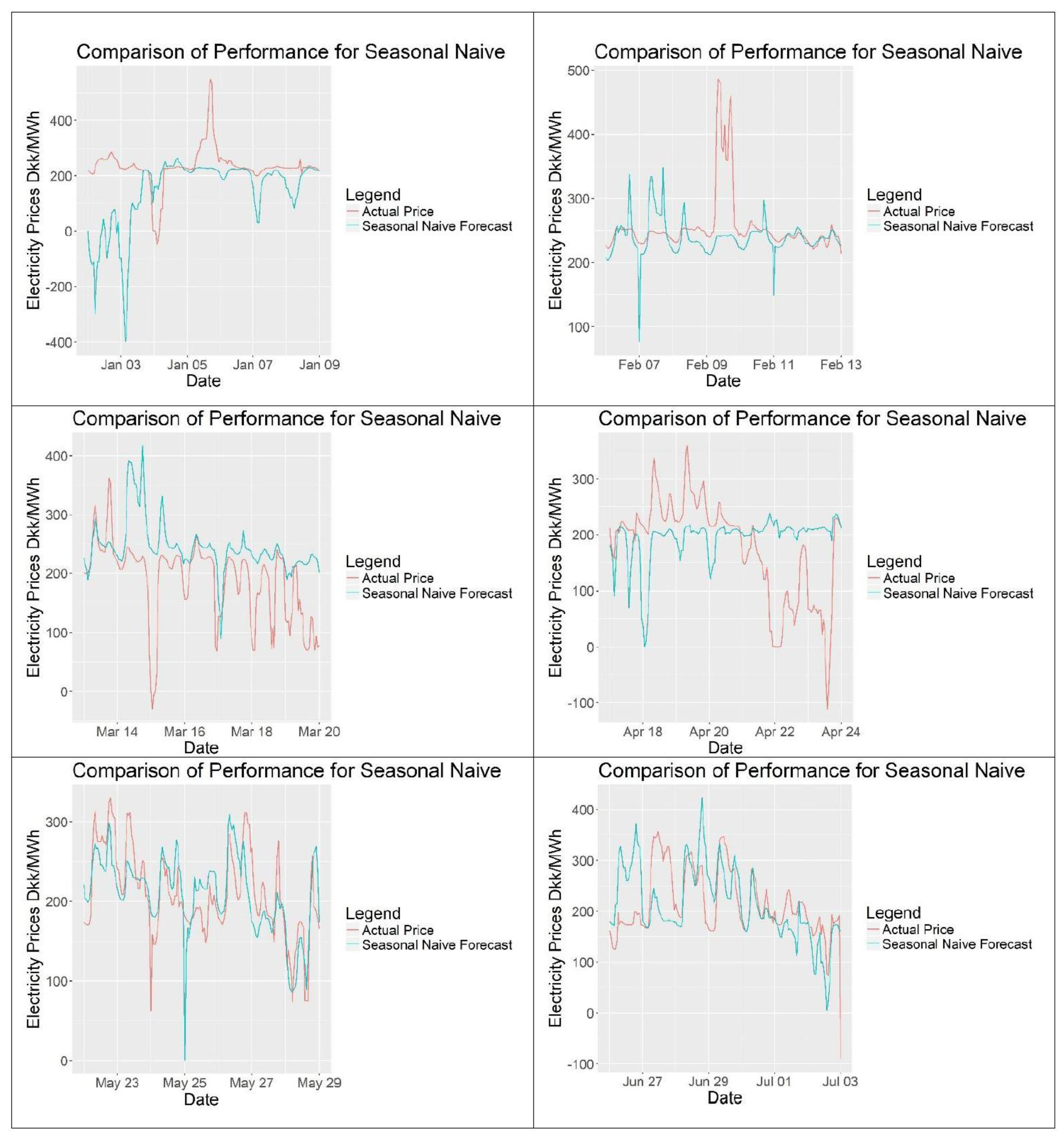
4.4. Seasonal Naïve (Benchmark)
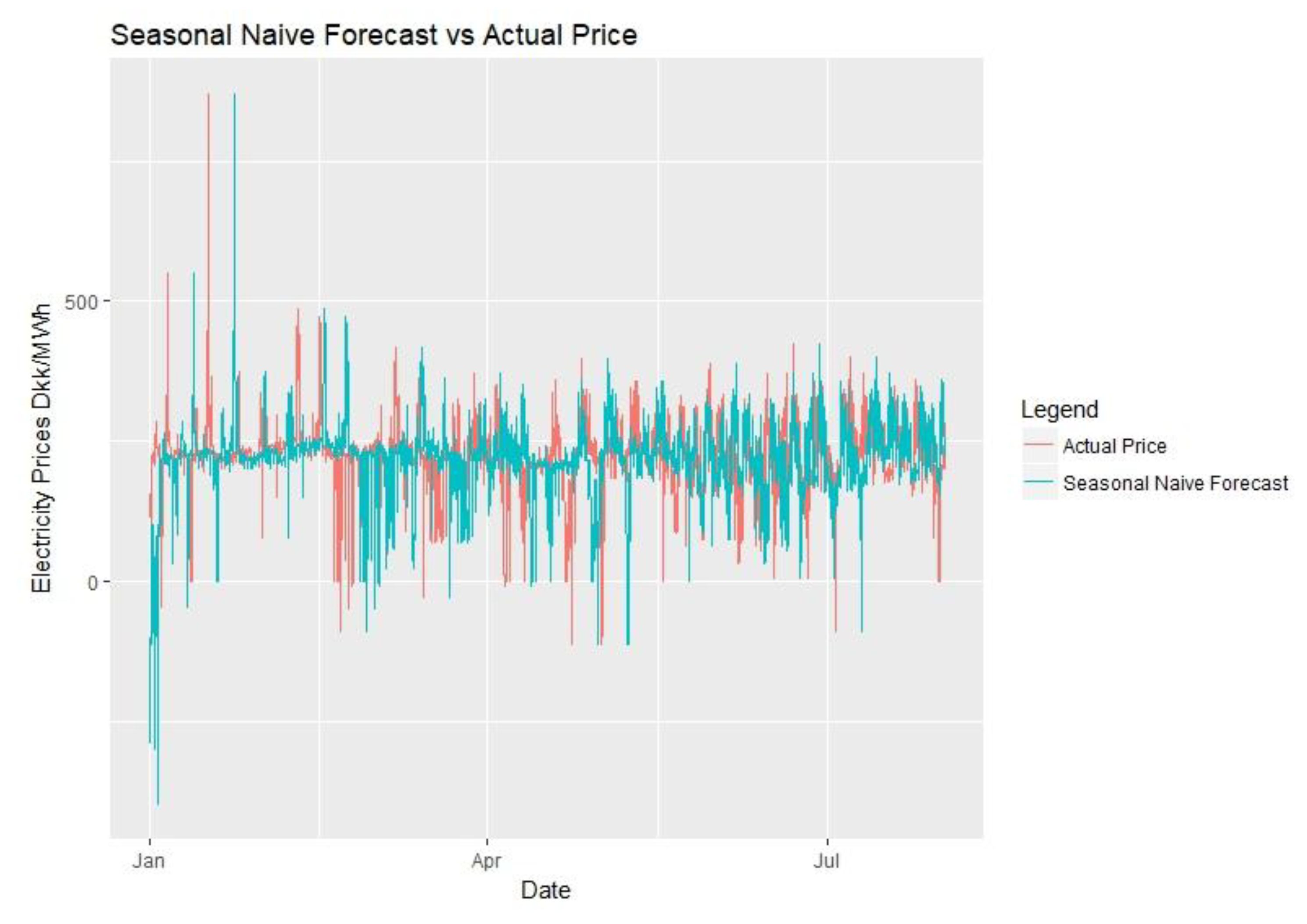
Naïve method in forecasting is simply assuming that the next forecast is equal to the previous available data. Seasonal naïve is a variation where the forecast is equal to the data from the last season, for example, a seasonal naïve forecast for the electricity price of this Sunday assumes that it is equal to the previous Sunday. This method can be further enhanced with the adoption of a drift coefficient if the level of the data is increasing or decreasing [17].
In this research paper, seasonal naïve method is used as a benchmark, meaning if the other tested models are performing worse than the seasonal naïve method it is possible to conclude that they are not working properly. As the implemented models are more complicated it is expected that they outperform the seasonal naïve.
4.5. Evaluation and Comparison of Forecasts
In the evaluation of the forecast, approximately seven months of forecast is used, more specifically 212 days and 5088-point forecasts were considered starting with 1 January 2017 in all forecasting models.
For the evaluation of forecasting performance, different error indications can be defined and used. As electricity prices include positive, negative and zero values using percentage errors do not yield meaningful results. More specifically percentage errors result infinity when the actual data is 0. Instead of percentage errors, scale-dependent or scaled errors may be used.
In this paper, error will be indicated in two forms, as root mean squared error (RMSE) and as mean absolute error (MAE). A forecast that focuses on minimizing MAE will yield forecasts of median whereas minimizing RMSE will yield forecasts of mean [7,33]. Using an expanding forecast for 7 months 212 forecasts are generated with 24 data points in each one. In calculation of the accuracy, this yields us 212 error values calculated as seen below. In Table 3, the values shown are the mean, minimum, maximum and standard deviation of these 212 accuracy values.
Formulas for calculating RMSE and MAE can be found below. In the formulas T is the forecasting span, Ph is the actual value and is the forecasted value. In our calculations “accuracy()” function from the forecast package is utilized. This function calculates the mean error, MAE, mean absolute percentage error, mean absolute seasonal error, mean percentage error and RMSE automatically. Then the mean minimum and maximum values of the related errors were taken, to reach to the values at Table 3:
From Table 3 and the mean values it is seen that all the models have outperformed the seasonal naïve benchmark significantly. It is also inspected that best forecasts are achieved with Non-Seasonal ARIMA model. It is interesting to see that ANN-nnetar was outperformed by TBATS as ANN uses external regressors. It is intuitive to assume ANN would outperform a method that doesn’t use any regressors. This shows that nnetar might not be suitable for this kind of forecasting and a more complex ANN model should be more beneficial in terms of forecasting performance. On the other hand, nnetar model has the lowest maximum error and depending on the error function it might be a preferred model. ANN model could be more useful in a setting where he cost of an error increases exponentially as we get further away from the actual value. In addition, it can be speculated that as the amount of data used gets bigger ANN model could yield better mean values. Further to these low maximum errors might suggest that it is adapting faster to errors than other models and it could be more successful over spiky periods.
4.6. Backwards Feature Elimination
Backwards feature elimination is a variable reduction method that is used to minimize the number of external regressors, optimize the computation time and minimize the error. Assuming there are n = 7 regressors (excluding Fourier seasonalities and dummies) the ARIMA forecast will be run with n − 1 = 6 regressors and each time a different regressor will be eliminated from the forecast and the error will be evaluated. This will allow us to see if there are any variables that are unnecessary, disruptive or that are extremely important for better forecasts [37]. Benchmark for comparison will be the Non-Seasonal ARIMA with all seven regressors (Table 4).
Looking at the error results for elimination the only one better than the benchmark is actually the temperature variable. There is 1.6% improvement in the mean error for RMSE and 3.85% improvement in mean MAE error. There is significant improvement in both RMSE and MAE maximum error respectively 28.8% and 43.4%. Improvement in standard deviation is also significant and it is 23.2% in RMSE and 27.4% in MAE.
This shows us that the variables chosen actually contribute to the regression model except for the temperature. As discussed, temperature has a low correlation but inspecting the scatterplot it was argued that a knot at 0 degree might be useful. Before removing the variable completely, implementing a knot could prove useful.
By making the following assumption, upon exclusion, the variable that results in the greatest increase in error has greater contribution to forecasts, it can be inferred which variable that has the greater importance. In terms of the different variables inspecting the mean error values, it is seen that consumption prognosis has the greatest positive effect on the forecasts. Consumption is followed by wind prognosis and production prognosis in terms of the positive effect of variables. Oil price, natural gas price and hydro reservoir levels have almost the same effect on forecasts and their effects can be seen as less significant than production prognosis.
In order to place a knot at 0 degree and only consider the data below 0 degree, all data points greater than 0 will be set to 0 and the “auto.arima()” regression will be repeated for the error comparison. Although having the Production Prognosis variable benefited the forecast, a knot at 1000 MWh can be placed and the regression can be repeated to see if there is an improvement.
Inspecting the error values on Table 5 it is seen that the best result is achieved with temperature excluded and without a knot at Production Prognosis. Temperature variable might not be contributing the forecasts as it may already be included in the consumption prognosis variable. Based on the improved knowledge about the variables shown on Table 5 the forecasts with ideal variables can be repeated for ANN also.
Table 6 shows that ANN mean performance also increased, although it is still not as good as a TBATS forecast. Excluding temperature from the regressors, ARIMA has seen great improvement in the maximum error and it is better than ANN in terms of MAE and almost the same with it in terms of RMSE. For this dataset, it can be concluded that not using temperature is beneficial.
4.7. Combination Forecasts
Combination forecasts is the collection of methods that combine, average or select between multiple forecasts in order to generate a new forecast. Combining forecasts is not only beneficial in order to get a better forecast but it is also beneficial in order to minimize the risk of using an individual forecasting method [7].
To further improve the forecasts, combining the results of the three individual forecasts is possible. In this paper two methods for combining the forecasts will be used. One is the simple averaging method, in which the forecasts generated from the individual models will be averaged. This will be done for all 4 possible combinations then RMSE and MAE will be calculated as was done with the individual forecasts.
In the second method, a selection algorithm that uses ANN will be utilized. This will be done by using a single neuron network with Excel. The starting weights will be 1/3, the same as simple averaging. The neural network is run through each hourly prediction and the learning rate is experimentally found to be 0.0000001. Actual price data will be calculated with the coefficients that were calculated for hour 0 for each day and although the coefficients will be updated for next calculations, they will not be used hourly in order to prevent anachronism. Error will be calculated the same way as it was done previously to gather 212 daily error values and the RMSE and MAE will be calculated for these values.
In Table 7, the performance results of different simple averaging combinations can be seen. From the means of the error values it is seen that the combinations that include ARIMA has surpassed all the single forecasts. The lowest maximum error is still observed at the ANN single forecast. The best forecast performance is the combination of all three forecasts and the mean error has improved by 7% in terms of RMSE and 9.6% in terms of MAE compared to the best individual forecast. Also, the standard deviations are lower in combination forecasts than the individual forecasts. Even with a basic combination method such as simple averaging significant decrease in errors and standard deviation were seen.
In Table 8 performance of combination of three individual forecasts using the ANN method can be seen. The performance of combination ANN is better than all the individual forecasts in terms of RMSE and MAE means. However surprisingly it is not better than simple averaging. The reason ANN did not outperform simple averaging is because the coefficients are calculated as hourly but they can be used as daily, meaning there is one coefficient for 24 h of the day. During trials with learning rates of ANN it was seen that the larger the learning rate the worse the performance was, meaning given a small learning rates error will be converging to simple averaging values. If the calculations could be used hourly than the benefit of the ANN will be much significant, up to 25% reduction in RMSE could have been observed.
Sharpening of the statistical analysis was based on the Diebold-Mariano (DM) comparing test on predictive accuracy [38,39]. The null hypothesis, according to the test, was that Forecast 1 and Forecast 2 have the same accuracy. The alternative hypothesis is that Forecast 2 is less accurate than forecast 1 (Table 9).
Alpha value is 0.05. If p is less than alpha, the null hypothesis is rejected. If p value is less than alpha, we see that Forecast 1 is more accurate than forecast 2 in a statistically significant way. Power is related to the loss function. Power of 2 is similar to a squared error, RMSE and power of 1 is a loss function that is not exponential, similar to comparing MAE error (Table 10).
The results confirm that the forecasting accuracy of TBATS+ANN+ARIMA model is statistically significant regardless of the loss function power. In the individual forecasts, ARIMA has better forecasting accuracy, and the statistical significance is shown by the DM test. It should be noted that the “dm.test” function is used in the forecast package in R [40]. It is seen that both combination methods have provided beneficial results in terms of error reduction, risk mitigation and to decrease the maximum error and standard deviation. It can also be argued that a properly set up ANN or a complex method applied well may yield better results than a simple averaging method for hourly forecasts but for daily forecasts or longer intervals using simple averaging for combination is more beneficial.
5. Conclusions
Three goals were determined and examined in this research, and they can be listed as below:
- (1)
- Determine the best forecasting method out of the three individual methods
- (2)
- Suggest and implement ways for improving the individual forecasts
- (3)
- Demonstrate a solid forecasting methodology
To satisfy the first goal, three forecasting methods were investigated for electricity prices in DK-West during the first 212 days of 2017. Electricity prices from 2016 have been used to train the forecasting models. The three individual models for forecasting that were used were TBATS, ARIMA and ANN. ARIMA and ANN methods are used with external regressors. Among the three individual models the best performance in terms of mean error is provided by ARIMA. All three models have surpassed the benchmark seasonal naïve model. In terms of providing the lowest maximum error ANN have provided the best results among the three models.
Significant improvements were achieved over the individual forecasts achieving the second goal by backwards variable elimination and combination forecast methods. An analysis on external regressors using backwards elimination method have been realized and it is seen that exclusion of temperature is beneficial to forecasting models. The importance of external regressors that have positive effect on the forecasting models in an order from the most important to the least can be listed as consumption prognosis, wind prognosis, production prognosis, natural gas prices, oil prices and hydro reservoir levels. Upon exclusion of temperature from the external regressors of the ARIMA model an improvement of 1.6% in RMSE and 3.85% in MAE is achieved and for these values the maximum error have decreased by 28.8% and 43.4%. Standard deviation has also improved, 23.2% in RMSE and 27.4% in MAE.
Further to variable analysis, combination forecasting methods were also implemented. Combination forecasts are beneficial as they reduce the risks of depending on a single forecasting method. Two methods that were implemented were simple averaging and artificial neural networks and both methods surpassed the individual forecasting methods. Using the simple averaging method the gain in the RMSE error is 7% and while with the combination ANN it is 25%. Both methods have also decreased the standard deviation and maximum error value in comparison to ARIMA model. Due to the forecasting range, it was observed that simple averaging yielded better results than ANN and it is best to use all the individual forecasts in simple averaging to get the best results.
The third goal is more general and creating road map for a proper forecast is beyond the aim of the project, however the project sets a solid example in terms of forecasting methodology. To sum up the steps followed in this project, first the data at hand is inspected using various methods such as decomposition and ACF analysis. Then external regressors are selected purposefully and related data are collected and evaluated using correlation scatterplots. Thereafter suitable forecasting methods were identified and implemented. Error evaluation method is determined depending on the data properties, and individual forecasting methods are therefore compared. To improve the individual forecasts backwards feature elimination and combination forecasts are implemented.
Author Contributions
O.A.K. performed the software simulations and G.X. conceived the initial idea. O.A.K. analyzed the data and wrote the draft paper. G.X. supervised and reviewed the paper.
Funding
This research received no external funding.
Conflicts of Interest
The authors declare no conflict of interest.
References
- Green, R. Electricity liberalisation in Europe-how competitive will it be? Energy Policy 2006, 34, 2532–2541. [Google Scholar] [CrossRef]
- Moreno, B.; López, A.J.; García-álvarez, M.T. The Electricity Prices in the European Union. the Role of Renewable Energies and Regulatory Electric Market Reforms. Energy 2012, 48, 307–313. [Google Scholar] [CrossRef]
- Dalianis, G.; Nanaki, E.; Xydis, G.; Zervas, E. New Aspects to Greenhouse Gas Mitigation Policies for Low Carbon Cities. Energies 2016, 9, 128. [Google Scholar] [CrossRef]
- Michalitsakos, P.; Mihet-Popa, L.; Xydis, G. A Hybrid RES Distributed Generation System for Autonomous Islands: A DER-CAM and Storage-Based Economic and Optimal Dispatch Analysis. Sustainability 2017, 9, 2010. [Google Scholar] [CrossRef]
- Xydis, G. Exergy Analysis in Low Carbon Technologies—The case of Renewable energy in the Building Sector. Indoor Built Environ. 2009, 18. [Google Scholar] [CrossRef]
- Unger, E.A.; Ulfarsson, G.F.; Gardarsson, S.M.; Matthiasson, T. The effect of wind energy production on cross-border electricity pricing: The case of western Denmark in the Nord Pool market. Econ. Anal. Policy 2018, 58, 121–130. [Google Scholar] [CrossRef]
- Weron, R. Electricity Price Forecasting: A Review of the State-of-the-Art with a Look into the Future. Int. J. Forecast. 2014, 30, 1030–1081. [Google Scholar] [CrossRef]
- Shrivastava, N.A.; Panigrahi, B.K. A hybrid wavelet-ELM based short term price forecasting for electricity markets. Int. J. Electr. Power Energy Syst. 2014, 55, 41–50. [Google Scholar] [CrossRef]
- Shayeghi, H.; Ghasemi, A.; Moradzadeh, M.; Nooshyar, M. Simultaneous day-ahead forecasting of electricity price and load in smart grids. Energy Convers. Manag. 2015, 95, 371–384. [Google Scholar] [CrossRef]
- Conejo, A.J.; Nogales, F.J.; Carrión, M.; Morales, J.M. Electricity pool prices: Long-term uncertainty characterization for futures-market trading and risk management. J. Oper. Res. Soc. 2010, 61, 235–245. [Google Scholar] [CrossRef]
- Ortiz, M.; Ukar, O.; Azevedo, F.; Múgica, A. Price forecasting and validation in the Spanish electricity market using forecasts as input data. Int. J. Electr. Power Energy Syst. 2016, 77, 123–127. [Google Scholar] [CrossRef]
- Bang, C.; Fock, F.; Togeby, M. The Existing Nordic Regulating Power Market; Ea Energy Analyses: Copenhagen, Denmark, 2012; Volume 1. [Google Scholar]
- Kwon, P.S.; Østergaard, P.A. Comparison of Future Energy Scenarios for Denmark: IDA 2050, CEESA (Coherent Energy and Environmental System Analysis), and Climate Commission 2050. Energy 2012, 46, 275–282. [Google Scholar] [CrossRef]
- Energinet. Sustainable Energy Together—Annual Report 2016; Energinet: Erritsø, Denmark, 2017. [Google Scholar]
- Panagiotidis, P.; Effraimis, A.; Xydis, G.A. An R-based forecasting approach for efficient demand response strategies in autonomous micro-grids. Energy Environ. 2018, 30, 63–80. [Google Scholar] [CrossRef]
- Vazquez, R.; Amaris, H.; Alonso, M.; Lopez, G.; Moreno, J.; Olmeda, D.; Coca, J. Assessment of an Adaptive Load Forecasting Methodology in a Smart Grid Demonstration Project. Energies 2017, 10, 190. [Google Scholar] [CrossRef]
- Hyndman, R.J.; Athanasopoulos, G. Forecasting: Principles and Practice. OTexts: Melbourne, Australia. 2017. Available online: http://otexts.org/fpp2/index.html (accessed on 26 November 2017).
- Aggarwal, S.K.; Saini, L.M.; Kumar, A. Short Term Price Forecasting in Deregulated Electricity Markets: A Review of Statistical Models and Key Issues. Int. J. Energy Sect. Manag. 2009, 3, 333–358. [Google Scholar] [CrossRef]
- Nowotarski, J.; Weron, R. Recent advances in electricity price forecasting: A review of probabilistic forecasting. Renew. Sustain. Energy Rev. 2018, 81, 1548–1568. [Google Scholar] [CrossRef]
- Fred Economic Data, St. Louis Fed. 2018. Available online: https://fred.stlouisfed.org/ (accessed on 21 November 2017).
- OfficeHolidays. 2017. Available online: http://www.officeholidays.com/countries/denmark/index.php (accessed on 2 May 2017).
- Public Holidays Global Pty Ltd. Public Holidays Denmark. 2017. Available online: https://publicholidays.dk/ (accessed on 26 April 2017).
- Ziel, F.; Weron, R. Day-ahead electricity price forecasting with high-dimensional structures: Univariate vs. multivariate modeling frameworks. Energy Econ. 2018, 70, 396–420. [Google Scholar] [CrossRef] [Green Version]
- Monteiro, C.; Fernandez-Jimenez, L.A.; Ramirez-Rosado, I.J. Explanatory information analysis for day-ahead price forecasting in the Iberian electricity market. Energies 2015, 8, 10464–10486. [Google Scholar] [CrossRef]
- Singhal, D.; Swarup, K.S. Electricity price forecasting using artificial neural networks. Int. J. Electr. Power Energy Syst. 2011, 33, 550–555. [Google Scholar] [CrossRef]
- Panapakidis, I.P.; Dagoumas, A.S. Day-ahead electricity price forecasting via the application of artificial neural network based models. Appl. Energy 2016, 172, 132–151. [Google Scholar] [CrossRef]
- Cruz, A.; Muñoz, A.; Zamora, J.L.; Espínola, R. The effect of wind generation and weekday on Spanish electricity spot price forecasting. Electr. Power Syst. Res. 2011, 81, 1924–1935. [Google Scholar] [CrossRef]
- Hyndman, R.J.; Khandakar, Y. Automatic time series forecasting: The forecast package for R. J. Stat. Softw. 2008, 27, 1–22. [Google Scholar] [CrossRef]
- Kwiatkowski, D.; Phillips, P.C.B.; Schmidt, P.; Shin, Y. Testing the null hypothesis of stationarity against the alternative of a unit root. How sure are we that economic time series have a unit root? J. Econom. 1992, 54, 159–178. [Google Scholar] [CrossRef]
- Krogh, A. What are Artificial Neural Networks? Nat. Biotechnol. 2008, 26, 195–197. [Google Scholar] [CrossRef] [PubMed]
- Li, G.; Shi, J. On Comparing Three Artificial Neural Networks for Wind Speed Forecasting. Appl. Energy 2010, 87, 2313–2320. [Google Scholar] [CrossRef]
- De Livera, A.M.; Hyndman, R.J.; Snyder, R.D. Forecasting Time Series with Complex Seasonal Patterns using Exponential Smoothing. J. Am. Stat. Assoc. 2010, 106, 1513–1527. [Google Scholar] [CrossRef]
- Hyndman, R. Forecast: Forecasting Functions for Time Series and Linear Models. R Package Version 8.2. 2017. Available online: http://pkg.robjhyndman.com/forecast (accessed on 9 August 2017).
- Wang, J.; Hu, J. A robust combination approach for short-term wind speed forecasting and analysis - Combination of the ARIMA (Autoregressive Integrated Moving Average), ELM (Extreme Learning Machine), SVM (Support Vector Machine) and LSSVM (Least Square SVM) forecasts using a GPR (Gaussian Process Regression) model. Energy 2015, 93, 41–56. [Google Scholar]
- Hyndman, R. Forecasting with Daily Data. 2013. Available online: https://robjhyndman.com/hyndsight/dailydata (accessed on 2 May 2017).
- Hyndman, R. Prediction intervals for NNETAR models. 2017. Available online: https://robjhyndman.com/hyndsight/nnetar-prediction-intervals (accessed on 28 July 2017).
- Hocking, R.R. The Analysis and Selection of Variables in Linear Regression. Biometrics 1976, 32, 1–49. [Google Scholar] [CrossRef]
- Diebold, F.X.; Mariano, R.S. Comparing predictive accuracy. J. Bus. Econ. Stat. 1995, 13, 253–263. [Google Scholar]
- Harvey, D.; Leybourne, S.; Newbold, P. Testing the equality of prediction mean squared errors. Int. J. Forecast. 1997, 13, 281–291. [Google Scholar] [CrossRef]
- Rdocumentation, Dm.test (Diebold-Mariano Test for Predictive Accuracy). 2019. Available online: https://www.rdocumentation.org/packages/forecast/versions/8.5/topics/dm.test (accessed on 20 February 2019).
Figure 1.
Gross energy consumption in Denmark (data from the Danish Energy Agency).

Figure 2.
DK west day ahead electricity prices (a), monthly mean, coefficient of variation, and standard deviation (b).
Figure 2.
DK west day ahead electricity prices (a), monthly mean, coefficient of variation, and standard deviation (b).

Figure 3.
DK west day ahead electricity prices daily means, coefficient of variation, and standard deviation.
Figure 3.
DK west day ahead electricity prices daily means, coefficient of variation, and standard deviation.

Figure 4.
Hourly means for each weekday with coefficient of variation, and the standard deviation bars.
Figure 4.
Hourly means for each weekday with coefficient of variation, and the standard deviation bars.

Figure 5.
Hourly electricity prices: (a) daily and (b) weekly autocorrelation.

Figure 6.
Decomposition by TBATS model (A), daily (B), and weekly seasonality (C).

Figure 7.
(a) Residuals from TBATS; (b) The lag operator; (c) Count data of residuals.

Figure 8.
Price vs. Temperature.

Figure 9.
Price vs. Consumption prognosis.

Figure 10.
Price vs. Production prognosis.

Figure 11.
Price vs. Wind production prognosis.

Figure 12.
Price vs. Oil prices.

Figure 13.
Price vs. Natural gas prices.

Figure 14.
Price vs. Hydro reservoir level.

Figure 15.
Price comparison: (a) 2016 (b) 2017.

Figure 16.
TBATS vs. actual price.

Figure 17.
Six different weekly periods for TBATS.

Figure 18.
ARIMA vs. Actual price.

Figure 19.
Six different weekly periods for ARIMA.

Figure 20.
Artificial neural network vs. Actual price.

Figure 21.
Six different weekly periods for ANN.

Figure 22.
Seasonal Naïve forecast vs. Actual price.

Figure 23.
Six different weekly periods for Naïve.


Table 1.
Explanatory variables.
| Explanatory Variable | Correlation Coefficient | Actual Contribution | Suggested Knot | Knot Contribution |
|---|---|---|---|---|
| Temperature | 0.0567 | No | 0 Degree | No |
| Consumption Prognosis | 0.43 | Yes | - | - |
| Production Prognosis | 0.0448 | Yes | 1000 MWh | No |
| Wind Prognosis | 0.368 | Yes | - | - |
| Oil Prices | 0.259 | Yes | - | - |
| Natural Gas Prices | 0.293 | Yes | - | - |
| Hydro Reservoir Levels | 0.313 | Yes | - | - |
Table 2.
2016–2017 descriptive statistics for electricity prices (DKK/MWh).
| Year | Mean | Min | Max | Standard Dev. |
|---|---|---|---|---|
| 2016 | 175.82 | −100.26 | 692.12 | 57.02 |
| 2017 | 219.31 | −112.30 | 870.75 | 63.90 |
Table 3.
Statistical comparison of forecasts.
| Model | RMSE | MAE | ||||||
|---|---|---|---|---|---|---|---|---|
| Mean | Min | Max | Std Dev | Mean | Min | Max | Std Dev | |
| TBATS | 45.01 | 11.87 | 210.13 | 29.56 | 37.51 | 9.86 | 177.77 | 24.71 |
| Non-Seasonal ARIMA | 39.53 | 7.95 | 215.22 | 26.85 | 33.24 | 6.01 | 212.11 | 23.91 |
| ANN-nnetar | 48.41 | 7.27 | 152.07 | 28.70 | 41.41 | 5.53 | 132.42 | 26.02 |
| Seasonal Naïve (Benchmark) | 65.95 | 3.43 | 305.62 | 50.20 | 52.53 | 3.01 | 295.19 | 43.45 |
Table 4.
ARIMA with seven regressors.
| Excluded Variable | RMSE | MAE | ||||||
|---|---|---|---|---|---|---|---|---|
| Mean | Min | Max | Std Dev | Mean | Min | Max | Std Dev | |
| Benchmark ARIMA | 39.53 | 7.95 | 215.22 | 26.85 | 33.24 | 6.01 | 212.11 | 23.91 |
| Temperature | 38.88 | 7.15 | 153.32 | 20.61 | 31.96 | 5.97 | 120.29 | 17.35 |
| Consumption Prognosis | 45.41 | 5.44 | 215.35 | 27.82 | 38.49 | 4.46 | 211.09 | 25.04 |
| Production Prognosis | 42.04 | 7.61 | 236.63 | 30.10 | 34.71 | 6.10 | 233.27 | 26.55 |
| Wind Prognosis | 44.88 | 9.29 | 233.06 | 33.28 | 37.19 | 8.14 | 229.41 | 29.41 |
| Oil Price | 41.04 | 4.85 | 215.49 | 26.77 | 34.52 | 3.81 | 212.38 | 23.88 |
| Natural Gas Price | 41.06 | 4.85 | 215.59 | 26.80 | 34.56 | 3.80 | 212.49 | 23.90 |
| Hydro Res. | 41.00 | 4.86 | 215.58 | 26.75 | 34.50 | 3.81 | 212.47 | 23.84 |
Table 5.
Error values and variables excluded for ARIMA.
| Model | RMSE | MAE | ||||||
|---|---|---|---|---|---|---|---|---|
| Mean | Min | Max | Std Dev | Mean | Min | Max | Std Dev | |
| Benchmark ARIMA | 39.53 | 7.95 | 215.22 | 26.85 | 33.24 | 6.01 | 212.11 | 23.91 |
| Temperature Excluded | 38.88 | 7.15 | 153.32 | 20.61 | 31.96 | 5.97 | 120.29 | 17.35 |
| Temperature with Knot | 39.52 | 8.03 | 215.31 | 26.87 | 33.22 | 6.04 | 212.18 | 23.93 |
| Production Prognosis with Knot | 40.96 | 9.58 | 235.27 | 30.20 | 34.04 | 7.91 | 232.13 | 26.49 |
Table 6.
Error Values and variables excluded for TBATS, ARIMA, ANN.
| Model | RMSE | MAE | ||||||
|---|---|---|---|---|---|---|---|---|
| Mean | Min | Max | Std Dev | Mean | Min | Max | Std Dev | |
| Benchmark TBATS | 45.01 | 11.87 | 210.13 | 29.56 | 37.51 | 9.86 | 177.77 | 24.71 |
| Benchmark ARIMA | 39.53 | 7.95 | 215.22 | 26.85 | 33.24 | 6.01 | 212.11 | 23.91 |
| Benchmark ANN | 48.41 | 7.27 | 152.07 | 28.70 | 41.41 | 5.53 | 132.42 | 26.02 |
| ARIMA (Temp. Excluded) | 38.88 | 7.15 | 153.32 | 20.61 | 31.96 | 5.97 | 120.29 | 17.35 |
| ANN (Temp. Excluded) | 47.57 | 8.33 | 151.39 | 29.29 | 40.44 | 7.10 | 132.27 | 26.49 |
Table 7.
Simple averaging method.
| Model | RMSE | MAE | ||||||
|---|---|---|---|---|---|---|---|---|
| Mean | Min | Max | Std Dev | Mean | Min | Max | Std Dev | |
| Benchmark ARIMA | 39.53 | 7.95 | 215.22 | 26.85 | 33.24 | 6.01 | 212.11 | 23.91 |
| Benchmark TBATS | 45.01 | 11.87 | 210.13 | 29.56 | 37.51 | 9.86 | 177.77 | 24.71 |
| Benchmark ANN | 48.41 | 7.27 | 152.07 | 28.70 | 41.41 | 5.53 | 132.42 | 26.02 |
| TBATS+ANN | 40.21 | 8.88 | 174.22 | 25.71 | 33.46 | 7.53 | 136.30 | 21.50 |
| ANN+ARIMA | 38.05 | 8.07 | 168.88 | 24.06 | 31.92 | 5.90 | 165.67 | 21.14 |
| TBATS+ARIMA | 37.50 | 9.94 | 176.41 | 26.41 | 31.11 | 8.10 | 162.73 | 21.86 |
| TBATS+ANN+ARIMA | 36.44 | 8.04 | 164.26 | 24.34 | 30.06 | 6.63 | 148.23 | 20.34 |
Table 8.
ANN method results.
| Model | RMSE | MAE | ||||||
|---|---|---|---|---|---|---|---|---|
| Mean | Min | Max | Std Dev | Mean | Min | Max | Std Dev | |
| Benchmark ARIMA | 39.53 | 7.95 | 215.22 | 26.85 | 33.24 | 6.01 | 212.11 | 23.91 |
| Benchmark TBATS | 45.01 | 11.87 | 210.13 | 29.56 | 37.51 | 9.86 | 177.77 | 24.71 |
| Benchmark ANN | 48.41 | 7.27 | 152.07 | 28.70 | 41.41 | 5.53 | 132.42 | 26.02 |
| Combination ANN | 37.37 | 8.07 | 166.31 | 25.04 | 31.10 | 6.38 | 153.93 | 21.40 |
Table 9.
Comparing predictive accuracy via the Diebold-Mariano test.
| Forecast 1 | Forecast 2 | p (power = 1) | Result |
|---|---|---|---|
| Arima | Tbats | 0.002476 | Null Hypothesis is rejected |
| Arima | ANN | 0.00005125 | Null Hypothesis is rejected |
| Tbats | ANN | 0.02377 | Null Hypothesis is rejected |
| TBATS+ANN | Arima | 0.5596 | Failed to Reject Null Hypothesis |
| ANN+ARIMA | Arima | 0.1057 | Failed to Reject Null Hypothesis |
| TBATS+ ARIMA | Arima | 0.006285 | Null Hypothesis is rejected |
| TBATS+ANN+ARIMA | Arima | 0.0013 | Null Hypothesis is rejected |
Table 10.
Comparing predictive accuracy through the Diebold-Mariano test (Power of 2).
| Forecast 1 | Forecast 2 | p (power = 2) | Result |
|---|---|---|---|
| Arima | Tbats | 0.007324 | Null Hypothesis is rejected |
| Arima | ANN | 0.003557 | Null Hypothesis is rejected |
| Tbats | ANN | 0.201 | Failed to Reject Null Hypothesis |
| TBATS+ANN | Arima | 0.4896 | Failed to Reject Null Hypothesis |
| ANN+ARIMA | Arima | 0.03984 | Null Hypothesis is rejected |
| TBATS+ ARIMA | Arima | 0.08277 | Failed to Reject Null Hypothesis |
| TBATS+ANN+ARIMA | Arima | 0.009754 | Null Hypothesis is rejected |
© 2019 by the authors. Licensee MDPI, Basel, Switzerland. This article is an open access article distributed under the terms and conditions of the Creative Commons Attribution (CC BY) license (http://creativecommons.org/licenses/by/4.0/).
Share and Cite
MDPI and ACS Style
Karabiber, O.A.; Xydis, G. Electricity Price Forecasting in the Danish Day-Ahead Market Using the TBATS, ANN and ARIMA Methods. Energies 2019, 12, 928. https://doi.org/10.3390/en12050928
AMA Style
Karabiber OA, Xydis G. Electricity Price Forecasting in the Danish Day-Ahead Market Using the TBATS, ANN and ARIMA Methods. Energies. 2019; 12(5):928. https://doi.org/10.3390/en12050928
Chicago/Turabian StyleKarabiber, Orhan Altuğ, and George Xydis. 2019. "Electricity Price Forecasting in the Danish Day-Ahead Market Using the TBATS, ANN and ARIMA Methods" Energies 12, no. 5: 928. https://doi.org/10.3390/en12050928
Note that from the first issue of 2016, this journal uses article numbers instead of page numbers. See further details here.