Impact of a Periodic Power Source on a RES Microgrid


Energy Systems Laboratory, National & Kapodistrian University of Athens, 34400 Evia, Greece
*
Author to whom correspondence should be addressed.
Energies 2019, 12(10), 1900; https://doi.org/10.3390/en12101900
Submission received: 13 April 2019
/
Revised: 11 May 2019
/
Accepted: 17 May 2019
/
Published: 18 May 2019
(This article belongs to the Section A1: Smart Grids and Microgrids)
Abstract
:The aim of this article is to highlight the impact of a periodic power source, such as a tidal turbine, on the operation and sizing of an autonomous hybrid microgrid with photovoltaic panels and storage. The technique of hill climbing (repeated local search) is used to find the optimum combination of Renewable Energy Sources (RES) and storage units with respect to the required capital cost for various load curves and weather conditions. To model the operation of the microgrid devices, analytical and phenomenological models, have been used, which take into account the specifications of actual commercial devices. Six different case studies are presented, with and without a tidal generator, which are based on six different sets of electrical consumption data corresponding to the Euripus campus of the National & Kapodistrian University of Athens (NKUA) in Psachna, Evia, Greece, and respective meteorological and tidal current data from the region. The results show that tidal energy may be used in a RES microgrid, where applicable, to satisfy the base load requirements, leading to a reduction in installed capacities of intermittent RES and storage, accompanied with cost reduction, especially in cases where a high load factor is observed or may be achieved, through demand response mechanisms. Such a hybrid microgrid configuration may be appropriate for regions where low velocity tidal and marine currents exist along with substantial solar and/or wind energy potential, such as the Mediterranean coast line and islands.
1. Introduction
Advances in renewable energy systems (RES) and storage technologies, the deregulation of electricity markets, as well as environmental and geopolitical considerations necessitating a decreased dependency on fossil fuels have driven the shift towards distributed electrical energy systems, autonomous or grid-connected. Advances in power electronics and control systems allowed for the emergence of “micro” electricity grids, the now popular microgrids [1], which are distributed self-regulated electrical systems with local generation and consumption and able to operate in stand-alone or grid mode. Distributed systems are in line with emerging electricity market architecture, the need for increasing RES penetration in the energy mixture, and the demand side grid management. Furthermore, advances in information and communication technologies supporting smart grid functionalities facilitate them.
In this novel distributed electricity system, the role of storage is pivotal. It increases the reliability of the grid by mitigating the effect of the intermittency of solar and wind energy, which is mostly used in modern RES, and it facilitates demand side management and reduces costs by meeting the peak demands. Microgrids with more than one RES or conventional generating technology, usually referred to as hybrid microgrids, have proven to be more reliable and cost-efficient [2,3,4,5].
Several researchers around the world have studied hybrid microgrids with respect to their optimal sizing, configuration, and energy management using a variety of tools and methods, depending on whether they are autonomous or not, the technologies they use, the load they are serving, et al. In the following paragraphs, we attempt a categorization of published results in order to better highlight the contribution of our present work. We will mostly focus on results pertaining to autonomous microgrids [5,6,7,8,9,10,11,12,13,14,15,16,17,18,19,20], as they are more relevant to the results that are presented herein. However, the results from grid-connected microgrids [21,22,23,24] have also been useful for the evaluation of our work.
The hybrid microgrids usually studied consist of wind turbines (WTs), photovoltaics (PVs), and lead-acid batteries [5,6,7,8,9,11,12,13,14,15,16]. Some of the systems are complemented with hydro power, fuel cells, biomass reactors, and hydrogen tanks, as well as diesel and biodiesel generators [10,17,18,19,20].
The optimization of autonomous microgrids is considered primarily with respect to cost. The cost function that is typically used comprises capital and maintenance/operating costs that are based on a 20-year cycle for PVs and WTs and a five-year cycle for batteries with replacement costs. The metrics used involve the levelized, cost of energy (LCE), resulting from the total cost divided by the energy served, the total annual cost, or the life cycle cost (LCC).
The system reliability is taken into account in most cases either as a constraint or as an objective function, when multi-criteria analysis is considered. The system reliability metric used is Loss of Power Supply Probability (LPSP), which may vary from 0% to 5%. Energy management schemes, such as storage management and load shedding, are also considered. Autonomy is treated as a parameter, from 0.5 to five days of storage, while in [15], a multiobjective NSGA-II algorithm is used for cost minimization with a detailed battery management scheme.
For small autonomous systems, LCE has been reported to be around 1 euro/kWh, while for larger systems, it drops below 0.5 euro/kWh for autonomous and 0.2 euros/kWh for grid-connected. These figures are just indicative, since any meaningful comparison would have to take into account the cost of goods and services in each country. However, all works agree that storage drives the costs up in autonomous hybrid microgrids, especially when load shedding must be kept to a minimum, ie LPSP~0%.
The optimization techniques used range from simple iterative and gradient methods [5,6,7,8,9,10] to advanced genetic algorithms, particle swarm optimization, simulated annealing, ant colony optimization, and tabu-search [11,12,13,14,15,16,17,18,19]. Multi-objective optimization algorithms, such as NSGA-II, are mostly used in the study of grid connected systems [24].
With respect to the load served, the systems studied fall under two categories: i) small systems, like residential [5,6,7] and special purpose installations [9,11,21], with a peak load of a few kW and energy of a few MWh/y and ii) larger systems, like small communities or plants [10,12,17,19,20,23], with peak loads of several tens of kW and energy in the range of 0.5 GWh/y.
In most cases, the microgrid is optimized for a specific load profile often using year-long weather data for the PV and WT models, with the exception of [15], where three load curves are studied and [18] where a yearly load profile is used. Uncertainty has been introduced with fuzzy clustering have [16] or adding gaussian noise to meteorological and load time series data [18].
More specifically, in [5], the PV/WT autonomous system for a residential household is optimized for minimum capital and maintenance cost. The configuration of a hybrid PV/WT system is optimized in [6] for minimum LCE, one load curve, and various LPSP values and fixed storage capacities. An iterative technique is used in [7] to study a PV/WT microgrid of a residential household for minimum LCE. In [8], an iterative method is also used to optimize a PV/WT microgrid, for minimum life cycle cost (LCC), and no load rejection under the assumption that the state of charge (SOC) of battery should be periodically invariant. The effect of the desired LPSP is studied for the PV/WT microgrid of [9,11] for three cases of storage capacity with respect to LCE. In [10], an iterative optimization algorithm is used to derive the optimal configuration of a community microgrid that consists of PVs, WTs, as well as hydropower. The PV/WT microgrid of [12] is optimized for one load curve and LPSP = 0, with respect to a minimum 20-year total system cost. The total cost, capital, and maintenance are minimized in another PV/WT microgrid with storage while using the Ant Colony Optimization (ACO) algorithm in [13]. PV microgrids are compared against the PV/WT microgrids in [14] with respect to their total annual cost, for various LPSP values, using several genetic algorithms, to conclude that, for lower LPSP, a PV system with battery is more cost-effective. The PV system with storage of [15] is optimized for minimum LCC and three different load profiles, while using multiobjective optimization techniques, considering battery aging, and energy management for reduced cycling costs. Advanced optimization techniques, when considering uncertainties, are used in [16] to study another PV/WT system for a given load profile. In [17], the role of controllable sources is considered on the cost of an LPSP = 0 microgrid with WTs, an anaerobic biomass reactor, and hydrogen tanks, while in [18], a PV/WT microgrid with a fuel cell is optimized using a Particle Swarm Optimization (PSO) algorithm that is based on a year-round load curve. A dispatch strategy is considered in [19] for a microgrid that is comprised of a variety of intermittent PV/WT and a variety of controllable RES and conventional sources, using genetic algorithms. while several types of RES are considered in the microgrid of [20] using commercial software for its sizing.
In grid connected systems [21,22,23,24], additional to the microgrid configuration, the energy management is optimized for minimum cost and environmental footprint and maximum reliability. In [21], the energy management strategy is optimized for autonomous and grid-connected operation of a PV/WT microgrid with storage. A DC PV/WT microgrid with storage in the grid-connected mode is studied using the multi-objective optimization in [22], for maximum availability and minimum cost and size, while a multi-criteria design of a PV/WT microgrid with storage, using PSO, is presented in [23].
In this paper, we follow up on our previously published works on tidal energy [25,26] and study the effect of tidal generators on an autonomous hybrid RES microgrid with storage. Tidal energy has the big advantage of predictability, as it depends on the relative movement of the Earth, the Moon, and the Sun. In spite of the increasing interest in tidal energy, generators, and parks in the past two decades, very little has been published on RES microgrids with tidal generators. An autonomous microgrid with Darius-type tidal turbines, PVs, fuel cells, heat pumps, and no storage is examined in [27], with respect to power quality and CO2 emissions. The dispatching strategy in a grid-connected microgrid with a tidal stream turbine, fuel cells, a microturbine, and PVs with local storage is studied in [28] with respect to the optimal cost and environmental footprint using multi-objective optimization and a bird mating optimizer.
The motivation for this work is to investigate the possibility of exploiting the tidal current that exists in the straits between the island of Evia and mainland Greece, in combination with a RES microgrid. The tidal current has a relatively low energy potential, with an estimated average power density mean value of 0.9 kW/m2 [29], which makes a tidal farm an unfavorable option. The problem that is addressed is the optimum sizing of an autonomous hybrid RES microgrid consisting of PVs, WTs, and lead-acid batteries, with and without the inclusion of tidal energy.
Six cases are studied, each corresponding to actual load data of the Euripus Campus of the National & Kapodistrian University of Athens (NKUA) in Evia, for six different days of the year representing cases of low, medium, and high demand. The weather data used for the PV and WT models are also actual data from the local meteorological station corresponding to the six days that were studied. The parameters used for the PV and battery models correspond to the specifications and costs of the actual devices installed in the mini-sized microgrid of the University, which is used for research purposes, while the parameters and costs of the Wind Turbine (WT) and Tidal Turbine (TT) are obtained from manufacturers’ quotes.
In the following section, we present the structure of the model of the hybrid autonomous microgrid with the storage used in our calculations and the models used for each block. In Section 3 and Section 4, we present the formulation of the optimization problem and the algorithm and input data used. In the remaining sections, we present and discuss the results and draw conclusions that are useful for future research directions.
2. System Description and Modeling
The problem in question is to determine the optimum number of PVs and batteries that are required by an autonomous hybrid microgrid, with and without a tidal generator, for various consumption profiles. Six case studies are carried out, using the actual energy profiles corresponding to six different cases of the daily electricity consumption of the NKUA Euripus campus.
The system topology and configuration used in our models and calculations are based on an actual microgrid installed in the Energy Systems Laboratory (ESL) of the NKUA Euripus campus.
The actual microgrid (Figure 1a) comprises a 3 kW PV system, 400 Ah battery storage, a commercial battery controller and a commercial inverter/microgrid controller, and a programmable smart load that can emulate the consumption profile of the campus buildings scaled down to the capacity of the microgrid.
The modeled microgrid is depicted in Figure 1b and it consists of three main blocks: (a) generation; (b) storage; and, (c) consumption.
The generation block is modular and it can host any number and type of models of generating units, renewable or not: photovoltaics, wind turbines, tidal turbines, diesel generators, fuel cells et al. In this work, we present the results using the first three devices. The input to each block depends on the RES used and the type of model used, ie temperature and solar radiation for PVs, wind velocity for WTs, and tidal current velocity for TTs.
The consumption block hosts the daily load demand that the microgrid must cover. We chose to optimize the system for six different load curves, which correspond to different actual consumption patterns of the NKUA Euripus campus building complex, in order to test the effect of the tidal energy on the sizing of such a microgrid.
The storage block hosts the model that is used for the battery state of charge (SOC). In our model, the SOC is assumed periodically invariant, as in [8] and set to 50% at the beginning and end of each 24-hour cycle.
All of the generation and storage units connect that feeds the load through appropriate inverters and controllers to a common AC bus. In the calculations that are presented in this work, we do not take into account the inverters’ performance, round trip battery efficiency, and other losses, but it is possible to extend the model to include them.
3. Problem Formulation and Methodology
The control strategy that is adopted for our system is simple: the output of the generation block is fed to the load; if the electricity demand is lower than the supply, the excess energy charges the batteries whose number is adjusted to store all the excess energy. Otherwise, the batteries discharge to satisfy the demand.
The area has a negligible wind field, less than 300W/m2 with velocities less than 5km/h, according to the Global Wind Atlas, but it is characterized by strong solar irradiance, with Global Horizontal Irradiation, GHI = 1682 kWh/m2 per year, according to the Global Solar Atlas.
Therefore, we consider PVs to be the main RES of the microgrid, but, for demonstration purposes, in the simulation, we also include a WT of 75 kW rated power.
The optimization consists in finding the optimum combination of PVs and batteries that will cover a given load curve, resulting in the minimum cost per W installed, C, with and without the use of tidal energy. The TT considered has 100 kW rated power and it corresponds to a commercially available model. The WT and TT installed power is fixed and so is their cost. PVs are added in blocks of 25 kW, while the batteries are included in blocks of 2 kAh.
The capital cost function we seek to minimize is:
and are the decision variables, ie the number of PV and battery units that are installed. The nominal power of each PV unit is = 25 kW and the nominal storage capacity of each battery bank unit is = 2 kAh.
The cost for PVs including inverters, cables, stands, etc, is assumed to be , and the cost of batteries, with the battery controller included, is . It should be noted here that the cost figures are only indicative and they are based on retail prices that correspond to market values that are obtained for the actual microgrid. The cost of the WT and the TT are fixed and equal to and , respectively, based on quotes from manufacturers.
The objective function (1) is subject to the following constraints:
is the total power that is generated by PVs, WTs, TTs, or other controllable sources, respectively, is the power supplied by the batteries, and is the power demanded by the load at a given hour i.
The constraint of Equation (2) dictates that the load is always covered, ie LPSP = 0, and there is no load shedding, since the sizing of the storage capacity is such as to absorb all of the excess power.
Equation (3) emulates the operation of the battery controller neglecting the temperature effects.
The constraint of Equation (4) states that the SOC in the beginning and end of the 24 h cycle is invariant and equal to 50%, as in [8].
Equations (5) and (6) set the lower and upper bounds in = installed PV power, , and battery capacity, The lower bound is equal to the minimum step that is used in the hill-climbing algorithm. The upper bound has been selected after several test runs.
The optimization technique that was chosen to solve the above problem is that of hill climbing, or repeated local search, and it is described in the following section.
The load, PL, considered corresponds to six daily curves that were obtained from actual electricity consumption measurements for the Euripus campus, as supplied by the DSO’s telemetering service, of typical spring/fall consumption, and combinations of high/low demand on summer and winter days.
The meteorological time series data of temperature, radiation, and wind speed, used for the solar and wind energy calculations, were obtained from the meteorological station that was installed at the Euripus campus.
The tidal current data was based on measurements of the Hellenic Navy Hydrographic Service.
To speed up the calculation, all of the time series data were curve fitted for the specific dates and the resulting equations were used instead, with no impact on the optimization results.
4. Modeling and Optimization
The algorithm is running time-based calculations of the electrical power produced, stored, and consumed on an hourly basis. As seen on the flow chart of Figure 2, i = 1, which corresponds to 01:00, is the start time and i = 24, which corresponds to 24:00, is the end time of each day. The corresponding values of solar irradiation, G(i), temperature, T(i), wind speed, vw(i), and tidal current speed, vt(i) are used as inputs to the PV, WT, and TT models that are described below. Subsequently, the difference between the produced and consumed hourly energy, , is calculated. Given that LPSP = 0, the hourly energy consumed always matches PL(i):
If there is an energy surplus, , and the batteries are not fully charged, then is used to charge them with current , where is the nominal voltage of the battery. If there is a power deficit, and , then the batteries are discharged.
In case the energy that is stored in the batteries is not enough to cover the power demanded from the battery, , at a given hour i, other controllable power sources may be activated, such as a diesel generator, a fuel cell, or the grid. In the results that are shown here, we assume that there are no controllable sources available and .
For each day, the calculations are repeated three times in order to satisfy the 50% SOC periodic invariance.
In the presence of tidal energy, the energy generated by the tidal generator at a given hour is added: . This means that the tidal energy is considered as an uncontrollable source, like solar and wind energy.
We present the models used for each generation and storage unit in the remaining of this section.
For the power that is generated by PVs, the approximate model given by Equation (8) is used.
where = 1000 W/m2 and °C are the solar irradiance and temperature under standard testing conditions; 38.02 V, 8.72 A, = 0.0033, = 0.00056 are PV panel parameters that are supplied by the manufacturer. The PV data used in these simulations correspond to the Amerisolar AS-6P30 255W (Worldwide Energy and Manufacturing USA Co., Ltd, South San Francisco, CA, USA), which is the panel installed in the actual microgrid of Figure 1a.
The accurate modeling of batteries needs to take into account the electrochemical processes and the temperature effects. However, for microgrid modeling and optimization problems, like the one presented here, the controlled voltage source model [30], with the state of charge, (%) of the battery as the only control variable suffices:
where is the rated battery capacity, in Ah, is the actual battery charge, and is the charge supplied by the battery in the discrete time interval i, which corresponds to the current that is drawn by the battery when discharging or the current supplied to the battery when charging. Temperature effects, internal ohmic losses, self-discharge effects, and round-trip efficiency are ignored.
Due to the high complexity of the accurate modeling of WTs and TTs, phenomenological models were used, based on the characteristic curves that were supplied by the manufacturers, for LE-600 (Leading Edge Power, Herefordshire, UK) and Tocardo T100 (Tocardo Tidal Power B.V., Den Oever, Netherlands), respectively. As the velocity profile of the Euripus Strait is such that it cannot be efficiently exploited by any of the commercially available turbines, the Tocardo T100, which is a 100 kW tidal turbine, with a cut-in velocity around 0.5m/s was chosen as the best possible commercial option. Curve fitting was used to extract the input-output relationships from the WT and TT characteristics.
Next, we present the input load, meteorological, and tidal data used.
4.1. Load Curves
The six load curves studied are summarized in Table 2 and graphically depicted in Figure 3. To speed up the calculations, curve-fitting was used to extract analytical expressions, which were actually used rather than the original data. The agreement between the calculated and measured curves is very good (Figure 3).
As we see from Figure 3, the peak value of all load curves occurs around noon. A secondary peak is observed early in the evening, in workdays when the classes are held. The maximum load observed is 381 kW and occurs on Day 1, which corresponds to a day of the winter exam week, when student attendance is at its maximum and almost all of the classrooms are used for the exams. On the other hand, the minimum load is 105 kW on Day 6, which is a summer vacation day with no students and mostly administrative personnel present. Day 2 is also a vacation day during winter time with a similar profile. Day 3 and Day 4 correspond to typical spring and fall consumption, respectively.
4.2. Meteorological Data
Figure 4a–d depict the profiles of solar irradiance, temperature, air velocity, and tidal velocity at the Euripus Straits, required by the PV, WT, and TT models, for the six respective days.
As seen in Figure 4, the wind energy potential is very low in all cases, so the 75 kW WT that is used in the simulations is included for demonstration purposes only. Omitting it does not considerably affect the optimization results.
5. Results
Table 3 summarizes the results of the simulations for the optimum configuration of the RES autonomous hybrid microgrid described above, with and without tidal energy, for the six daily load curves that were chosen.
The columns correspond to the Day#, season of the year, energy consumed Eload (kWh), peak Pmax and average Pave values of the load (kW), the load factor Pave/Pmax, the required capacities of PV panels, in kW, the reduction in PV capacity due to the exploitation of the tidal current, the PV energy production, in kWh, the required storage capacity, in kWh, the reduction in battery capacity due to the exploitation of the tidal current, the tidal energy production, and the percentage of the energy demand that is covered by the tidal energy, when present. In all cases, the tidal power installed is 100 kW and the tidal energy generated ranges between 533.85 kWh and 634.14 kWh. The tabulated results are ordered with respect to the load factor of each day, from highest to lowest.
6. Discussion
The required installed PV power, as well as the storage capacity, are considerably affected by the load peak and load factor of each consumption profile studied. In all cases, the use of the tidal energy leads to the need for less installed PV, which results in less excess power and less storage capacity being required. Overall, there seems to be a direct relationship between the load factor and the contribution of the tidal energy to the energy balance. The effect of the tidal energy is more significant when the average system load is comparable or lower than the tidal generator’s rated power. Such are the cases of Day#2 and Day#6, which are the high load factor and low demand days of winter and summer, respectively.
The contribution of the tidal energy is less significant for Day#1 and Day#3, which show the highest values in energy demand and demand peak. The difference in environmental conditions in the two cases examined is primarily reflected on the required PV capacity.
Day#4 and Day#1, which refer to an autumn day and a high demand winter day, respectively, exhibit similar load factors, but the energy demand and demand peak of Day#1 is twice as high as that of Day#4. Hence, the contribution of the tidal energy is more significant in the autumn day, which results in PV and battery capacities reduction of 18.75% and 29.27%, respectively.
The last two cases compared are Day#3, a spring day, and Day#5, a high demand summer day, with comparable demand and load factor, but different meteorological conditions. The seasonal effect is evident in the highest battery capacity reduction, 26.39%, for the summer day as compared to the 9.68% for the spring day. The tidal current velocity is lower in Day#3, which accounts for the lowest contribution of the tidal energy to the energy balance.
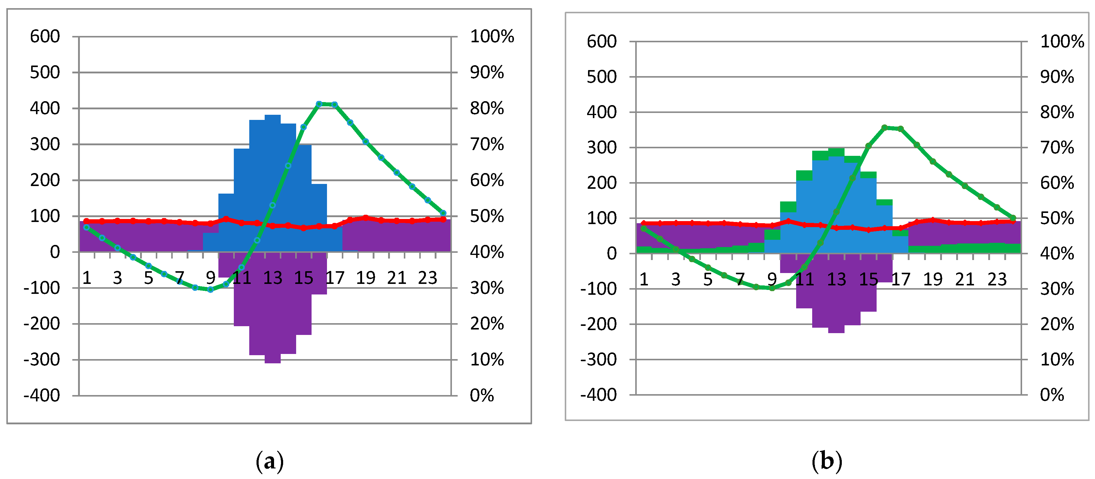
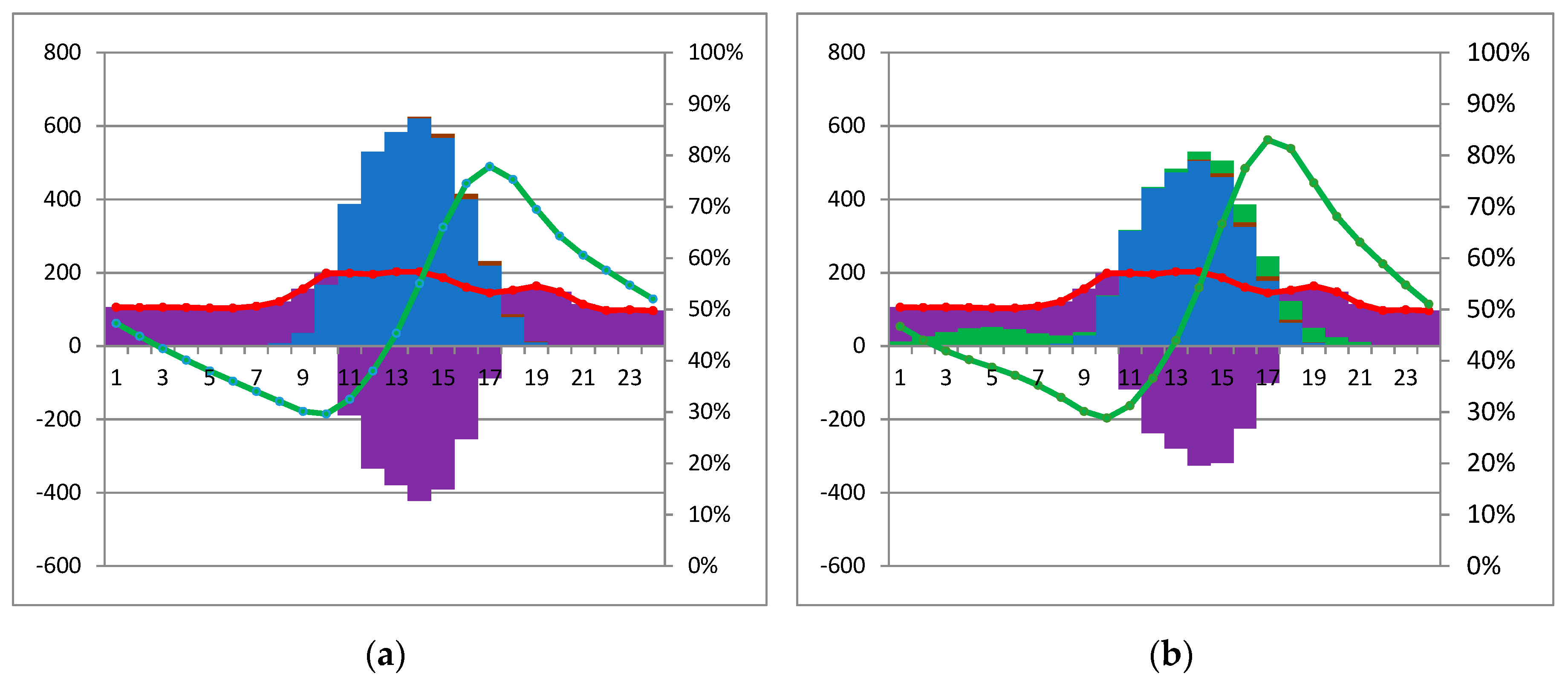
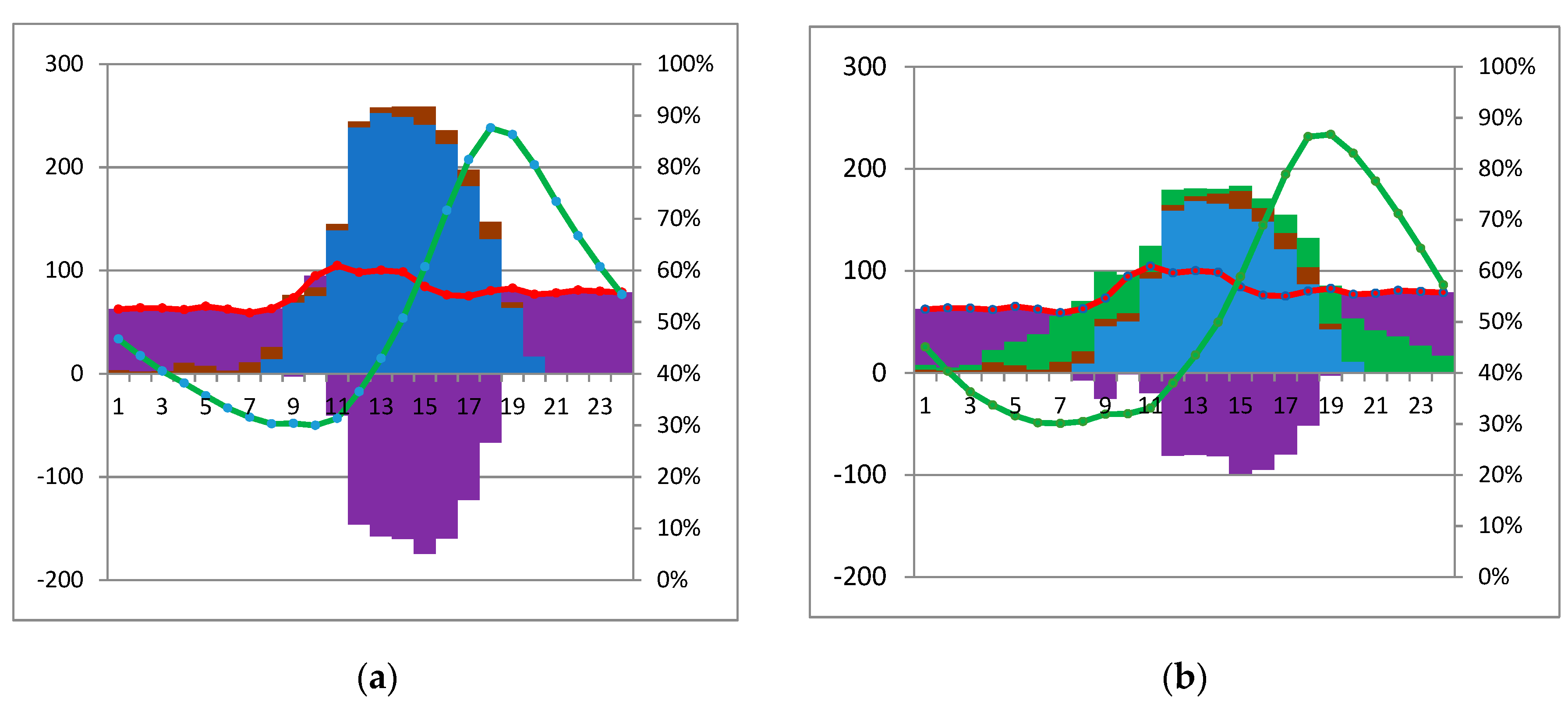
We used the optimum configurations for each load profile, as obtained in the previous section, to calculate the energy mix for each load profile studied, with and without the use of tidal energy (Figure 5, Figure 6, Figure 7, Figure 8, Figure 9 and Figure 10) using the models that are described in Section 3 to further illustrate the effect of the tidal energy on an autonomous RES microgrid with PV and storage.
The red line marks the load curve of the specific day, while the green one marks the SOC, in %, as indicated on the right hand axis. The kW contributed by the PVs, WT, batteries, and TT each hour of the day are shown with respect to the left hand axis, and their respective energy share is color coded: blue for PVs, purple for batteries, maroon for WT, and green for TT. The horizontal axis represents the time of day in hours.
The simulations demonstrate the effect of the tidal energy on the PV and battery sizing and corroborate the results that are shown in Table 3.
The total capital cost is reduced by 5.6%, 15.2%, 4.3%, 12.8%, 6.5%, and 9.5% for Days 1,…, 6, respectively, and the LCE is reduced by 4.5%, 26.9%, 1.2%, 10.9%, 4.3%, and 6.8%, respectively. The most favorable scenario for the use of a tidal generator in a RES microgrid is that of Day#2, which has a high load factor, 0.87, and an average daily demand, 83.09 kW, comparable to the 100 kW nominal power of the tidal generator. Note that, on Day#2, the tidal energy that is generated has the lowest value. The least favorable scenario is that of Day#3, which is also characterized by low tidal energy potential, but also has a low load factor of 0.63 and average daily demand of 216.95 kW, which is double the nominal power of the tidal generator.
7. Conclusions—Future Work
We have demonstrated the effect and role of a periodic power source, such as a tidal turbine, on the performance and sizing of an autonomous hybrid microgrid with photovoltaic panels and storage. The actual data of six different load curves, corresponding to the Euripus campus of the National & Kapodistrian University of Athens in Greece, with the respective meteorological data, have been used to find the optimum combination of RES and storage units for zero load shedding, with and without tidal energy in the mix. The use of tidal energy in a RES microgrid may be used to satisfy the base load requirements, thus reducing the installed capacities of intermittent RES and storage. The impact is more significant for load curves with high load factor. This suggests that the benefits from using tidal energy may be maximized when combined with the demand response mechanisms, even for tidal currents of low velocities.
Future work might involve the use of more detailed models to account for the losses due to inverter performances and battery cycling losses and the implementation of genetic optimization algorithms and multiobjective optimization to investigate the performance of such a microgrid when operating in the grid-connected mode. The proposed microgrid may be a promising solution for regions where low velocity tidal and marine currents exist along with substantial solar and/or wind energy potential, such as the Mediterranean coast line and islands.
Author Contributions
Conceptualization, A.K.; Data curation, A.A. and S.V.; Formal analysis, A.K. and S.V.; Funding acquisition, C.M.; Investigation, A.A.; Methodology, A.K., C.M., S.V.; Resources, C.M.; Software, A.A.; Supervision, A.K.; Validation, A.A. and C.M.; Visualization, C.M.; Writing—original draft, A.A.; Writing—review & editing, A.K. and C.M.
Funding
This research received no external funding.
Acknowledgments
This work was carried out exclusively at the Energy Systems Laboratory in the framework of the MSc in “Intelligent Management of Renewable Energy Systems” which also covered the costs to publish in open access.
Conflicts of Interest
The authors declare no conflict of interest.
References
- Kroposki, B.; Lasseter, R.; Ise, T.; Hatziargyriou, N.D. Making microgrids work. IEEE Power Energy Mag. 2008, 6, 40–53. [Google Scholar] [CrossRef]
- Krishna, K.S.; Kumar, K.S. A review on hybrid renewable energy systems. Renew. Sustain. Energy Rev. 2015, 52, 907–916. [Google Scholar] [CrossRef]
- Sinha, S.; Chandel, S.S. Review of recent trends in optimization techniques for solar photovoltaic–wind based hybrid energy systems. Renew. Sustain. Energy Rev. 2015, 50, 755–769. [Google Scholar] [CrossRef]
- Siddaiah, R.; Saini, R.P. A review on planning, configurations, modeling and optimization techniques of hybrid renewable energy systems for off grid applications. Renew. Sustain. Energy Rev. 2016, 58, 376–396. [Google Scholar] [CrossRef]
- Koutroulis, E.; Kolokotsa, D.; Potirakis, A.; Kalaitzakis, K. Methodology for optimal sizing of stand-alone photovoltaic/wind-generator systems using genetic algorithms. Solar Energy 2006, 80, 1072–1088. [Google Scholar] [CrossRef]
- Diaf, S.; Diaf, D.; Belhamel, M.; Haddadi, M.; Louche, A. A methodology for optimal sizing of autonomous hybrid PV/wind system. Energy Policy 2007, 35, 5708–5718. [Google Scholar] [CrossRef]
- Kaabeche, A.; Belhamel, M.; Ibtiouen, R. Sizing optimization of grid-independent hybrid photovoltaic/wind power generation system. Energy 2011, 36, 1214–1222. [Google Scholar] [CrossRef]
- Li, J.; Wei, W.; Xiang, J. A Simple Sizing Algorithm for Stand-Alone PV/Wind/Battery Hybrid Microgrids. Energies 2012, 5, 5307–5323. [Google Scholar] [CrossRef] [Green Version]
- Yang, H.; Lu, L.; Zhou, W. A novel optimization sizing model for hybrid solar-wind power generation system. Solar Energy 2007, 81, 76–84. [Google Scholar] [CrossRef]
- Ashok, S. Optimized model for community-based hybrid energy system. Renew. Energy 2007, 32, 1155–1164. [Google Scholar]
- Yang, H.; Zhou, W.; Lu, L.; Fang, Z. Optimal sizing method for stand-alone hybrid solar-wind system with LPSP technology by using genetic algorithm. Solar Energy 2008, 82, 354–367. [Google Scholar] [CrossRef]
- Tégani, I.; Aboubou, A.; Ayad, M.Y.; Becherif, M.; Saadi, R.; Kraa, O. Optimal sizing design and energy management of stand-alone photovoltaic/wind generator systems. Energy Procedia 2014, 50, 163–170. [Google Scholar] [CrossRef]
- Fetanat, A.; Ehsan, K. Size optimization for hybrid photovoltaic-wind energy system using ant colony optimization for continuous domains based integer programming. Appl. Soft Comput. 2015, 31, 196–209. [Google Scholar] [CrossRef]
- Maleki, A.; Pourfayaz, F. Optimal sizing of autonomous hybrids photovoltaic/wind/battery power system with LPSP technology by using evolutionary algorithms. Solar Energy 2015, 115, 471–483. [Google Scholar] [CrossRef]
- Seigneurbrieux, J.; Robin, G.; Ahmed, H.B.; Multon, B. Optimization with energy management of PV battery stand-alone systems over the entire life cycle. In Proceedings of the 21st European Photovoltaic Solar Energy Conference and Exhibition, Dresden, Germany, 4–8 September 2006. [Google Scholar]
- Liu, X.; Chen, H.-K.; Huang, B.-Q.; Tao, Y.-B. Optimal Sizing for Wind/PV/Battery System Using Fuzzy c-Means Clustering with Self-Adapted Cluster Number. Int. J. Rotating Mach. 2017, 2017, 9. [Google Scholar] [CrossRef]
- Hakimi, S.M.; Moghaddas-Tafreshi, S.M. Optimal sizing of a stand-alone hybrid power system via particle swarm optimization for Kanauji area in South-East of Iran. Renew. Energy 2009, 34, 1855–1862. [Google Scholar] [CrossRef]
- Hassanzadeh Fard, H.; Bahreyni, S.A.; Dashti, R.; Shayanfar, H.A. Evaluation of Reliability Parameters in Micro-Grid. Iran. J. Electr. Electron. Eng. 2015, 11, 127–136. [Google Scholar]
- Katsigiannis, Y.A.; Georgilakis, P.S. Hybrid Simulated Annealing-Tabu Search Method for Optimal Sizing of Autonomous Power Systems with Renewables. IEEE Trans. Sustain. Energy 2012, 3, 330–338. [Google Scholar] [CrossRef]
- Kanase-Patil, A.B.; Saini, R.P.; Sharma, M.P. Integrated renewable energy systems for off grid rural electrification of remote area. Renew. Energy 2010, 356, 1342–1349. [Google Scholar] [CrossRef]
- Arabali, A.; Ghofrani, M.; Etezadi-Amoli, M.; Fadali, M.S.; Baghzouz, Y. Genetic-algorithm-based optimization approach for energy management. IEEE Trans. Power Delivery 2013, 281, 162–170. [Google Scholar] [CrossRef]
- Shadmand, M.B.; Balog, R.S. Multi-Objective Optimization and Design of Photovoltaic-Wind Hybrid System for Community Smart DC Microgrid. IEEE Trans. Smart Grid 2014, 55, 2635–2643. [Google Scholar] [CrossRef]
- Wang, L.; Singh, C. Multi criteria design of hybrid power generation systems based on a modified particle swarm optimization algorithm. IEEE Trans. Energy Convers. 2009, 241, 163–172. [Google Scholar] [CrossRef]
- Katsigiannis, Y.A.; Georgilakis, P.S.; Karapidakis, E.S. Multi objective genetic algorithm solution to the optimum economic and environmental performance problem of small autonomous hybrid power systems with renewables. Renew. Power Gener. 2010, 4, 404–419. [Google Scholar] [CrossRef]
- Ktena, A.; Manasis, C.; Bargiotas, D.; Katsifas, V.; Soukissian, T.; Kontoyiannis, H. Energy Potential of Euripus’ Gulf Tidal Stream. In Proceedings of the 6th International Conference on Information, Intelligence, Systems and Applications (IISA), Corfu, Greece, 6–8 July 2015; pp. 1–6. [Google Scholar] [CrossRef]
- Ktena, A.; Manasis, C.; Bargiotas, D.; Katsifas, V.; Soukissian, T.; Kontoyiannis, H. Estimation of the Energy Potential of the Euripus’ Gulf Tidal Stream Using Channel Sea-surface Slope. Int. J. Monit. Surveill. Technol. Res. 2015, 3, 23–42. [Google Scholar] [CrossRef]
- Obara, S.; Kawai, M.; Kawae, O.; Morizane, Y. Operational planning of an independent microgrid containing tidal power generators, SOFCs, and photovoltaics. Appl. Energy 2013, 102, 1343–1357. [Google Scholar] [CrossRef]
- Javidsharifi, M.; Niknam, T.; Aghaei, J.; Mokryani, G. Multi-objective short-term scheduling of a renewable-based microgrid in the presence of tidal resources and storage devices. App. Energy 2018, 216, 367–381. [Google Scholar] [CrossRef] [Green Version]
- Kontoyiannis, H.; Panagiotopoulos, M.; Soukissian, T. The Euripus tidal stream at Halkida/Greece: a practical, inexpensive approach in assessing the hydrokinetic renewable energy from field measurements in a tidal channel. J. Ocean Eng. Mar. Energy 2015, 1, 325–335. [Google Scholar] [CrossRef] [Green Version]
- Vika, H.B. Modelling of Photovoltaic Modules with Battery Energy Storage in Simulink/Matlab. Master Thesis, Norwegian University of Science and Technology, Trondheim, Norway, 2014. [Google Scholar]
Figure 1.
The block diagrams of the (a) actual Energy Systems Laboratory microgrid (b) modeled microgrid.
Figure 1.
The block diagrams of the (a) actual Energy Systems Laboratory microgrid (b) modeled microgrid.

Figure 2.
The optimization algorithm of the hybrid autonomous microgrid.

Figure 3.
Measured (solid line) and simulated (dotted line) load curves for six different days of the year.
Figure 3.
Measured (solid line) and simulated (dotted line) load curves for six different days of the year.

Figure 4.
Data used as input to renewable energy systems (RES) models (a) Solar irradiance, in W/m2; (b) Temperature, in °C; (c) Wind velocity, in m/s; and, (d) Tidal current velocity, in m/s.
Figure 4.
Data used as input to renewable energy systems (RES) models (a) Solar irradiance, in W/m2; (b) Temperature, in °C; (c) Wind velocity, in m/s; and, (d) Tidal current velocity, in m/s.

Figure 5.
Day 1, 25/02/2009: Energy balance (a) without and (b) with tidal energy.

Figure 6.
Day 2, 03/01/2009: Energy balance (a) without and (b) with tidal energy.

Figure 7.
Day 3, 01/04/2009: Energy balance (a) without and (b) with tidal energy.

Figure 8.
Day 4, 16/10/2009: Energy balance (a) without and (b) with tidal energy.

Figure 9.
Day 5, 04/06/2009: Energy balance (a) without and (b) with tidal energy.

Figure 10.
Day 6, 10/08/2009: Energy balance (a) without and (b) with tidal energy.


Table 1.
Explanation of symbols used in the flow chart of Figure 2.
Table 1.
Explanation of symbols used in the flow chart of Figure 2.
| Symbol | Explanation | Symbol | Explanation |
|---|---|---|---|
| j = 1,…, 3 | Iteration number | i = 1,…, 24 | Hour of day |
| G | Solar irradiation, in W/m2 | T | Temperature, in °C |
| vw | Wind velocity, in m/sec | PL | Load, in kW |
| Ppv | PV power, in kW | Pwt | WT power, in kW |
| SOC | Battery State Of Charge, in % | Pb | Power from batteries, in kW |
| Pg | Total power generated, in kW | P | Difference between generated power and load demand: P =Pg − PL, in kW |
| Pother | Power from other controllable sources or the grid, in kW | vt(i) | Tidal current velocity, in m/s |
Table 2.
The six load curves studied.
| Day# | dd/mm/yyyy | Season | Season Demand |
|---|---|---|---|
| Day 1 | 25/02/2009 | winter | High |
| Day 2 | 03/01/2009 | winter | Low |
| Day 3 | 01/04/2009 | spring | Typical |
| Day 4 | 16/10/2009 | fall | Typical |
| Day 5 | 04/06/2009 | summer | High |
| Day 6 | 10/08/2009 | summer | Low |
Table 3.
Optimum photovoltaic (PV)-battery combination for the 6 load profiles with and without tidal energy.
Table 3.
Optimum photovoltaic (PV)-battery combination for the 6 load profiles with and without tidal energy.
| Day | Season | Eload (kWh) | Pmax (kW) | Pave (kW) | Load Factor | PV (kW) | PV Capacity Reduction (%) | PV (kWh) | Batteries (kWh) | Battery Capacity Reduction (%) | Tidal (kWh) | Tidal/Load |
|---|---|---|---|---|---|---|---|---|---|---|---|---|
| 2 | Winter | 1994.20 | 95.2 | 83.09 | 0.87 | 637.5 | 28.00 | 2175.97 | 1368 | 19.30 | 0 | 0 |
| 459.0 | 1566.7 | 1104 | 533.85 | 0.27 | ||||||||
| 6 | Summer | 1862.34 | 104.7 | 77.60 | 0.74 | 229.5 | 33.33 | 1894.62 | 888 | 37.84 | 0 | 0 |
| 153.0 | 1263 | 552 | 571.62 | 0.31 | ||||||||
| 4 | Autumn | 3373.23 | 202.9 | 140.55 | 0.69 | 816.0 | 18.75 | 3611.19 | 1968 | 29.27 | 0 | 0 |
| 663.0 | 2934.09 | 1392 | 597.64 | 0.18 | ||||||||
| 1 | Winter | 6295.63 | 383.5 | 262.31 | 0.68 | 1198.5 | 10.64 | 6688.9 | 2688 | 12.50 | 0 | 0 |
| 1071.0 | 5977.31 | 2352 | 634.14 | 0.10 | ||||||||
| 3 | Spring | 5206.87 | 342.2 | 216.95 | 0.63 | 790.5 | 12.90 | 5549.05 | 2232 | 9.68 | 0 | 0 |
| 688.5 | 4833.03 | 2016 | 538.33 | 0.10 | ||||||||
| 5 | Summer | 4595.32 | 314.7 | 191.47 | 0.61 | 535.5 | 14.29 | 4792.04 | 1728 | 26.39 | 0 | 0 |
| 459.0 | 4107.47 | 1272 | 575.79 | 0.13 |
© 2019 by the authors. Licensee MDPI, Basel, Switzerland. This article is an open access article distributed under the terms and conditions of the Creative Commons Attribution (CC BY) license (http://creativecommons.org/licenses/by/4.0/).
Share and Cite
MDPI and ACS Style
Angelopoulos, A.; Ktena, A.; Manasis, C.; Voliotis, S. Impact of a Periodic Power Source on a RES Microgrid. Energies 2019, 12, 1900. https://doi.org/10.3390/en12101900
AMA Style
Angelopoulos A, Ktena A, Manasis C, Voliotis S. Impact of a Periodic Power Source on a RES Microgrid. Energies. 2019; 12(10):1900. https://doi.org/10.3390/en12101900
Chicago/Turabian StyleAngelopoulos, Angelos, Aphrodite Ktena, Christos Manasis, and Stamatis Voliotis. 2019. "Impact of a Periodic Power Source on a RES Microgrid" Energies 12, no. 10: 1900. https://doi.org/10.3390/en12101900
Note that from the first issue of 2016, this journal uses article numbers instead of page numbers. See further details here.