Coupled Motion Characteristics of Offshore Wind Turbines during the Integrated Transportation Process

A State Key Laboratory of Hydraulic Engineering Simulation and Safety, Tianjin University, No. 135 Yaguan Road, Jinnan District, Tianjin 300350, China
*
Author to whom correspondence should be addressed.
Energies 2019, 12(10), 2023; https://doi.org/10.3390/en12102023
Submission received: 4 April 2019
/
Revised: 16 May 2019
/
Accepted: 21 May 2019
/
Published: 27 May 2019
(This article belongs to the Special Issue Recent Advances in Offshore Wind Technology)
Abstract
:The offshore wind turbine (OWT) supported by bucket foundations can be installed in the integrated transportation process by a dedicated vessel. During the integrated transportation process, the wind turbine is considered as a coupling system with the transport ship, which is easily influenced by waves and storms. In view of the motion response and influential factors, the heave and rock stiffness of the entire floating system was proposed, and then the analytical dynamic motion model of the coupling system was established based on the movement mechanism of the traditional floating body in the wave in this paper. Subsequently, the rationality of the proposed motion model was verified based on the field observation data, with the maximum deviation of the motion responses less than 14%. Further, the influence on the heave and pitch motion of the coupling system considering different factors (vessel speed, wave height, wind speed and wave angle) and the factor sensitivity were discussed by the novel analytical model. It is explained that the heave and pitch motion responses rise with the increase of the wave height and wave angle. Simultaneously, the responses decrease as the vessel speed increases considering sailing along the waves. On the contrary, the responses show an obvious increasing trend with the increase of vessel speed in the case of the top wave sailing. In addition, it is also illustrated that the wave height has the greatest influence on the heave and pitch motion responses, followed by the vessel speed. The wave angle has the lowest sensitivity when the heave and pitch motion are far away from its harmonic resonance region.
1. Introduction
Offshore wind energy has become the focus of renewable energy development due to its enormous energy potential, high wind speed, low turbulence and no occupation of cultivated land. In 2018, the global installed capacity of offshore wind power was 4.5 GW, and the cumulative installed capacity has reached 23.1 GW. Simultaneously, the cumulative installed capacity of offshore wind power in China has reached 4.6 GW by the end of 2018 and accounts for 20% of the global offshore wind power market, which shows a good development trend [1].
However, the transportation and installation costs of offshore wind turbines (OWT) are almost up to twice than the cost of onshore wind turbines, which restricts the development of the offshore wind industry. As shown in Figure 1a,b, the offshore wind power installation is mainly divided into the split installation and overall installation [2]. The split installation always needs long construction time offshore and special installation equipment with a higher cost and lower efficiency, which is susceptible to environmental conditions such as wind and waves during the installation. Even a small wag of the conventional crane vessel may lead to an obvious deviation at the nacelle height [3]. At present, the vast majority of overall installation is achieved by a separate installation process including the upper structure (blades, nacelle and tower) and the foundation. Specially, the complex overall installation process is sensitive to weather conditions with a high risk and is not suitable for long-distance transportation. In order to achieve high efficiency and low-cost development of offshore wind power, Lian et al. proposed a novel bucket foundation structure with the advantages of high load capacity [4], self-floating ability [5] and low costs. Additionally, as a good alternative for the conventional transportation and installation of OWTs, one step installation technique of the proposed bucket foundation structure, which includes the onshore prefabrication of foundation, onshore installation and debugging of wind turbine, integrated transportation and installation of the whole wind turbine [6], has been applied in the actual offshore wind farm, as shown in Figure 1c. Although these novel bucket foundations are a rather small proportion of the installed OWTs, it is worth promoting. After this technique is industrialized, the cost will be around 30% lower than that of existing relevant technique, which will make this novel foundation widely applied in OWTs [7]. The purpose of this paper is to investigate the motion behaviors and influential factors of the integrated transportation process, which can provide guidance for further research on the integrated transportation of OWTs supported by these novel bucket foundations.
At present, one of the major challenges of one step installation technology is the integrated transportation of overall OWT on the novel bucket foundation, including the blades, nacelle, tower and foundation. During the transportation process, the coupling system, which combines the wind turbine with the vessel, is susceptible to the external environmental loads because the former structure is considered as an air-floating structure, and the dedicated vessel belongs to the actual floating structure. Considering the wind turbine as a high-rise structure, the dynamic response of the nacelle is often intense which affects the safety and stability of the coupling structural system during the transportation. Therefore, it is of great significance to study the dynamic characteristics of the coupling system of the wind turbine on the novel bucket foundation and the vessel during the integrated transportation process. Moreover, there remains a need to investigate influential factors of safety for the integrated transportation. Since the one step installation method of OWTs was proposed, Zhang and Ding [8] established a numerical model of suction bucket foundation to study the hydrodynamic characteristics of foundations in the towing process. The results show that the subdivision of the bucket can contribute to the stability of foundation. The hydrodynamic responses of the large floater with aircushions depend not only on the wave conditions, but also on the mass of the water column, air cushion height, and air pressure distribution [9]. Subsequently, the numerical model of the whole system was established by the hydrodynamic software MOSES and the influence of the draft and aircushions on the dynamic characteristics of the system was studied. It is concluded that a smaller draft and a greater air cushion in the foundation are beneficial to a safe transportation process [10]. Afterwards, Zhang et al. also conducted a series of field experiments to study the effects of air pressure inside the bucket foundation and ballasts in the vessel on the stability of transportation [3]. The results show that the vessel is quite stable during wet tows. However, a larger draft and smaller air pressure makes the vessel less stable. In addition, the ballast in the vessel may have little effect on the stability. Huang also used the software MOSES to simulate the transport vessel carrying two novel bucket foundations together with the upper offshore wind turbines and analyzed the influence factors of motion response [11]. The results of simulations show that wave height has a great impact on the integrated transportation.
Generally speaking, most of the previous studies were completed based on numerical simulations and were lack of theoretical analyses and field measurement data obtained from the transportation process. In this paper, an analytical motion model of the coupling system, which combined the overall OWT on the novel bucket foundation with vessel during the transportation process, was established by both the theoretical derivation method and field measurement data analysis. Then, the effect and the sensitivity of various factors (vessel speed, wave height, wind speed and wave angle) on heave and pitch motion of the system were further studied based on the proposed model. Firstly, the field measurement of integrated transportation process is introduced in Section 2. Secondly, the heave and rock stiffness of the coupling system are theoretically derived, and the additional water correction coefficient of heave and rock is solved according to the field observation data in Section 3. Then, the rationality of the established motion equation of the system is verified based on the observation data. Thirdly, the influences of factors on the motion of the whole system are analyzed by the established analytical motion model in Section 4. Finally, the sensitivity of each factor (vessel speed, wave height, and wave angle) on the heave and pitch motion of the entire system is studied in Section 5.
2. Prototype Observation of the Integrated Transportation
2.1. The Dedicated Transportation Vessel
The dedicated transportation vessel for the suction bucket foundation is a special supporting ship in one step transportation of the OWT, which is mainly used for the integrated transportation of nacelle, blades, tower and foundation based on the structural self-floating ability, as shown in Figure 1c. The vessel is a box-shaped structure, and the bow and the stern are provided with a semi-circular recess for accommodating the bucket foundation of the wind turbine. The novel bucket foundation consists of a steel bucket with 30.0 m diameter and 12 m height, pre-stressed concrete transition part with 20 m height, which is about 2700 t in the total weight. During this measured transportation, only one OWT supported by suction bucket foundation was carried. The main design parameters of the vessel and wind turbine are shown in Table 1.
2.2. Arrangement of the Field Measurement
The destination of this measured transportation process is one offshore wind farm which is 10 km off the coast of the Yellow Sea in China, with the water depth of 8–12m. The transport route and the installation location are shown in Figure 2. In order to monitor the motion of the vessel and the wind turbine during the transportation, six three-directional displacement sensors with the lowest frequency of 0.1 Hz in each measured station were used to acquire the low-frequency and multi-directional dynamic signals of the coupling structural system at the sampling frequency of 300 Hz. The observation points and sensors are illustrated in Figure 3.
Specially, the measured point D6 was arranged on the vessel compared with the others D1–D5 located on the OWT. Additionally, the X (left and right chord direction of the vessel) and Z (the longitudinal chord direction of the vessel) directions are horizontal and Y (vertical ground direction) direction is vertical. The Y-direction motion displacement represents the heave displacement of the system. X-direction and Z-direction motion displacement can be approximated to indicate the change in the roll angle and pitch angle of the entire system, respectively. From 8th June to 10th June in 2017, the variables such as vessel speed, wave height, and wind speed were recorded every half hour. In Figure 4, data of vessel speed, wave height, and wind speed for nearly 30 hours during the transportation is given. The vessel speed varied between 0 and 6 knots. At the same time, the wave height varied between 0.1 m and 0.6 m, while the wind speed ranged from 0 to 11 m/s.
3. Motion Model of the Coupling System Considering Regular Wave Effect
3.1. Elastic Stiffness of the Coupling System
3.1.1. Heave Elastic Stiffness
The displacement of the entire system in six degrees of freedom (surge, sway, heave, roll, pitch and yaw) can be expressed as , respectively. Due to the absence of external constraints, only the heave, roll and pitch may lead to the volume change of the air cushion inside the suction bucket foundation among the motion of six degrees of freedom in the whole floating structure system. Therefore, the coupling system can generate resistance in these three degrees of freedom, and the stiffness matrix can be obtained as:
where, is the stiffness coefficient of restoring force.
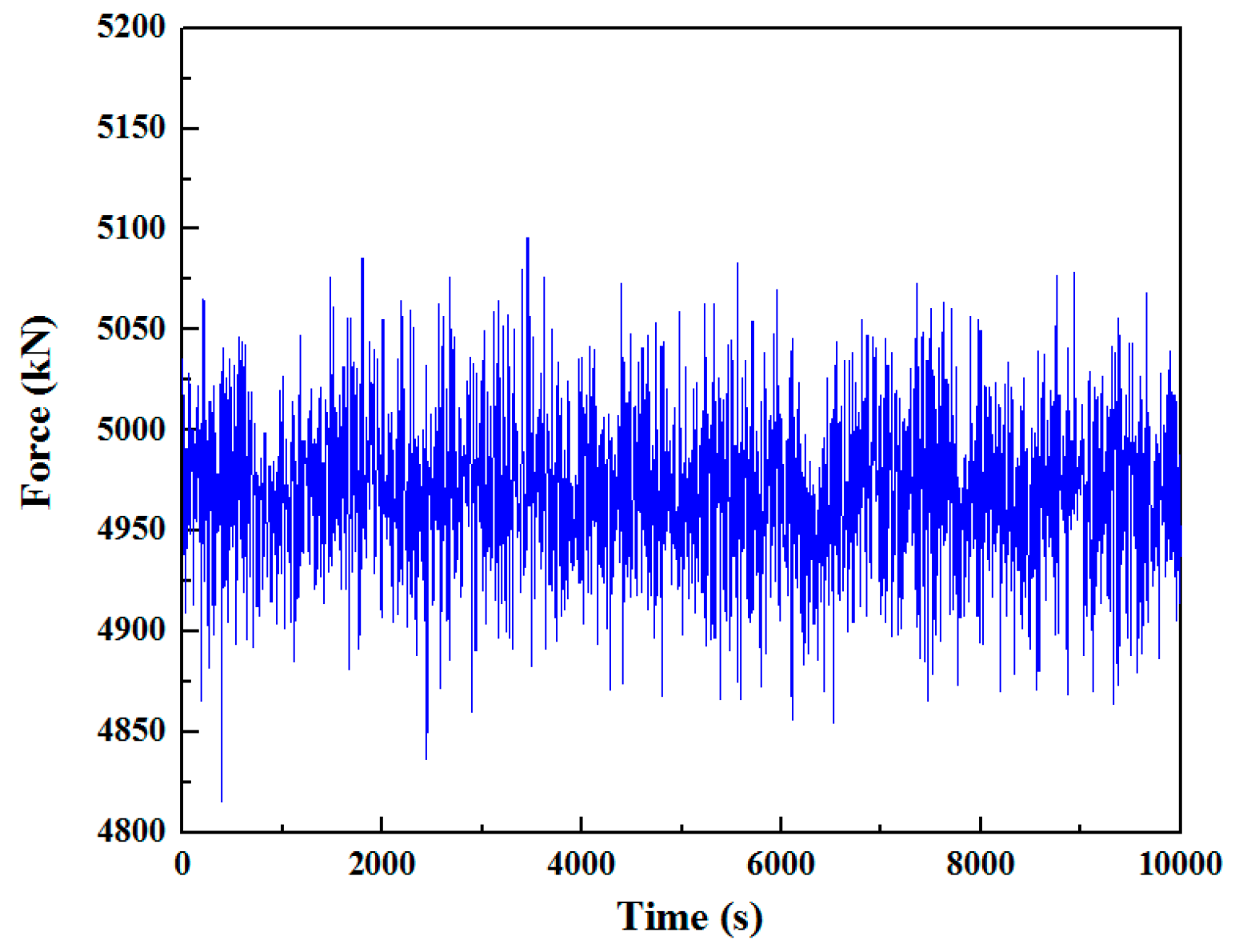
During the transportation process, the pre-installed pressure sensor was used to monitor the force between the vessel and foundation, and the measured results are shown in Figure 5.
As described in Figure 5, the bonding force between the vessel and foundation always keeps at least 4800 kN with the fluctuation of force less than 300 kN to ensure the tight coupling between the vessel and foundation during the whole transportation process. Thus, the heave elastic stiffness of the coupling floating system can be considered as a whole, as shown in Figure 6. It can also be explained that the spring stiffness of air cushion inside the bucket foundation is the series coupling of the water spring and the air spring, and the heave elastic stiffness of the whole system is equivalent to the parallel coupling of heave stiffness of both the whole wind turbine and the vessel. The stiffness of water spring in bucket foundation can be calculated by the product of the water gravity and the area of waterline surface. The air spring stiffness of the air cushion can be expressed as the following [12]:
where, is the area of air cushion, is the air pressure inside foundation, and is the air column height inside foundation.
Hence, the heave elastic stiffness of the coupling system can be expressed as:
where, is heave elastic stiffness of the vessel, is the water spring stiffness of foundation,, is the unit weight of sea water, is the water spring stiffness of air cushion, , is the stiffness coefficient in heave.
Compared with the whole coupling system, the skirt thickness of the bucket foundation is so small that the water spring stiffness of the foundation can be negligible. Equation (3) may be simplified as:
During the transportation process, only the air spring stiffness will change as the air pressure inside the bucket foundation changes. When the stiffness of the air spring increases, the heave elastic stiffness of the system increases based on Equation (4).
Further, the seal height of the seven rooms inside the bucket foundation during one transportation period is analyzed and described in Figure 7. The seal height can keep steady for the whole duration of the transport by adjusting the air pressure of each subdivision of foundation.
As shown in Figure 7, it can be considered that the air pressure inside the bucket foundation stays constant because the internal liquid seal height always retains more than 2.6 m with the liquid level fluctuation of each room inside the foundation retaining less than 20 cm during the transportation process. Consequently, if the air pressure inside the foundation and the air column height inside the foundation do not change, the corresponding air spring stiffness of the air cushion and the heave elastic stiffness of the system will both remain stable according to Equation (4).
3.1.2. Rock Elastic Stiffness
When the seal height of the rooms inside the bucket foundation remains constant, it can also be considered that the rocking stiffness of the coupling system will not obviously change during the transportation process. When the coupling system is tilted θ around the Y axis, its rocking schematic is shown in Figure 8.
Rolling inertia moment of the suction bucket foundation is expressed as [12]:
Similarly, the pitching moment of inertia is expressed as:
where, is the air-floating reduction factor, is the mass quality of bucket foundation with the upper wind turbine, and , are the gravity center coordinate of the wind turbine with bucket foundation in the entire motion coordinate system.
Since the skirt thickness of the bucket foundation can be negligible, Equations (5) and (6) can be rewritten as:
Consequently, the transverse stability arm and longitudinal stability arm of the entire system can be given as:
where, is the rolling inertia moment of the bucket foundation, is the rolling inertia moment of the vessel, is the pitching inertia moment of the bucket foundation, is the pitching inertia moment of the vessel, and is the volume.
The transverse metacentric height and longitudinal metacentric height can be obtained as:
where, are the Z-direction coordinates of the gravity center and the floating center of the system, respectively.
Consequently, the stiffness associated with the rocking motion of the coupling system can be obtained as:
where, is the density of sea water, are the center coordinates of the waterline surface of the vessel, are the center coordinates of the waterline surface of the foundation, and are the center coordinates of the waterline surface of the air cushion inside the bucket foundation, are the stiffness coefficient.
3.2. Additional Water Correction Coefficient of the Coupling Floating System
The additional water correction coefficient is essential to theoretically derive the motion equation of the floating system. It can be defined as the ratio of the total mass (including the mass of the water driven by the floating body) to the mass of the floating body during the movement of the system. Additionally, the additional water correction coefficient is influenced by the shape of the floating structure, air pressure inside the bucket foundation, and the draft. In view of the fact that the entire floating system can be regarded as a coupling system composed of an air-floating structure and a real floating body structure, the theoretical analysis and derivation on the additional water correction coefficient of the entire structure are complicated and difficult. Therefore, the additional water correction coefficient of the entire system can be derived from the frequency domain analysis of the field observation data in combination with the empirical formula.
3.2.1. Additional Water Correction Coefficient for Heaving
Taking the measured point D6 on the vessel as an example, the typical measured heave displacement and its power spectral density of the coupling system during the transportation are respectively described in Figure 9 and Figure 10. According to wave frequency encountered in the offshore wind farm and engineering empirical formula for heave natural period of vessel [13], it can be concluded from Figure 9 and Figure 10 that the natural frequency of the heave motion in the entire system during this period is about 0.16 Hz, and the encounter frequency of wave is likely to be 0.09 Hz.
The total mass of the heave motion in the entire system includes the mass of the system and the mass of the water driven by the system . It can be defined as:
where, is the additional water correction coefficient for heave motion.
According to the kinetic principle, the period of the heave motion of the entire system can be expressed as:
where, is the natural period of heave motion, which can be obtained from field measured data, and is the heave elastic stiffness of the entire system.
Hence, the additional water correction coefficient for heave motion can be obtained by combining Equations (18) and (19):
The additional water correction coefficient of heave motion in the entire system is calculated to be 1.41 based on Equation (20). If the water mass enclosed by the bottom of the bucket foundation is included, the additional water correction coefficient of the heave motion will be 1.29.
3.2.2. Additional Water Correction Coefficient for Rocking
Although the angular change of the system was not measured, the left and right chord (X-direction) motion displacement of the vessel (measured point D6) can be approximated to indicate the change in the roll angle of the entire system. A typical time history and spectrum diagram of the X-direction motion displacement at the measured point D6 are shown in Figure 11 and Figure 12.
Empirical formula for estimating the natural period of roll in engineering can be written as [13]:
where, is the rolling natural period, is the hull width, and is the hull height.
Based on Equation (21), the roll period can be calculated as 5.656 s and the corresponding frequency is 0.177 Hz. Thus, it can be concluded from Figure 12 that the rolling natural frequency of the entire system is 0.17 Hz, and the encounter frequency of wave may be 0.11 Hz.
The total mass inertia moment of the rolling motion of the entire system includes the mass inertia moment of the system and the mass inertia moment of the water driven by the system . It can be defined as:
where, is the additional water correction coefficient of rolling motion.
If the influence of water damping on the roll of the entire system is neglected, the natural period of the rolling motion can be obtained as:
where, is the natural period of roll, which can be obtained from field measured data, and is the roll elastic stiffness of the entire system.
The additional water correction coefficient for rolling motion can be obtained by combining Equations (22) and (23):
The additional water correction coefficient of rolling motion in the entire system is calculated by Equation (24) to be 1.30. If the water mass enclosed by the bottom of the bucket foundation is included, the additional water correction coefficient of the rolling motion will be 1.27. In the same way, this method can also be used to obtain the additional water correction coefficient of pitching motion in the entire system.
3.3. The Motion Equation of the Coupling System during the Integrated Transportation Process
The displacement of the entire system in six degrees of freedom is expressed as . The forces considered in the analysis include the following:
- Inertia force. Considering the influence of the additional water correction coefficient of the system, the inertial force at the i-th degree of freedom can be expressed as:where, is the additional water correction coefficient, and is the mass inertial force coefficient of the system.
- Damping force. It is generally considered to be proportional to the speed and can be expressed as:where, is generalized damping coefficient.
- Resilience. Considering the influence of air cushion inside the bucket foundation, its restoring force can be written as:where, is the stiffness coefficient of restoring force.
- Wave disturbance force. The wave disturbance force during the transportation process is related to the amplitude of the incident wave . The whole system can be simplified into a box-shaped floating body with a rectangular cross-section to calculate the wave force and moment. Thus, the wave force of the entire system can be obtained as:where, is the disturbance force generated by the unit incident wave, which is influenced by wavelength, wave direction, vessel shape and speed, and can be calculated by the slice method, and is the wave encounter frequency.
- Wind load. Due to the high height of the structure, the wind effect on the entire system should be considered during the transportation process. The wind load and wind moments of the coupling system are:where, is the air density, is the surface area of wind load, is the instantaneous wind speed, which can be simulated by the Davenport spectral model, is the wind pressure coefficient, is the wind chord angle, and is the arm of wind moments.
By establishing the equilibrium equation between the above forces, the motion equation of the entire system at the i-th degree of freedom is:
Then, Equation (31) can also be rewritten in matrix form as:
In this paper, the heave and pitch motion of the whole system will mainly be analyzed with the assumption that only the wave damping of the heave motion is considered. Hence, the wave damping coefficient and the wave force (moment) can be expressed as [14]:
where,
where, is the wave amplitude ratio, is the wave frequency, is the wave number, is the damping coefficient, is the vessel speed, is the amplitude, is the half width of water line, and is the average draft of the profile.
From the previous analysis, it can be seen that the correction factors of the coupling system depend on the sea state and type of the vessel. The analytical motion model was derived based on regular waves and was suitable for shallow water area with small wave height.
3.4. Verification of Analytical Motion Model Considering Regular Wave Effect
In order to verify the rationality and applicability on the theoretical analysis of the motion in the coupling floating system, the heave and pitch motion response of the system under six conditions (listed in Table 2) were calculated and solved in the time domain using the Newmark method based on Equation (31). Further, the comparisons between the theoretical responses and the measured data obtained from the transportation period were also completed and discussed in Figure 13, Table 3 and Table 4 in time and frequency domains, respectively.
As shown in Figure 13, the responses obtained by the two methods are similar in both time and frequency domains. It can be found that the maximum deviation of the response amplitude was about 13.03%, while the frequency deviation is controlled at 16.38%, as listed in Table 3 and Table 4. Moreover, it can be found in Table 3 that the minimum deviation of the response amplitude and the root mean square (RMS) can reach 0.29%, 0.47%, respectively. It can be observed in Table 4 that the minimum frequency deviation under the six conditions is 3.67%. The deviation varies greatly under different conditions. The average deviation of response amplitude and RMS is 5.21%, 6.08%, respectively, while the average deviation in the frequency domain is 10.05%. Therefore, it was verified that the established analytical model has good rationality based on these results. However, there are still some deviations between the analytical results and the measured data due to the irregularity of the wave, the deviation of the wave angle and the nonlinearity of the air cushion inside the foundation. It is worth noting that the average deviation in the frequency domain is larger than that in the time domain. The possible reason for this difference is attributed to the irregularity of the wave. To be specific, the analytical motion model was derived based on regular waves, while the waves encountered during the integrated transportation are usually irregular.
4. Factor Influence on the Motion of the Whole Transport System
The floating analysis during the integrated transportation process is a complex research on the coupling motion combined the vessel with the wind turbine including blades, tower and foundation. Since the entire system is susceptible to wind and wave loads due to the complicated external conditions, it is necessary to analyze the influence of the main factors (including vessel speed, wave height, wind speed, wave angle, etc.) on the motion responses of the entire system during the transportation process. Hence, the established analytical motion model in Section 3 can be used to analyze the influence of various factors on the heave and pitch motion in the entire floating system.
4.1. Vessel Speed Influence
The frequency of the wave disturbing the vessel is always defined as the encounter frequency. When the vessel is sailing at speed under the regular wave at a wave angle of , the encounter frequency is:
where, is the wave frequency, and is the wave number.
Based on Equation (40), it can be obtained that the vessel speed affects the motion response by the wave encounter frequency.
Afterwards, the heave and pitch motion responses of the system at different vessel speeds, along with the other factors shown in Table 5, are analyzed. Figure 14 shows the time histories and the main period values of heave and pitch motion in the entire system at different vessel speeds, respectively. In addition, the amplitudes of the heave and pitch motion responses change as functions of vessel speed, as shown in Figure 15.
It is worth mentioning that the dedicated vessel speed in the transportation process varies from a low speed range from 0–6 knots. In the case of sailing along the waves, it can be seen that the response period rises with the increase of the vessel speed, as described in Figure 14. It is because that the encounter frequency of wave will change as the vessel speed increases. Additionally, the amplitudes of the heave and pitch response in the entire system decrease with the increase of the vessel speed. The displacement responses at low speed are larger than those at high speed, as shown in Figure 15. Quantitatively, in Figure 15, the displacement response amplitudes of the heave and the pitch reach the maximum values of 10.7 mm and 7.3 rad, respectively, when the vessel speed is zero. When the vessel speed is 6 knots, the amplitudes of the heave and pitch response are 5.6 mm and 4.6 rad, respectively.
The heave and pitch motion responses of the system at different vessel speeds need to be reanalyzed, when the wave angle is 180° (top wave sailing). The time histories of heave and pitch motion in the entire system at different vessel speeds, and the main period values at different speeds are shown in Figure 16. In addition, Figure 17 shows the amplitudes of the heave and pitch motion responses as functions of vessel speed.
In the case of the top wave sailing, the response period decreases with the increase of the vessel speed, as shown in Figure 16, because the encounter frequency of wave changes as mentioned above. As described in Figure 17, within the range of the vessel speed, the amplitudes of the heave and pitch motion responses in the entire system rise with the increase of the vessel speed, and the displacement responses at high speeds are larger than those at low speeds. Since the wave encounter period at high speed is close to the heave and pitch natural period of the whole system, the response amplitudes of the heave and pitch increase rapidly when the vessel speed is approaching 5 knots and 6 knots, respectively, due to the harmonic resonance motion. The maximum amplitude of the heave is 129.8 mm, while that of the pitch is 0.011 rad, as shown in Figure 17. Thus, the vessel speed and the wave angle should be adjusted reasonably according to the wave parameters in order to avoid the occurrence of resonance phenomenon during the transportation process.
4.2. Wave Height Influence
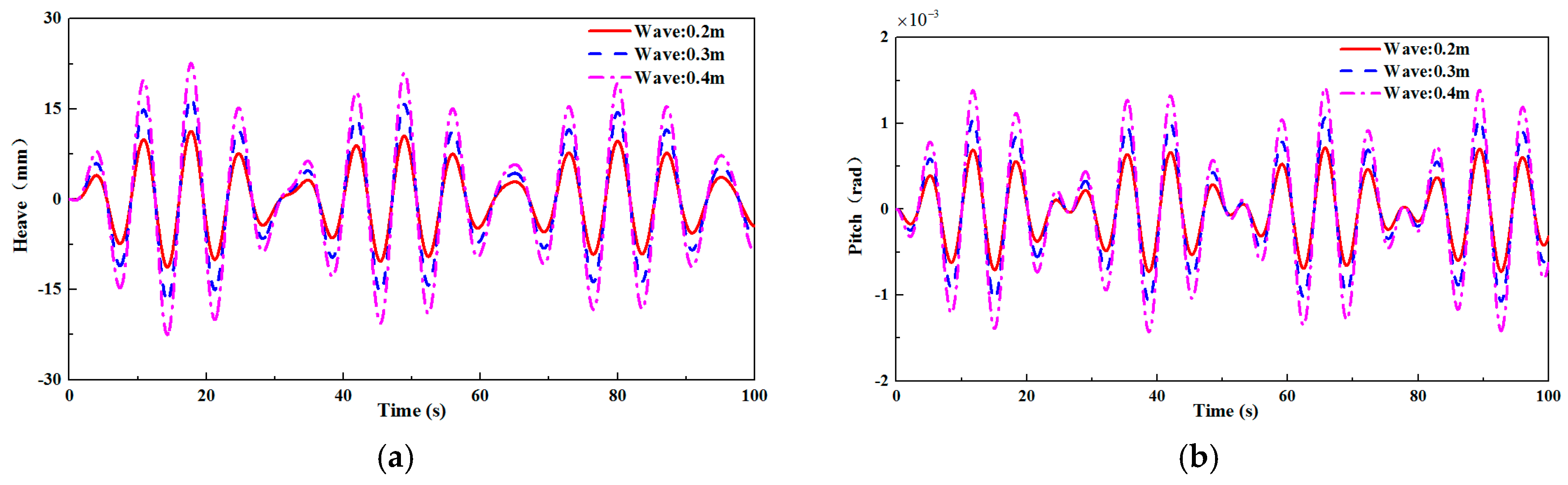
Generally speaking, the entire floating system always receives energy from the waves constantly and results in the heave and pitch motion. Then, the heave and pitch motion response of the system at different wave heights (refer to the wave height in Section 2.2) are analyzed and the corresponding time histories are also described in Figure 18 with the values of other factors listed in Table 6.
It can be seen in Figure 18 that the heave and pitch motion responses increase as the wave height increases, and the response period is not affected by wave height. In addition, the change of the wave angle does not have a significant influence on the conclusions obtained above, which is different from the vessel speed. Therefore, the integrated transportation should be carried in a good sea condition with a small wave height.
4.3. Wind Speed Influence
The heave and pitch motion response of the entire system at different wind speeds are studied and the amplitudes of the heave and pitch motion responses as functions of wind speed are shown in Figure 19, with the other factors listed in Table 7. It is shown that the heave and pitch motion responses have an obvious increasing trend as the wind speed rises. However, the wind speed has less influence on the response of the entire system compared with the vessel speed and wave height. Quantitatively, when the wind speed increases from 1 m/s to 12 m/s, the response amplitude of the heave is only increased by 0.12%, while the amplitude of the pitch is 5.14%. Furthermore, one can conclude that the pitch motion is more sensitive to the wind speed than the heave motion. Actually, there is a correlation between wind speed and wave height that when the wind speed is high, the wave height is usually large. Thus, the high wind speed conditions are often not suitable for the integrated transportation.
4.4. Wave Angle Influence
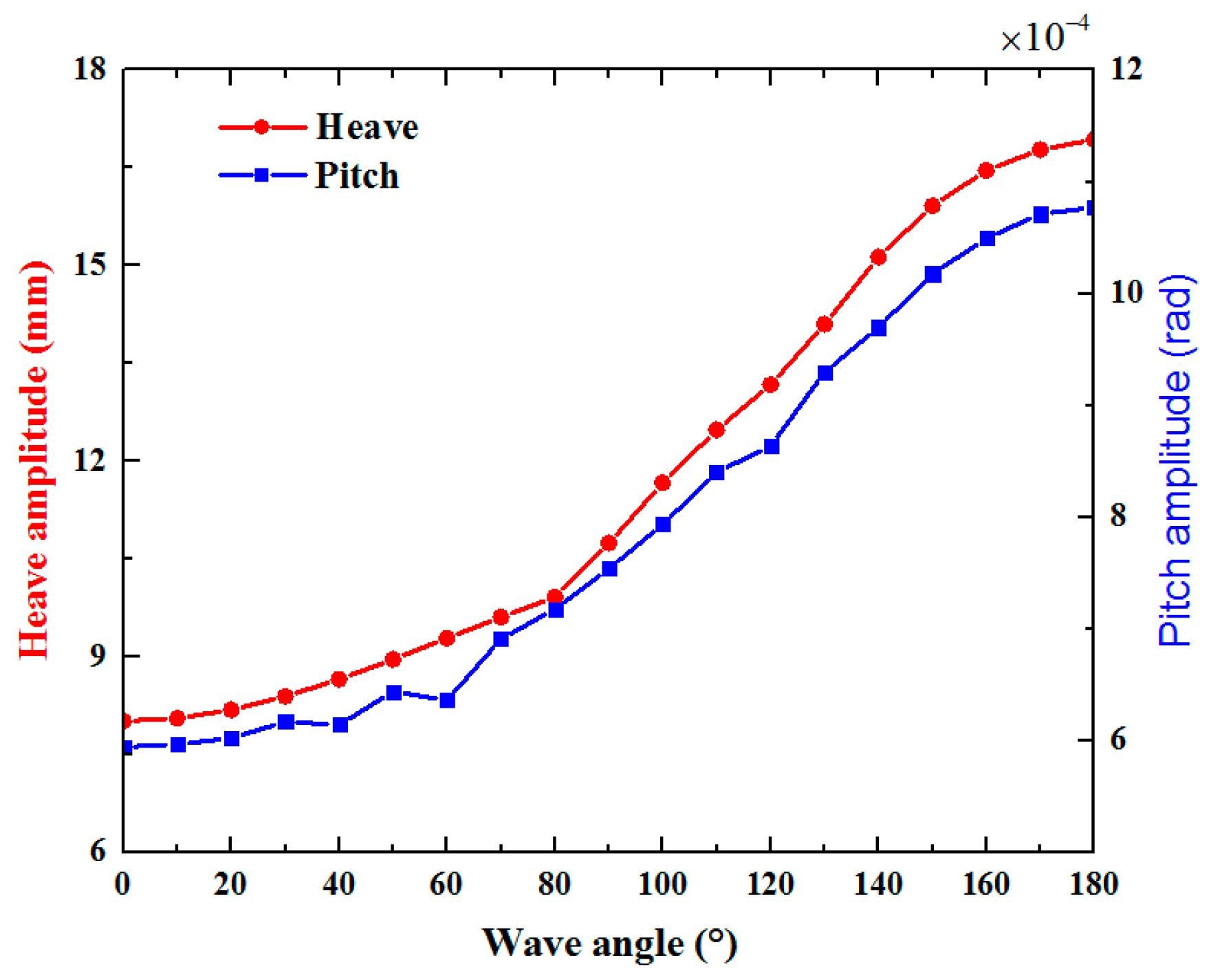
The heave and pitch motion response of the entire system at different wave angle are also analyzed and the other factors are listed in Table 8. Figure 20 shows the time history of heave and pitch motion in the entire system at different wave angles, respectively, and the main period values at different wave angles are also provided. Additionally, the amplitude of the heave and pitch motion response are shown as functions of wave angle in Figure 21.
Figure 20 also shows that the response period decreases with the increase of the wave angle due to the change of wave encounter frequency. Additionally, it is also found in Figure 21 that the amplitude of the heave and pitch motion responses in the entire system will rise with the increase of the wave angle. When the wave angle increases from 0° to 180°, the amplitude of the heave displacement increases from 8.02 mm to 16.94 mm, while the amplitude of the pitch increases from 5.94 rad to 10.77 rad.
5. Factor Sensitivity Analysis
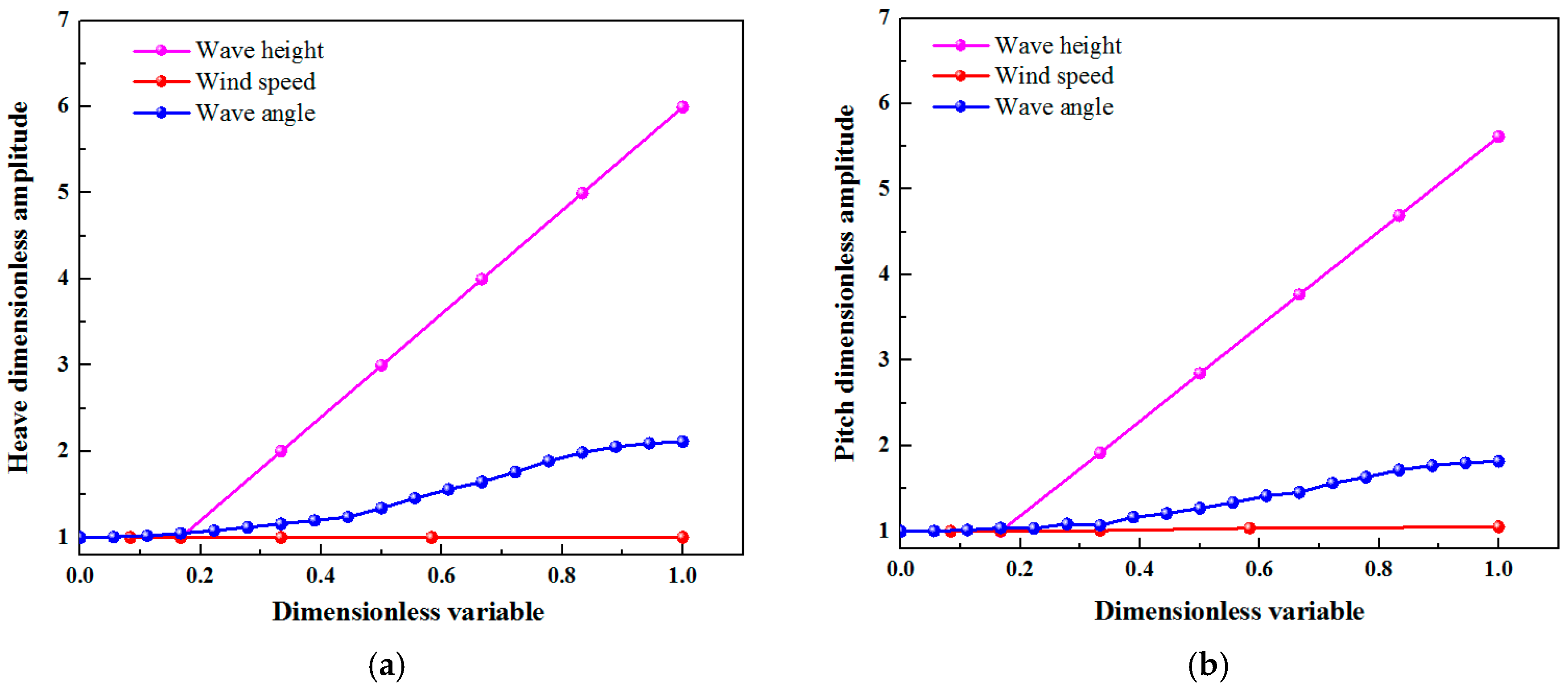
Based on the previous analysis in Section 4, since different factors have different effects on the heave and pitch motion response, it is necessary to normalize the influencing factors to study the sensitivity of the factors. The abscissa of the influencing factor (wave height, wind speed and wave angle) graphs is divided by its maximum value and the ordinate is divided by the minimum value for normalization, as shown in Figure 22. It can be seen in Figure 22 that the influence of the factors on the pitch motion response is consistent with the influence on the heave motion response, and it is easy to find that the motion response is least sensitive to wind speed. The wave height has the greatest influence on the heave and pitch motion responses.
In this section, the gray relational analysis (GRA) method [15] can be used to analyze the sensitivity of the heave response to other factors, including vessel speed , wave height , and wave angle , to find out the important factors affecting the motion response.
5.1. Grey Relational Analysis (GRA)
GRA is part of grey system theory, which is suitable for solving problems with complicated interrelationships between multiple factors and variables [16]. The main procedure of the proposed GRA is presented below [17]:
- Reference sequence definition
The influence factors of the heave response are defined as the subsequence :
Then, it defines the RMS of the heave displacement response under the conditions of subsequence factors as the parent sequence :
- 2.
- Range change of sequence
Since the units vary for different factors, it is necessary to process each factor data to eliminate the influence of the units of each factor on the parent sequence and the subsequence. The method of range change will be used to process by the following equations in this paper:
If the subsequence and the parent sequence are negatively correlated, Equation (44) should be rewritten as:
Subsequently, the following changes are made in the processed sequences to obtain a new difference sequence matrix :
Then take the maximum and minimum values of the new difference sequence for analysis.
- 3.
- Grey relational coefficient and grade calculation
The grey relational coefficient can be calculated by Equation (47):
where, is the distinguishing coefficient, . In this paper, the distinguishing coefficient is set as 0.5, according to the principle of minimum information.
The grey relational grade represents the level of correlation between the reference sequence and the comparability sequence. It varies within the interval [0,1], and the closer the grade is to unity, the more sensitive the parent sequence is to the subsequence; on the contrary, the closer the grade is to zero, the less sensitive it is. The grey relational grade can be obtained by Equation (48):
5.2. Results of Sensitivity Analysis
It is assumed that the heave and pitch motion in the entire system are far away from their harmonic resonance regions, and the wave period remains constant at 9.05 s. Since it is quite different in the case of the top wave sailing and sailing along the waves, the sensitivity analysis using the established analytical model can be divided into two cases. The sensitivity analysis on the case of sailing along the waves will be firstly discussed based on the definition that the change of factors (vessel speed , wave height , wave angle ) is selected as the reference matrix , while the RMS of heave displacement is selected as the comparability matrix .
The two matrices above are subjected to dimensionless processing by Equations (43)–(45), and the relational coefficient matrix L can be obtained by Equation (47):
Then, the grey relational grade can be calculated using Equation (48):
Therefore, it can be concluded that in the case of sailing along the waves, the sensitivity of the influencing factors is ranked as: .
In the case of the top wave sailing, the reference matrix and the comparability matrix can be given as:
The relational coefficient matrix L is then obtained as:
The grey relational grade can be obtained by Equation (48) as:
Therefore, it can be concluded that in the case of the top wave sailing, the sensitivity of the influencing factors is still ranked as: .
Subsequently, the sensitivity of the vessel speed and wave height will be discussed based on the field observation data. It can be approximated as the wave angle and the wave frequency remaining unchanged in the analysis. The reference matrix and the comparability matrix are written as:
Then, the relational coefficient matrix and the grey relational grade are obtained as:
Thus, the sensitivity of these two influencing factors is ranked as: for the RMS of the heave displacement, which is consistent with the results of the sensitivity analysis of the established analytical motion model.
As a summary, when the heave and pitch motion of the entire system are far away from their harmonic resonance regions, the wave height has the greatest influence on the heave and pitch motion response of the floating system, followed by the vessel speed, and the wave angle is the lowest sensitivity in addition to wind speed. Therefore, the sea conditions with small wave heights should be selected for the integrated transportation process (one step transportation) of OWTs supported by bucket foundations.
6. Conclusions
In this paper, the heave and rocking stiffness of the floating system were derived considering the influence of the air cushion inside the bucket foundation of OWTs based on the movement mechanism of the traditional floating body in the wave in order to study the motion responses of the entire coupling system during the integrated transportation process. Subsequently, the influence of various factors including the vessel speed, wave height, wind speed, wave angle on the heave and pitch motion responses of the entire system were also analyzed by the established analytical model. The analytical motion model was derived based on regular waves and was suitable for shallow water area with small wave height. Based on the results and discussions presented, the key conclusions can be obtained as the following:
- (1)
- The proposed analytical model and motion equations were verified to have a good rationality compared with the measured data obtained from one field measurement on the integrated transportation process of the entire OWT structure. The average deviation of the response amplitude and RMS between measurements and analysis results are 5.21% and 6.08%.
- (2)
- In the case of sailing along the waves, the amplitudes of the heave and pitch motion responses of the entire system decrease as the vessel speed increases, while the response period increases. On the contrary, in the case of the top wave sailing, the amplitudes of the heave and pitch responses have obvious increasing tends with the increase of the vessel speed, while the response period decreases. In addition, there is a risk of harmonic resonance motion in the entire system at high vessel speeds. Therefore, the vessel speed should be reasonably controlled, and the vessel should consider sailing along the waves, to avoid the occurrence of the harmonic resonance phenomenon.
- (3)
- The analytical motion model was derived based on regular waves and was suitable for shallow water area with small wave height. As the wave height increases, the amplitudes of the pitch and heave response of the entire system also increase. Although the heave and pitch motion responses increase with the increase of wind speed, the wind speed has less influence on the response of the entire system than other factors such as vessel speed and wave height. Moreover, with the increase of the wave angle, the heave and pitch motion response also shows an increasing trend, while the response period decreases. Therefore, the sea condition with smaller wave height is suitable for the integrated transportation.
- (4)
- The sensitivity of the main factors (vessel speed , wave height , and wave angle ) affecting the heave and pitch motion responses was discussed by gray relational analysis method. The results show that the wave height has the greatest influence on the motion, and the sensitivity of each factor is ranked as: wave height > vessel speed > wave angle.
Author Contributions
Conceptualization, J.L.; formal analysis, J.J. and P.W.; funding acquisition, J.L. and X.D.; methodology, J.J. and X.D.; resources, J.J. and H.Z.; software, J.J.; supervision, J.L., X.D. and H.W.; validation, X.D. and H.W.; writing—original draft, J.J.; writing—review and editing, X.D.
Funding
This research was funded by the National Natural Science Foundation of China (Grant No. 51709202), Innovation Method Fund of China (Grant No. 2016IM030100) and Tianjin Science and Technology Program (Grant No. 16PTGCCX00160).
Acknowledgments
All workers from the State Key Laboratory of Hydraulic Engineering Simulation and Safety of Tianjin University are acknowledged. The writers also acknowledge the assistances of anonymous reviewers.
Conflicts of Interest
The authors declare no conflict of interest.
Abbreviations
| OWT | offshore wind turbine |
| MSL | mean sea level |
| RMS | root mean square |
References
- Global Wind Energy Council (GWEC). Global Wind Report; GWEC: Brussels, Belgium, 2018. [Google Scholar]
- Wang, Y.; Bai, Y. Investigation on installation of offshore wind turbines. J. Mar. Sci. Appl. 2010, 9, 175–180. [Google Scholar] [CrossRef]
- Zhang, P.Y.; Han, Y.; Ding, H.; Zhang, S. Field experiments on wet tows of an integrated transportation and installation vessel with two bucket foundations for offshore wind turbines. Ocean Eng. 2015, 108, 769–777. [Google Scholar] [CrossRef]
- Lian, J.J.; Chen, F.; Wang, H.J. Laboratory tests on soil–skirt interaction and penetration resistance of suction caissons during installation in sand. Ocean Eng. 2014, 84, 1–13. [Google Scholar] [CrossRef]
- Le, C.H.; Ding, H.Y.; Zhang, P.Y. Air-floating towing behaviors of multi-bucket foundation platform. China Ocean Eng. 2013, 27, 645–658. [Google Scholar] [CrossRef]
- Ding, H.Y.; Lian, J.; Li, A.; Zhang, P. One-step-installation of offshore wind turbine on large-scale bucket-top-bearing bucket foundation. Trans. Tianjin Univ. 2013, 3, 188–194. [Google Scholar] [CrossRef]
- Ding, H.Y.; Zhang, P.Y.; Le, C.H.; Liu, X. Construction and installation technique of large-scale top-bearing bucket foundation for offshore wind turbine. In Proceedings of the 2011 Second International Conference on Mechanic Automation and Control Engineering, Hohhot, China, 15–17 July 2011; IEEE: Piscataway, NJ, USA, 2011; pp. 7234–7237. [Google Scholar]
- Zhang, P.Y.; Ding, H.Y. Towing characteristics of large-scale composite bucket foundation for offshore wind turbines. J. Southeast Univ. 2013, 29, 300–304. [Google Scholar]
- Zhang, P.Y.; Ding, H.Y.; Le, C.H. Hydrodynamic motion of a large prestressed concrete bucket foundation for offshore wind turbines. J. Renew. Sustain. Energy 2013, 5, 477–488. [Google Scholar] [CrossRef]
- Zhang, P.Y.; Ding, H.Y.; Le, C.H.; Huang, X. Motion analysis on integrated transportation technique for offshore wind turbines. J. Renew. Sustain. Energy 2013, 5, 1567–1578. [Google Scholar] [CrossRef]
- Huang, X. Floating Analysis of Integrated Installation Technology with Offshore Wind-Power Structure. Master’s Thesis, Tianjin University, Tianjin, China, 2012. (In Chinese). [Google Scholar]
- Liu, X.Q. Study on Stability and Dynamic Response in Towing of Air-floating Bucket Foundation. Ph.D. Thesis, Tianjin University, Tianjin, China, 2012. (In Chinese). [Google Scholar]
- Sheng, Z.B.; Liu, Y.Z. Principle of Ship, 1st ed.; Shanghai Jiao Tong University Press: Shanghai, China, 2004. (In Chinese) [Google Scholar]
- Wu, X.H.; Zhang, L.W.; Wang, R.K. Ship Maneuverability and Seakeeping, 2nd ed.; China Communications Press: Beijing, China, 1999. (In Chinese) [Google Scholar]
- Shen, D.H.; Du, J.C. Application of gray relational analysis to evaluate HMA with reclaimed building materials. J. Mater. Civ. Eng. 2005, 17, 400–406. [Google Scholar] [CrossRef]
- Morán, J.; Granada, E.; Míguez, J.L.; Porteiro, J. Use of grey relational analysis to assess and optimize small biomass boilers. Fuel Process. Technol. 2006, 87, 123–127. [Google Scholar] [CrossRef]
- Kuo, Y.; Yang, T.; Huang, G.W. The use of grey relational analysis in solving multiple attribute decision-making problems. Comput. Ind. Eng. 2008, 55, 80–93. [Google Scholar] [CrossRef]
Figure 1.
Offshore wind turbine (OWT) installation: (a) split installation; (b) overall installation; (c) one step installation.
Figure 1.
Offshore wind turbine (OWT) installation: (a) split installation; (b) overall installation; (c) one step installation.

Figure 2.
Transport route and installation location of the wind turbine.

Figure 3.
Arrangement of the measured points: (a) side view; (b) front view.

Figure 4.
Data of vessel speed, wave height, and wind speed during the transportation.

Figure 5.
Force between vessel and foundation.

Figure 6.
Schematic diagram of heave elastic stiffness.

Figure 7.
Seal height of the seven rooms inside the bucket foundation during transportation.
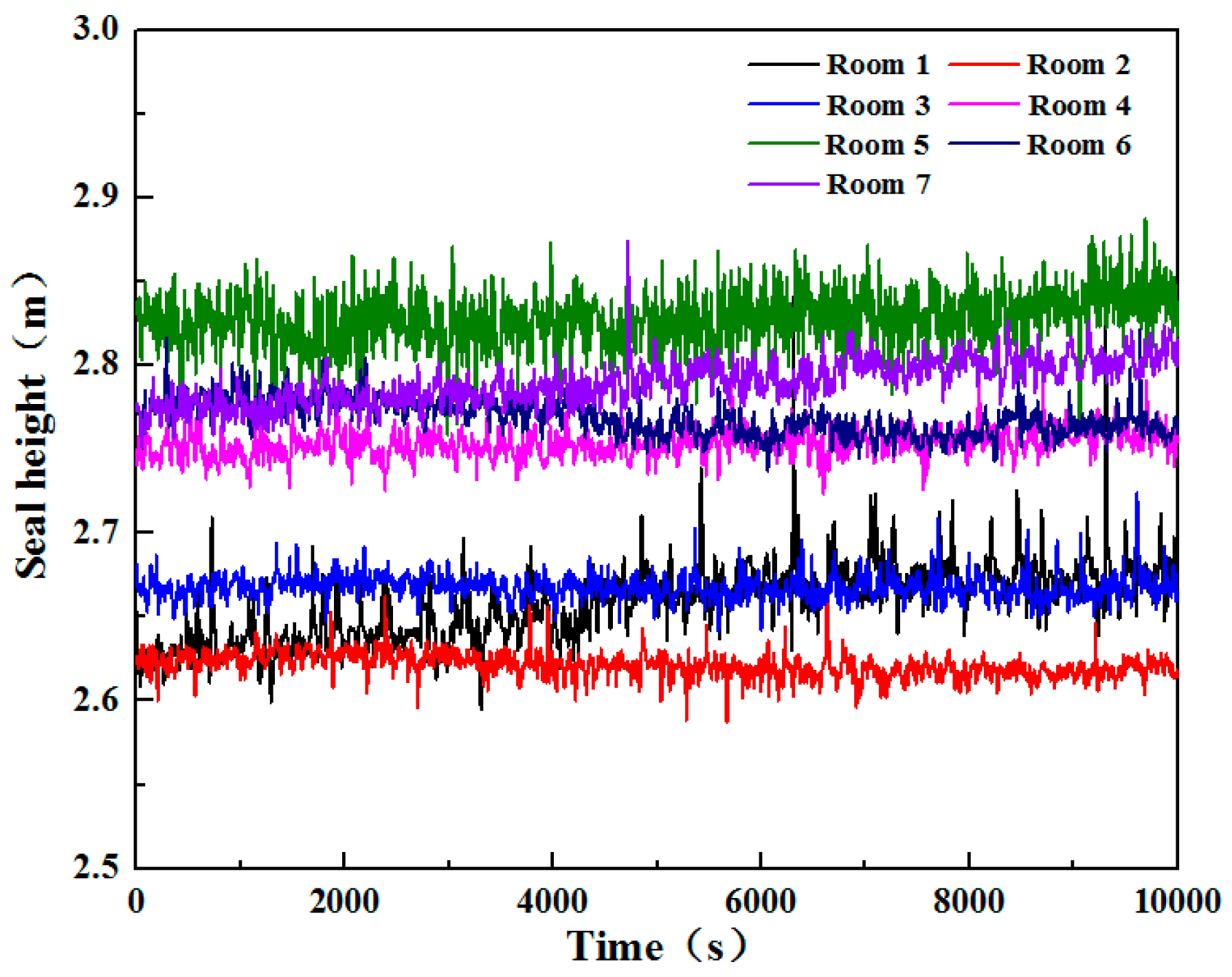
Figure 8.
Schematic diagram of the rocking motion of the system.

Figure 9.
Time history of heave motion of the system.

Figure 10.
Typical displacement power spectral density curve of heave motion.
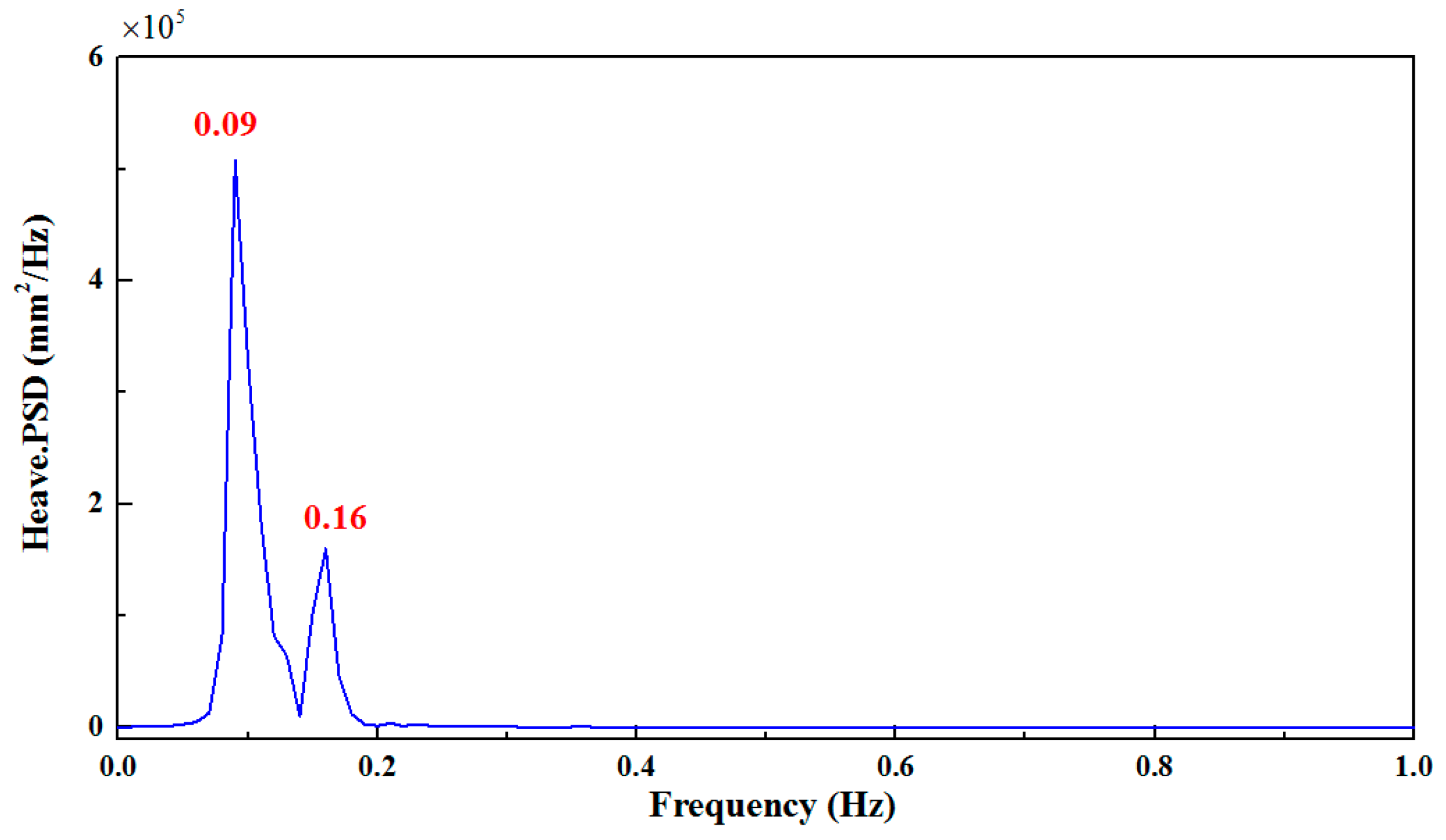
Figure 11.
Time history of X-direction motion displacement.
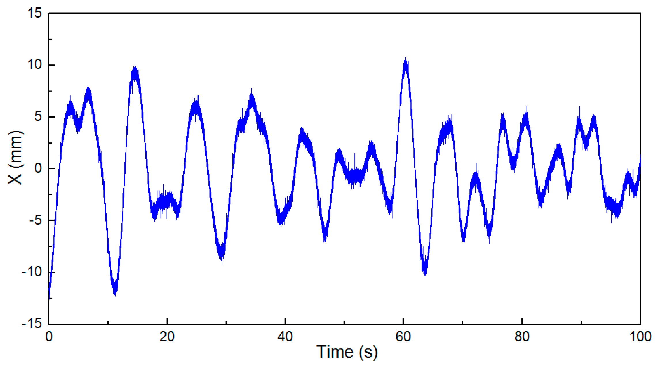
Figure 12.
Typical X-direction displacement power spectral density curve.

Figure 13.
Analytical and measured result of time history of heave displacement: (a) condition 1; (b) condition 2; (c) condition 3; (d) condition 4; (e) condition 5; (f) condition 6.
Figure 13.
Analytical and measured result of time history of heave displacement: (a) condition 1; (b) condition 2; (c) condition 3; (d) condition 4; (e) condition 5; (f) condition 6.

Figure 14.
Time history of motion at different vessel speeds: (a) heave; (b) pitch.

Figure 15.
The heave and pitch motion response as functions of vessel speed.

Figure 16.
Time history of motion at different vessel speeds: (a) heave; (b) pitch.

Figure 17.
The heave and pitch motion response as functions of vessel speed.

Figure 18.
Time history of motion at different wave heights: (a) heave; (b) pitch.

Figure 19.
The heave and pitch motion responses as functions of wind speed.
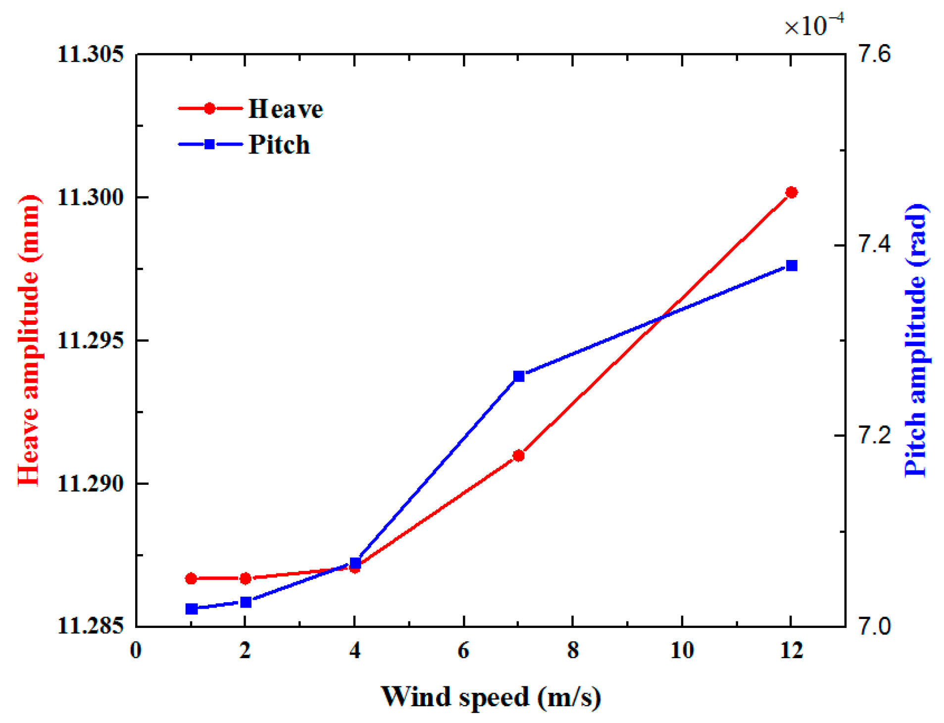
Figure 20.
Time history of motion at different wave angle: (a) heave; (b) pitch.

Figure 21.
The heave and pitch motion responses as functions of wave angle.

Figure 22.
The amplitude of motion response varies with each factor: (a) heave; (b) pitch.


Table 1.
Design parameters of the dedicated vessel and wind turbine structure.
| Vessel Property | Values | Wind Turbine Property | Values |
|---|---|---|---|
| Length | 103.2 m | Tower mass | 207.0 t |
| Molded depth | 9.0 m | Rotor-nacelle mass | 196.0 t |
| Molded breadth | 51.6 m | Tower height | 78.5 m |
| Designed draft | 6.0 m | Hub height | 90.0 m |
| Deck load | 20.0 t/m2 | Tower wall thickness | 48.0~22.0 mm |
| Tower diameter base, top | 4.3~3.2 m | ||
| Rotor diameter | 120.0 m |
Table 2.
Parameters in six selected conditions.
| Conditions | Speed (kn) | Wave Height (m) | Wind Speed (m/s) | Wave Angle (°) |
|---|---|---|---|---|
| Condition 1 | 5.0 | 0.2 | 1.0 | 0 |
| Condition 2 | 5.3 | 0.3 | 1.0 | 0 |
| Condition 3 | 3.5 | 0.4 | 1.3 | 0 |
| Condition 4 | 4.4 | 0.3 | 1.0 | 0 |
| Condition 5 | 5.5 | 0.6 | 1.3 | 0 |
| Condition 6 | 0.9 | 0.5 | 7.1 | 0 |
Table 3.
Heave displacements obtained from the analytical model and measured data.
| Conditions | Analytical Amplitude (mm) | Measured Amplitude (mm) | Amplitude Deviation (%) | Analytical RMS (mm) | Measured RMS (mm) | RMS Deviation (%) |
|---|---|---|---|---|---|---|
| Condition 1 | 18.321 | 17.451 | 4.99 | 9.128 | 8.550 | 6.76 |
| Condition 2 | 19.013 | 19.768 | 3.82 | 9.611 | 8.572 | 12.12 |
| Condition 3 | 21.504 | 24.725 | 13.03 | 10.376 | 9.467 | 9.60 |
| Condition 4 | 20.382 | 21.895 | 6.91 | 10.000 | 10.598 | 5.64 |
| Condition 5 | 23.872 | 23.343 | 2.23 | 12.004 | 12.061 | 0.47 |
| Condition 6 | 22.645 | 22.712 | 0.29 | 11.010 | 10.804 | 1.91 |
Table 4.
Heave Frequencies obtained from the analytical model and measured data.
| Conditions | Analytical (Hz) | Measured (Hz) | Deviation (%) |
|---|---|---|---|
| Condition 1 | 0.1087 | 0.1300 | 16.38 |
| Condition 2 | 0.1049 | 0.1200 | 12.58 |
| Condition 3 | 0.1179 | 0.1100 | 7.18 |
| Condition 4 | 0.1134 | 0.1000 | 13.40 |
| Condition 5 | 0.1022 | 0.1100 | 7.09 |
| Condition 6 | 0.1445 | 0.1500 | 3.67 |
Table 5.
The other influencing factors.
| Factors | Wave Height (m) | Wave Period (s) | Wind Speed (m/s) | Wave Angle (°) |
|---|---|---|---|---|
| Value | 0.3 | 9.05 | 7 | 0 |
Table 6.
The values of other influencing factors.
| Factors | Vessel Speed (kn) | Wave Period (s) | Wind Speed (m/s) | Wave Angle (°) |
|---|---|---|---|---|
| Value | 2 | 9.05 | 7 | 180 |
Table 7.
The values of other influencing factors.
| Factors | Vessel Speed (kn) | Wave Period (s) | Wave Height (m) | Wave Angle (°) |
|---|---|---|---|---|
| Value | 2 | 9.05 | 0.2 | 180 |
Table 8.
The values of other influencing factors.
| Factors | Vessel Speed (kn) | Wave Period (s) | Wave Height (m) | Wind Speed (m/s) |
|---|---|---|---|---|
| Value | 2 | 9.05 | 0.3 | 7 |
© 2019 by the authors. Licensee MDPI, Basel, Switzerland. This article is an open access article distributed under the terms and conditions of the Creative Commons Attribution (CC BY) license (http://creativecommons.org/licenses/by/4.0/).
Share and Cite
MDPI and ACS Style
Lian, J.; Jiang, J.; Dong, X.; Wang, H.; Zhou, H.; Wang, P. Coupled Motion Characteristics of Offshore Wind Turbines during the Integrated Transportation Process. Energies 2019, 12, 2023. https://doi.org/10.3390/en12102023
AMA Style
Lian J, Jiang J, Dong X, Wang H, Zhou H, Wang P. Coupled Motion Characteristics of Offshore Wind Turbines during the Integrated Transportation Process. Energies. 2019; 12(10):2023. https://doi.org/10.3390/en12102023
Chicago/Turabian StyleLian, Jijian, Junni Jiang, Xiaofeng Dong, Haijun Wang, Huan Zhou, and Pengwen Wang. 2019. "Coupled Motion Characteristics of Offshore Wind Turbines during the Integrated Transportation Process" Energies 12, no. 10: 2023. https://doi.org/10.3390/en12102023
Note that from the first issue of 2016, this journal uses article numbers instead of page numbers. See further details here.