A Practical Method for Speeding up the Cavitation Prediction in an Industrial Double-Suction Centrifugal Pump

Abstract

Researches have over the past few years have been applying optimization algorithms to quickly find optimum parameter combinations during cavitation optimization design. This method, although better than the traditional trial-and-error design method, consumes lots of computational resources, since it involves several numerical simulations to determine the critical cavitation point for each test case. As such, the Traditional method for NPSHr prediction was compared to a novel and alternative approach in an axially-split double-suction centrifugal pump. The independent and dependent variables are interchanged at the inlet and outlet boundary conditions, and an algorithm adapted to estimate the static pressure at the pump outlet. Experiments were conducted on an original size pump, and the two numerical procedures agreed very well with the hydraulic and cavitation results. For every flow condition, the time used by the computational resource to calculate the NPSHr for each method was recorded and compared. The total number of hours used by the new and alternative approach to estimate the NPSHr was reduced by 54.55% at 0.6 Q_d, 45.45% at 0.8 Q_d, 50% at 1.0 Q_d, and 44.44% at 1.2 Q_d respectively. This new method was demonstrated to be very efficient and robust for real engineering applications and can, therefore, be applied to reduce the computation time during the application of intelligent cavitation optimization methods in pump design.

1. Introduction

Among the various groups of pumps available, centrifugal pumps are the most popular and frequently used in the pump industry. In determining pump characteristics, however, two significant indexes of great concern have been used to improve the pump hydraulic performance characteristics and to minimize the cavitation. In addition, although the hydraulic performance of centrifugal pumps has generally undergone a series of advancements over the past years, two major problems have been consistent with its development. The first is flow instability problems primarily triggered by pressure pulsations [1], whereas the second has to do with cavitation, which occurs in situations where absolute pressure of the fluid drops lower than its saturated pressure within localized areas of the flow domain. Cavitation, which is generally a complex occurrence with an abrupt phase change, does not only erode the flow passage, but also induces flow blockage and violent pressure vibration, leading to noise, performance breakdown, and costly damage to hydraulic machineries [2]. The phenomenon has seen the introduction of a number of theories and concepts such as Net Positive Suction Head (NPSH), Thoma’s cavitation number, suction specific speed, etc, that evaluates a pump’s suction performance and operating conditions [3].

Over the years, a series of investigations have been carried out to understand the physics of cavitation inception; these investigations have always been geared towards understanding bubble growth and bubble dynamics and also in determining cavitation nuclei sources for the given flow situation. Other works have focused on the development of theoretical models to help predict cavitation occurrence. This includes some investigations on two-phase cavitating flow in pumps as well [4,5,6,7,8,9,10,11]. A detailed understanding of suction capability and pump cavitation has been summarized in Gulich’s technical book on centrifugal pumps [12]. The book thoroughly addresses impeller and diffuser cavitation; NPSH; and noise induced by cavitation, vibration and cavitation erosion. An understanding of the concept and theory of cavitation as well as cavitation types and bubble dynamics has also been given [13].

The desire to improve upon the cavitation performance has seen several efforts and alternative methods other than the traditional method for pump design, where model tests were employed as useful tools to obtain a pump’s performance. Over the last two decades, the development of numerical methods and the application of Computational Fluid Dynamics (CFD) to performance prediction for cavitating flows has seen remarkable progress in the pump industry [14]. In general, the industry practice for measuring the degree of cavitation has been by means of the NPSH. Zhang et al explained NSPHa (available NPSH) as the suction head available at the pump impeller inlet, whereas NPSHr (required) is the least suction head the pump needs so as to avoid excessive cavitation and pump performance degradation. This is usually referred to as NPSH3, since at a cavitation-induced head impairment ≥3% the cavitating pump will undergo significant cavitation, which eventually leads to head breakdown [9,15].

Traditionally, a series of CFD simulations are run during NPSHr predictions by gradually reducing the total inlet pressure at the impeller inlet until a 3% head drop is achieved. The corresponding NPSHr is then calculated for that point. For the boundary condition settings, the common practice has been to set the suction inlet to total pressure, while the boundary at the outlet is fixed to volume flow rate. Although this boundary set has been fruitfully implemented in numerical simulations with and without cavitation models [16,17,18,19,20], the choice of total inlet pressure is by guessing if there is no foreknowledge of the NPSHr range [21,22,23,24]. This approach usually requires about 10–15 independent simulations before a good accuracy is reached [15,16]. Moreover, this pure guessing game is likely to draw the simulation into severe cavitation conditions, which take far longer times to converge, especially in situations where transient simulations are required to acquire the necessary accuracy [14,25]. Engineers have over the years adopted optimization algorithms to improve performance by sampling a range of parameter combinations to find an optimal parameter combination that improves performance results. For cavitation optimization designs, the process involves the calculation of several test cases to determine the required Net Positive Suction Head (NPSHr) for each case which consumes a lot of computational time. A much more recent approach proposed by Ding et al [26] introduced a controllable and much more predictable simulation procedure where the traditional boundary sets were substituted by introducing a new set of boundary pairs which had the inlet being set to volume flow rate and an algorithm developed to estimate a good value for static pressure to be set for the outlet boundary. The procedure predicted NPSHr in three simulation steps for one flow rate in an industrial centrifugal pump. The new boundary pair used has been commonly used for non-cavitating conditions and proved to be numerically stable [14,26].

This paper investigates the NPSHr prediction methods and simulation time by employing both the traditional method of NPSHr prediction and an alternative approach where the independent and dependent variables are interchanged at the inlet and outlet boundary conditions in an industrial double suction centrifugal pump. It further draws a comparison between the two methods and provides a pathway for cavitation optimization in centrifugal pumps. The aim is to strengthen a theoretical reference that can be integrated to reduce computational costs during the application of optimization algorithms in cavitation optimization design of centrifugal pumps.

2. NPSHr Prediction Approach

2.1. The Traditional Method

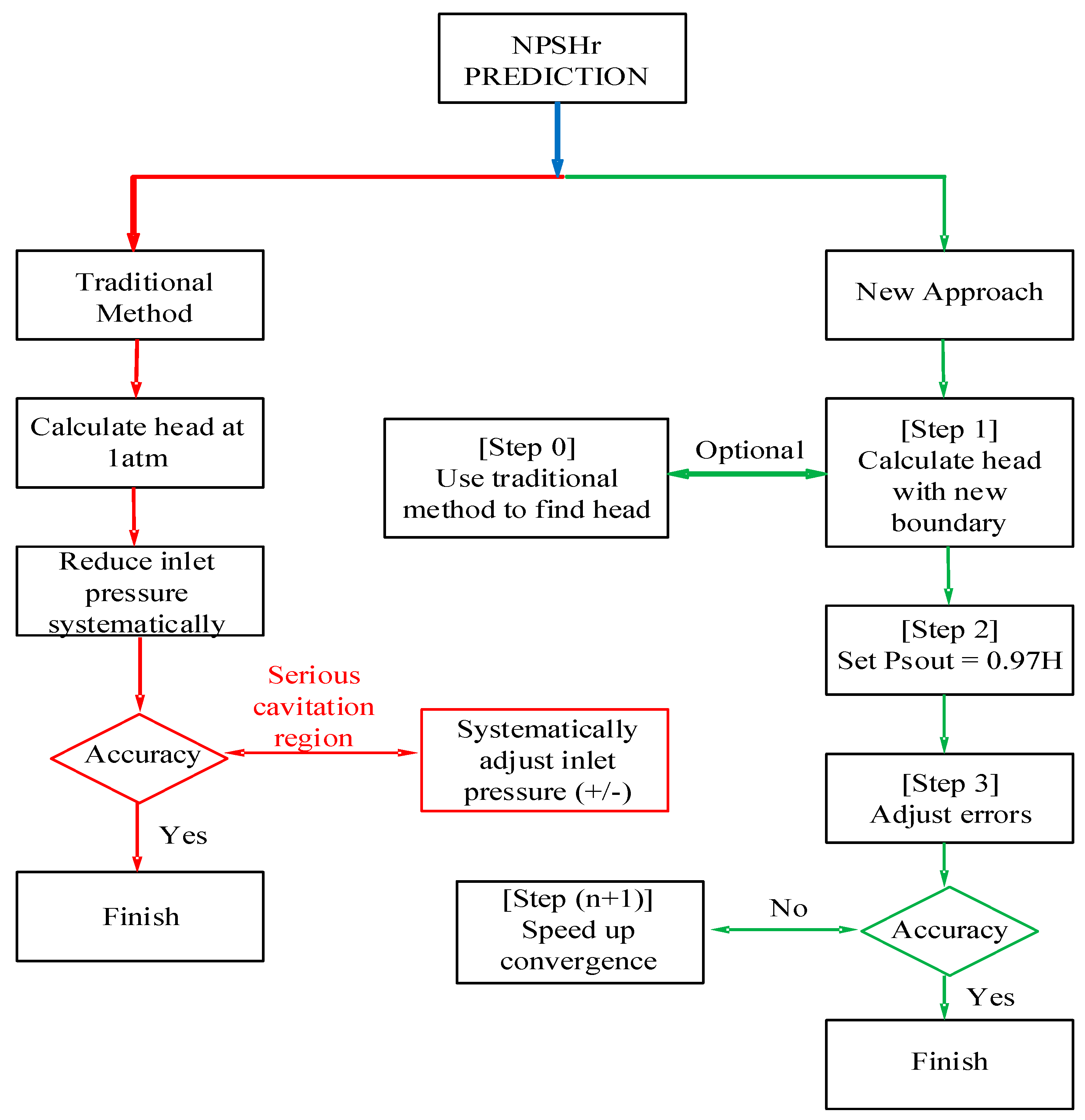
Figure 1 is a flowchart of the two prediction methods used in this study. The traditional method for NPSHr prediction has been widely used over the years. In this approach, the inlet boundary condition was set to total pressure while the outlet boundary condition was usually set to flow rate. For the initial step, the inlet pressure was set to 1atm to determine the pump head at no cavitation conditions. Next, the inlet pressure was decreased systematically and the NPSH available for each inlet pressure was calculated. The inlet pressure was systematically adjusted until the pump head dropped by 3%. The NPSH available at that point was calculated for the critical cavitation point. Since the inlet pressure at the critical cavitation point was not known, the selection of the inlet pressure was by speculation. The simulation therefore requires several steps to accurately predict the critical cavitation point. The bisection method was not applied to speed up the process. This is because the simulation usually enters the serious cavitation region where it takes a long time to converge. When the simulation enters the serious cavitation region, the inlet pressure has to be increased systematically to adjust. Thus, the gradual reduction of inlet pressure was used until the head drop approached 3% to avoid the serious cavitation region. The mathematical relation for NPSH is:

$$NPSH=\frac{p-p_v}{\rho g}+\frac{V_{in}{}^2}{2g}$$

(1)

Here, p is the static pressure at the inlet, V_in is the velocity at the inlet, p_v is the vapor pressure, ρ is the density, and g is the acceleration due to gravity [12].

2.2. Alternative NPSHr Prediction Procedure-Fundamental Algorithm

For a given flow rate condition, three key procedures are required to calculate the NPSHr. The approach used here is adapted from Ding et al [26]. There are, however, two other optional procedural steps (pre and post procedural) that can be applied discretionally where necessary.

Step 0 (optional): The first step is an optional procedure. It entails performing a quick simulation with the traditional boundary settings. This is to give an idea of the pump head for the flow rate being studied and can be skipped if the head is already known. The traditional boundary condition is as follows:

• Total pressure at inlet: $p_{tot-in}(0)=p_{tot-in}$
• Volumetric flow rate at outlet: $Q_{out}(0)=Q$

Step 1: In this step, the head of the pump is recalculated by introducing a new boundary pair to obtain a clear-cut reference point in predicting the 3% head drop. The boundary conditions for this step are as follows. The inlet is held fixed to the flow rate while an algorithm is used to estimate the static pressure at the pump outlet for the subsequent steps. The outlet static pressure, $p_{tot}$, is estimated as follows.

$$p_{out}(1)=H(0)+p_{tot-in}(0)-H_D(0)=p_{out}(0)$$

(2)

Step 2: The outlet static pressure is set to a fixed value of 97% of the pump head calculated from step 1. This step though below the 3% point is set to estimate a closely related head to the NPSHr. This step prevents the simulation from running into severe cavitation since the estimated NPSHa is not far from the cavitation point. The static pressure is estimated by the expression:

$$p_{out}(2)=0.97H_{100}-H_D(1)$$

(3)

Here, $p_{tot}(2)$ is used to express outlet static pressure for step 2; H₁₀₀, is the pump head at no head drop calculated from step 1, and H_D is the dynamic head calculated from step 1.

Step 3: The significance of this step is to correct the errors in the previous step by adjusting the outlet boundary condition. The predicted results are anticipated to be as near as possible to the NPSHr, the point where the head drops 3%. The procedure can be terminated here if the desired accuracy is achieved.

$$p_{out}(3)=0.97H_{100}+p_{tot-in}(2)-H_D(2)$$

(4)

Convergence Criteria

Where the desired accuracy is not achieved, a quadratic acceleration approach is adapted to fast-track the convergence rate.

$$a{n}_0{}^2+b{n}_0+c=0$$

(5)

where:

$$a=f-1$$

(6)

$$b=2n_1-2f{n}_2$$

(7)

$$c=f{n}_2{}^2-n_1{}^2$$

(8)

$$f=\frac{h_0-h_1}{h_0-h_2}$$

(9)

Solving the quadratic equation, the solution with the biggest value is

$$m=\frac{h_0-h_2}{{\left(n_0-n_2\right)}^2}$$

(10)

$$n_0=\frac{-b+\sqrt{b^2-4ac}}{2a}$$

(11)

The variables, n, and h, represent the NPSHa and pump head respectively. Here the simulation results from step 1 represents the value $h_0$, step 2 is $h_1$, and step 3 is $h_3$. Three simulation results are needed before the convergent criteria can be applied, and therefore the approach can only be applied after the third step. NPSHa for step 4 is denoted by $n_3$, and is expressed as:

$$n_3=n_0-\sqrt{\frac{0.03h_0}{m}}$$

(12)

Step (n + 1): This step serves as an acceleration technique that has the tendency to increase the convergence rate to the critical cavitation point. It is usually an optional step to draw the NPSHa closer to the prediction point in situations where the results from the previous step lies outside the predicted range.

$$p_{out}\left(n+1\right)=0.97H_{100}+n_3-H_D\left(n\right)$$

(13)

3. Description of Computational Domain

3.1. Computational Domain

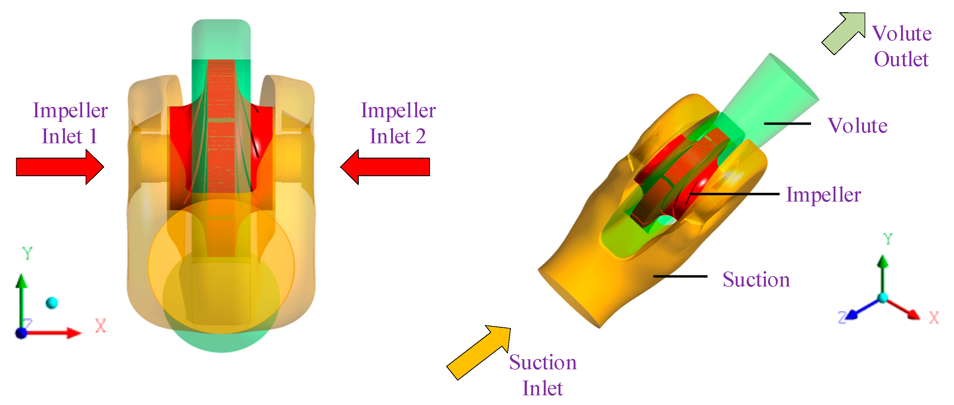
The 3D model for the computational domain was developed with PTC CREO Parametric 4.0. It was designed according to a specific speed n_s of 89.5 in Equation (14). The flow domain is divided into three sections. The impeller is a shrouded radial flow double-suction impeller with six twisted blades. The suction domain, which is semi-spiral in shape, has a single inlet and dual outlets. The flow on entering the suction unit split into two outlets to feed both eyes of the impeller. Each suction outlet has flow directing baffles introduced (suction tongue) to reduce the pre-swirl towards the impeller eye to reduce incidence losses at the impeller inlet. The pump has a single volute serving as the discharge and outlet unit. Figure 2 shows the pump model under investigation and the calculation domain, and

Table 1. Design specifications of model pump.

Design Parameters	Value
Flow rate, Qd (m3/s)	0.139
Head, H (m)	40
Rotational speed, N (r/min)	1480
Number of blades, z	6
Suction diameter, Ds (mm)	250
Impeller inlet diameter, D1 (mm)	192
Impeller outlet diameter, D2 (mm)	365
Delivery diameter, Dd (mm)	200
Efficiency, η	84
NPSHr (m)	3.5

presents the design specifics of the pump.

$$n_s=3.65\times \frac{N\times Q_d{}^{0.5}}{H^{0.75}}$$

(14)

where:

• N is rotating speed, rpm
• Q_d is flow rate at design point, m³/s
• H is head at design point, m

3.2. Computational Grid and Mesh Sensitivity

The flow passage for the tested pump was meshed with ANSYS ICEM 18.0 mesh tool. A hexahedral grid system was generated in the computational domain using O-type grids near the blade and H/C type grids near the leading with the trailing edge. The grid size and blocking method were used and the grids for the impeller and suction chamber were refined with large numbers for higher precision. A single blade passage was first meshed and transformed to six blades to make the full blade set. At the volute tongue region which is known to be very complex, the grids were concentrated. The leading and trailing edges of the impeller were also further refined to improve computational accuracy. The boundary layer and grid growth were set to ensure the density and thickness of the boundary layer mesh. An overview of the computational mesh is shown in Figure 3. To speed up the calculation time and still maintain accuracy in iterations, it is necessary to carry out a grid-independence analysis for the numerical simulation. Based on similar works [27,28,29,30], five independent high quality structural hexahedral meshes were built and a grid sensitivity analysis was executed. Simulations were performed at steady state at the design flow rate of Q_d = 0.139 m³/s to determine the mesh influence on pump head and efficiency.

For this simulation, the efficiency used is the hydraulic efficiency and the power is the mechanical power. To calculate for the performance indicators, the following mathematical relations were used [12]. The Head is expressed as:

$$H=\frac{p_{tot-out}-p_{tot-in}}{\rho g}$$

(15)

where $p_{tot-out}$ and $p_{tot-in}$ are total pressures at pump outlet and inlet respectively.

The pump hydraulic efficiency is expressed as:

$$\eta =\frac{\rho gHQ}{P_s}$$

(16)

here, H is the pump head, Q is the flow discharge, and P_S the shaft power.

Shaft power is expressed as:

$$P_s=T\omega$$

(17)

where T is the shaft torque and ω is the angular speed of the shaft.

The performance comparison for the five independent grids is presented in Figure 4. For Mesh I and II, the calculated performance indicators were lower than the design performance characteristics of the pump. The head, efficiency and power reached the design values when the mesh number was increased to 4,266,423 elements. For the subsequent mesh with higher grid numbers, the effects of the mesh density on the hydraulic performance remained fairly constant. Mesh III, Mesh IV and Mesh V were compared since they each met the design criteria for the pump. The effect of the higher mesh numbers on the pump performance was 0.025%, 0.01% and 0.075% for head, efficiency and power respectively. This suggested that numerical accuracy stabilized as the grid number increased to 4,266,423 elements. Mesh III was therefore used for the computations to reduce calculation load and computation time. The mesh density for the independent grids are presented in

Table 2. Grid cells of the various mesh.

Test Case	Number of Elements			Total Elements	Head (m)	Efficiency (%)	Power (kW)
	Impeller	Suction	Volute
Mesh I	542,256	1,938,727	397,260	2,878,243	33.21	67.50	55,298.14
Mesh II	1,343,355	1,938,727	397,260	3,679,342	38.40	76.44	59,525.58
Mesh III	1,199,880	1,938,727	1,127,816	4,266,423	40.55	88.04	62,753.44
Mesh IV	1,786,536	1,938,727	1,232,905	4,958,168	40.54	88.05	62,867.96
Mesh V	1,786,536	1,938,727	2,122,494	5,847,757	40.56	88.04	63,086.63

.

3.3. Governing Equations

In simulating cavitation flow, the fluid model is assumed to be homogeneous since it is a compressible mixture of liquid and vapor. A two-phase mixture model and cavitation model are therefore a necessity. The continuity equation, which is the basic equation governing two-phase flow, is adopted from the Navier-Stokes equations [31], which is time-dependent and is given as

$$\frac{\partial {\rho }_m}{\partial t}+\frac{\partial }{\partial x_j}\left({\rho }_m{u}_j\right)=0$$

(18)

$$\frac{\partial \left({\rho }_m{u}_i{u}_j\right)}{\partial x_j}+\frac{\partial }{\partial t}\left({\rho }_m{u}_i\right)=\frac{\partial p}{d{x}_i}+\frac{\partial }{d{x}_j}\left[\left(\mu +{\mu }_t\right)\left(\frac{\partial u_i}{\partial x_j}+\frac{\partial u_j}{\partial x_i}+\frac{2}{3}\frac{\partial u_k}{\partial x_k}{\delta }_{ij}\right)\right]$$

(19)

Density and dynamic viscosity mixtures are represented by ρ and μ respectively. Velocity is denoted by u, p is the pressure, and turbulent viscosity is μ_t. Variables i and j are axis directions. The turbulence model chosen was SST k–ω because it exhibits a combined advantage of both the k–ω and k–ε turbulence models [32,33]. Transport equations for k and ω are expressed follows.

$$\frac{\partial \left({\rho }_{m}k\right)}{\partial t}+\frac{\partial \left({\rho }_m{u}_{j}k\right)}{\partial x_j}=P_k-{\beta }^{*}{\rho }_{m}k\omega +\frac{\partial }{d{x}_j}\left[\left(\mu +\frac{{\mu }_t}{{\sigma }_{k3}}\right)\frac{\partial k}{\partial x_j}\right]$$

(20)

$$\begin{array}{l}\frac{\partial \left({\rho }_m\omega \right)}{\partial t}+\frac{\partial \left({\rho }_m{u}_j\omega \right)}{\partial x_j}=\\ a_3\frac{\omega }{k}{P}_k-{\beta }_3{\rho }_m{\omega }^2+\frac{\partial }{d{x}_j}\left[\left(\mu +\frac{{\mu }_t}{{\sigma }_{\varpi 3}}\right)\frac{\partial \omega }{\partial x_j}\right]+2\left(1-F_1\right){\rho }_m\frac{1}{\omega {\sigma }_{\omega 2}}\frac{\partial k}{\partial x_j}\frac{\partial \omega }{\partial x_j}\end{array}$$

(21)

$$P_k={\mu }_t\left(\frac{\partial u_i}{\partial x_j}+\frac{\partial u_j}{\partial x_i}\right)\frac{\partial u_i}{\partial x_j}-\frac{2}{3}\left({\rho }_{m}k+3u_t\frac{\partial u_k}{\partial x_k}\right)\frac{\partial u_k}{d{x}_k}$$

(22)

The turbulence viscosity equations are:

$${\mu }_t=\frac{{\rho }_m{a}_{1}k}{\max \left(a_1\omega ,{\mathrm{SF}}^2\right)}$$

(23)

$$s=\sqrt{\left(\frac{\partial u_i}{\partial x_j}+\frac{\partial u_j}{\partial x_i}\right)}\frac{\partial u_i}{\partial x_j}$$

(24)

$$F_1=\tanh \left\{{\left\{\min \left[\max \left(\frac{\sqrt{k}}{{\beta }^{*}\omega y},\frac{500v}{y^2\omega }\right),\frac{4{\rho }_{m}k}{C{D}_{k\omega }{\sigma }_{\omega 2}{y}^2}\right]\right\}}^4\right\}$$

(25)

$$C{D}_{k\omega }=\max \left(2{\rho }_m\frac{1}{{\sigma }_{\omega 2}}\frac{\partial k}{\partial x_j}\frac{\partial w}{\partial x_j},1.0E^{-10}\right)$$

(26)

$$F_2=\tanh \left\{{\left[\max \left(2\frac{\sqrt{k}}{{\beta }^{*}\omega y},\frac{500v}{y^2\omega }\right)\right]}^2\right\}$$

(27)

The cavitation model used is the mass transport equation deduced from Rayleigh-Plesset’s equation. Transport equation for bubble formation and collapse is expressed as:

$$\frac{\partial \left({\rho }_v{\alpha }_v\right)}{{\partial }_t}+\frac{\partial }{\partial x_j}\left({\rho }_v{\alpha }_v{u}_j\right)=\dot{m}={\dot{m}}^{+}-{\dot{m}}^{-}$$

(28)

$$m^{+}=C_{vap}\frac{3r_g\left(1-{\alpha }_v\right){\rho }_v}{R_b}\sqrt{\frac{2}{3}\frac{\max \left(p_v-p,0\right)}{{\rho }_l}}$$

(29)

$$m^{-}=C_{cond}\frac{3{\alpha }_v{\rho }_v}{R_b}\sqrt{\frac{2}{3}\frac{\max \left(p-p_v,0\right)}{{\rho }_l}}$$

(30)

Whereby, α_v denotes the vapor fraction and m⁺ and m⁻ stand for mass transfer terminology for evaporation and condensation respectively. The coefficients for condensation and evaporation phases are represented as C_cond and C_vap. r_g is the nucleation site volume fraction, R_b is the bubble radius, ρ_v is the vapor density, ρ_l, the liquid density and p_v, which is also the saturation pressure. Standardized values according to the literature are: C_vap = 50, C_cond = 0.01, r_g = 5 × 10⁻⁴, R_b = 10⁻⁶ m, ρ_v = 0.554 kg/m³, ρ_l = 1000 kg/m³ and p_v = 3169 Pa [34,35]. The governing equations used are the default equations present in the ANSYS software package used.

3.4. Numerical Simulation Setup

Three-dimensional Reynolds-Averaged Navier Stokes (3-D RANS) equation for a fully developed flow was solved using the commercial CFD package ANSYS CFX. Water at room temperature was selected as the working fluid for the homogeneous fluid model and the reference pressure was set to 0 atm. An isothermal heat transfer rate was selected to render the system in thermal equilibrium with its surroundings at 25 °C. The Shear Stress Transport (SST k-ω) turbulence model was applied since it has a combined advantage of both k–ω and k–ε turbulence models. The advantages of the k-ω model can be extended by the automatic wall treatment to ensure the accuracy of the pressure gradient regardless of the distance to the nearest wall [32,33]. The direction of the flow was set normal to the boundary condition. In addition, a standard no-slip condition was applied and the wall roughness was smooth for all flow domains. Due to additional effects in the viscous sublayer, an automatic near-wall treatment was applied. A medium turbulence intensity level of 5% was chosen at the pump inlet. This is the default setting in the CFX–Pre setup and has been applied on centrifugal pumps with similar characteristics [14,36]. To guarantee consistency, convergence and accuracy during the simulations, a high-resolution upwind scheme was employed to solve both steady and unsteady equations. This adaptive numeric scheme locally adjusts the discretization to be as close to second-order as possible, while ensuring the physical boundedness of the solution. A frozen rotor with a pitch angle of 360° was selected. The frozen-rotor condition was used as the frame change model. The method of frozen-rotor transforms a rotating domain into a stationary domain depending on the position of the initial grid and considers it appropriately for all rotating domains. The advantage of this method is that it uses less computer resources than other frame change models, making it suitable and robust. For no cavitation conditions, pressure opening and flowrate boundary conditions were specified at the inlet and outlet. The Zwart-Gerber-Belamri (ZGB) model was used for cavitation simulations. Cavitation simulations were first performed under steady state with boundary conditions specified as static pressure for the outlet and mass flowrate at the inlet. The volume fraction of water (1-α) was set to (1), whereas the vapor volume fraction, α, set to (0) at the inlet of the pump. Steady state iterations were set to a maximum of 700 for no cavitation conditions and up to 3000 for cavitation conditions. Iterations, however, converged when maximum residual values were less than or equal to 10⁻⁵, and this occurs when the flow has reached its stable periodicity. The head, efficiency and power at each operating condition were calculated by averaging iterations of the last 100 head values of the steady-state simulations.

3.5. Test Setup to Validate Numerical Method

The pump performance tests were done at the open test rig system. The test rig schematics can be seen in Figure 5. The test system and the tested pump are shown in Figure 6. An air bleed valve was installed at the highest point of the volute to get rid of entrained air in the pump. During operation of the pump, the air bleed valve also supplies water to the mechanical seals to cool them. The diameter of the suction pipe is 250 mm and the diameter of the outlet pipe is 200 mm. The flow rate was measured with an electromagnetic flowmeter with uncertainty 0.07%, and it is installed in the outlet pipe line, 2500 mm from the pump. The fluid pressure at suction and discharge points was measured with high-precision pressure transmitters with uncertainty of 0.5%, which were installed directly in the pipeline. The pressure transmitter at the suction end is installed at 500 mm from the pump, whereas the outlet transmitter is installed at 1000 mm.

Before startup of the pump, the discharge valves were shut and the pump was primed while paying attention to the air bleed valve to discharge the air in the pump. The motor was started until it reached its rated speed of 1480 rpm. The discharge valve was then opened and gradually adjusted to the desired performance condition. The inlet and outlet pressures and the flow rate were recorded. Next, the outlet valve was systematically adjusted to the desired flow rate and the readings were taken. At each step, the motor speed was adjusted to maintain 1480 rpm. For the cavitation tests, the inlet valve was first closed a little to reduce the inlet pressure to the desired value. Then, the outlet valve was systematically adjusted to maintain a constant flow rate. Measurements were then taken and the procedure repeated each time by further closing the inlet valve to reduce the inlet pressure until the NPSHr at the reference flow rate was achieved. Cavitation experiments were performed for three flow conditions. Afterwards, the discharge valve was gradually closed and the power was cut to shut down the pump.

4. Discussion of Results

4.1. Numerical Model Validation

The numerical simulation did not take into account the mechanical and volumetric losses during the simulation, hence the efficiency calculated from the simulation results is the hydraulic efficiency only. In order to be able to compare the simulation results with the experimental results, the overall efficiency of the pump, which is a product of the hydraulic efficiency ${\eta }_h$, the mechanical efficiency ${\eta }_m$, and the volumetric efficiency ${\eta }_v$, has to be considered. This is because the during the experiments, mechanical losses and volumetric loses occur. Thus, following the examples from Refs. [14,37], the efficiency obtained from the simulation is further processed to include the mechanical and volumetric losses, before comparing with the test results. The mechanical efficiency is expressed as:

$${\eta }_m=1-0.07\frac{1}{{\left(\raisebox{1ex}{$n_s$}\!\left/ \!\raisebox{-1ex}{$100$}\right.\right)}^{\raisebox{1ex}{$7$}\!\left/ \!\raisebox{-1ex}{$6$}\right.}}$$

(31)

The Volumetric efficiency is expressed as:

$${\eta }_v=\frac{1}{1+{\left(0.68n_s\right)}^{\raisebox{1ex}{$-2$}\!\left/ \!\raisebox{-1ex}{$3$}\right.}}$$

(32)

The relationship between the efficiencies is expressed as:

$$\mathit{\eta }={\mathit{\eta }}_h{\mathit{\eta }}_m{\mathit{\eta }}_v$$

(33)

The pump motor is a YE2-280M-4 (Shanxi Electric Motor Manufacturing Co., Ltd., Taiyuan, China) with a rated power of 90 kW, and the connection type is delta connection. The voltage is 380 V. To determine the pump efficiency from the experiments, Equation (16) was used. To calculate for shaft power, the electrical output of the pump was used, and the relation used to calculate is as follows.

$$P_s=1.732\times \cos \phi \times I\times V\times {\eta }_{motor}\times {\eta }_{coupling}$$

(34)

where P_s is the shaft power, I is the current, V is the voltage, $\cos \phi =0.87$ is the Power Factor for the alternating current, while the electric motor efficiency is ${\eta }_{motor}=93.9\%$ and ${\eta }_{coupling}=98.7\%$ is the shaft coupling efficiency.

The measured quantities have for the efficiency have been presented in

Table 3. Results from the experiments.

Q (m3/s)	H (m)	Current (A)	Ps (kW)	Efficiency (%)
0	48.217	63.083	33.477	0
0.027	47.6	69.723	37.001	34.653
0.056	47.318	83.528	44.327	58.387
0.085	46.81	99.661	52.888	73.48
0.097	46.18	106.468	56.501	77.754
0.111	44.994	112.297	59.595	82.251
0.127	43.642	120.575	63.987	84.993
0.133	42.85	123.47	65.523	85.182
0.139	41.833	126.266	67.007	85.203
0.144	41.49	128.646	68.27	86.63
0.146	40.927	129.234	68.582	85.334
0.153	39.895	132.753	70.45	85.242
0.167	37.758	137.015	72.711	85.005
0.182	34.796	141.394	75.035	82.81
0.193	31.232	144.543	76.706	76.909
0.198	28.955	145.701	77.321	72.562

. Due to the difficulty in the repeatability of the experiments, the experiment was performed once. Type B evaluation was therefore used to estimate the systematic uncertainty using the calibration uncertainties of the sensors. The standard uncertainty for Type B evaluation [38] is expressed as:

$$E=\pm \frac{a}{\sqrt{3}}$$

(35)

$$E_{eff}=\pm \sqrt{E_{flowmeter}{}^2+E_{p-inlet}{}^2+E_{p-outlet}{}^2}$$

(36)

where E is the estimated standard uncertainty, and a is the calibration uncertainty of the sensor, $E_{eff}$ is systematic uncertainty of the pump efficiency, $E_{flowmeter}$ is the systematic uncertainty of the measured flow rate whereas the uncertainty of the pressure signals measured at the inlet and outlet are $E_{p-inlet}$ and $E_{p-outlet}$ respectively. The flowmeter has an uncertainty of 0.07%, thus from Equation (35) $E_{flowmeter}=\pm 0.04\%$. The pressure transmitters has an uncertainty 0.5%, and therefore $E_{p-inlet}=\pm 0.289\%$ and $E_{p-outlet}=\pm 0.289\%$. Using Equation (36), the systematic uncertainty of the efficiency is $u_{eff}=\pm 0.411\%$ which is accepted for engineering applications.

Numerical calculation for the non-cavitating pump was performed for different flow conditions, thus 0.4Q_d∓1.2Q_d. Figure 7 presents a comparison of performance characteristics for the two boundary pairs. The least deviation in numerical head was 0.008%, and this occurred at the design point, whereas a maximum deviation of 0.239% occurred at the deep part load. The numerical efficiency recorded a minimum deviation of 0.037% at the design point, meanwhile the maximum deviation was 0.262%. Looking at the deviation in numerical results for the two boundary pairs, either boundary pair can be used for the experimental validation since the difference is very minimal.

Computational results from the new boundary pair were matched with the experiments in Figure 8a. The pump head dropped gradually as the flow rate was increased, and the trends between the numerical and experimental heads were quite similar. The experimental head was however higher than the numerical head whereas the efficiency from the test results was lower than the calculate efficiency. The experimental head at the BEP was 41.49 m, and the corresponding efficiency was 86.63% at a flow rate of 0.144 m³/s, whereas the BEP for the numerical predictions occurred at head 40.24 m and efficiency 88.39 % at the design flow condition of 0.139 m³/s. The relative errors at the BEP were 3.01% and 2.03% respectively. The experimental head at the design point was 41.83 m and efficiency 85.20%. Figure 8b is a comparison of the mechanical power from the steady (RANS) and unsteady (URANS) simulations results. The mechanical power from the simulations were computed using Equation (17), and the power from the experiments was computed using Equation (34). The results from the steady and unsteady simulations were very similar. Therefore, the steady-state simulations could be used to predict similar results. Overall, the agreement between the results from the experiments and the simulation was very good, and this affirmed the reliability of the numerical approach.

4.2. Cavitation Performance Characteristics

A comparison of the cavitation characteristics between the two boundary pairs and the experimental results is shown in Figure 9. For the traditional method, the NPSHr was recorded at 2.592 m, which corresponded to a 2.9% head drop. This is shown in Figure 9a. When the boundaries were switched, the calculated NPSHr was 2.532m at a corresponding head drop of 3.20%. The experimental NPSHr for the design flow rate was calculated as 2.739 m, and the deviation from the experimental results was 5.37% for the traditional boundary pair and 7.56% for the new boundary pair. Although there is a 2.31% deviation in NPSHr between the numerical methods, the NPSHr for the traditional method corresponds to 2.9% head drop whereas the NPSHr for the new boundary pair corresponds to 3.20% of the head drop. The deviation is, however, expected to reduce when the predicted NPSHr value obtained is calculated exactly at respective 3% head drop point. The critical NPSH curves at different flow rates for the numerical and experimental results are compared in Figure 9b. At 0.6Q_d the suction performance of the experiment was lower than the numerical results. For all other flow conditions, the numerical results were lower than the experimental results. The deviations were minimal and therefore the two boundary condition sets agreed well with the experimental results to establish the suitability of both numerical methods for simulating cavitation flow.

4.3. Comparing the NPSHr Prediction Steps

Both the traditional and novel NPSHr prediction approaches were applied using steady-state computations to determine the NPSHr of the pump. The two different boundary pairs were used to calculate the NPSHr over the range of 0.6Q_d–1.2Q_d flow rates. Also, during the simulation process, the initial results of the previous simulation were used to begin every new simulation. The total hours used by the computational resource to calculate the NPSHr was referred to as the simulation time. Therefore, for every flow condition, the number of hours used by the computational resource in each simulation step was added, and the total number of hours used for the methods were compared. The computational resource used is Intel Xeon CPU E5-2687W v3 @3.10GHz, with 20 processor cores and 64 GB RAM. For each simulation, eight processor cores were used.

Table 4. Total number of hours during simulation.

Flowrate	Trad (Steps)	New (Steps)	%
0.6Qd	60.3 hrs (11)	32.9 hrs (5)	54.55
0.8Qd	48.3 hrs (11)	22 hrs (6)	45.45
1.0Qd	42.3 hrs (10)	21.2 hrs (5)	50
1.2Qd	42 hrs (9)	16.6 hrs (5)	44.44

. provides details of how the simulation time was calculated.

Figure 10a–c compares the two numerical methods used in the NPSH prediction for design and off-design flow conditions. For the traditional method, the gradual reduction method was used to predict the NPSHr whereas the novel method used a combination of a new boundary pair and an algorithm to estimate the corresponding static pressure at the pump outlet when the head drops by 3%. At 0.6Q_d, the traditional method used 11 calculating steps to predict a 3.12% head drop while the new approach predicted a 3.20% head drop after 5 calculation steps. This is shown in Figure 10a. The NPSHr prediction steps at 0.8Q_d are shown in Figure 10b. At 0.8Q_d, the NPSHr was predicted in 11 simulations using the traditional method. The new approach, however, used six steps to predict the critical cavitation point. This indicates that the new method reduced the calculation time by 45.45%. At the design point, the prediction was achieved with five simulations when the new method was applied. The traditional method for the design point calculated the critical cavitation point in 10 simulations. There was a 50% reduction in the number of simulations at the design point, and the comparison of the two methods can be seen in Figure 9a. When the flow was increased to 1.2Q_d, the new method predicted the NPSHr within five calculation steps while the traditional method required nine simulations to reach the critical cavitation point. At overload condition, the new method reduced the calculation time by 44.44%. Figure 10c is a comparison of the prediction methods at overload condition.

Generally, the new method reduced the simulation time significantly. From the steady-state cavitation simulations, the new approach was faster in predicting the critical cavitation point. It must also be noted that this approach does not give an account of the full cavitation curve that is from no cavitation, inception, and critical point to breakdown at large cavitation. It only focuses on the NPSHr and applies the algorithm to predict it. To determine cavitation inception, the same procedure can be followed; however, for inception, the outlet static pressure must be set to correspond to 1% drop in pump head.

4.4. Vapor-Phase Volume Fraction Distribution

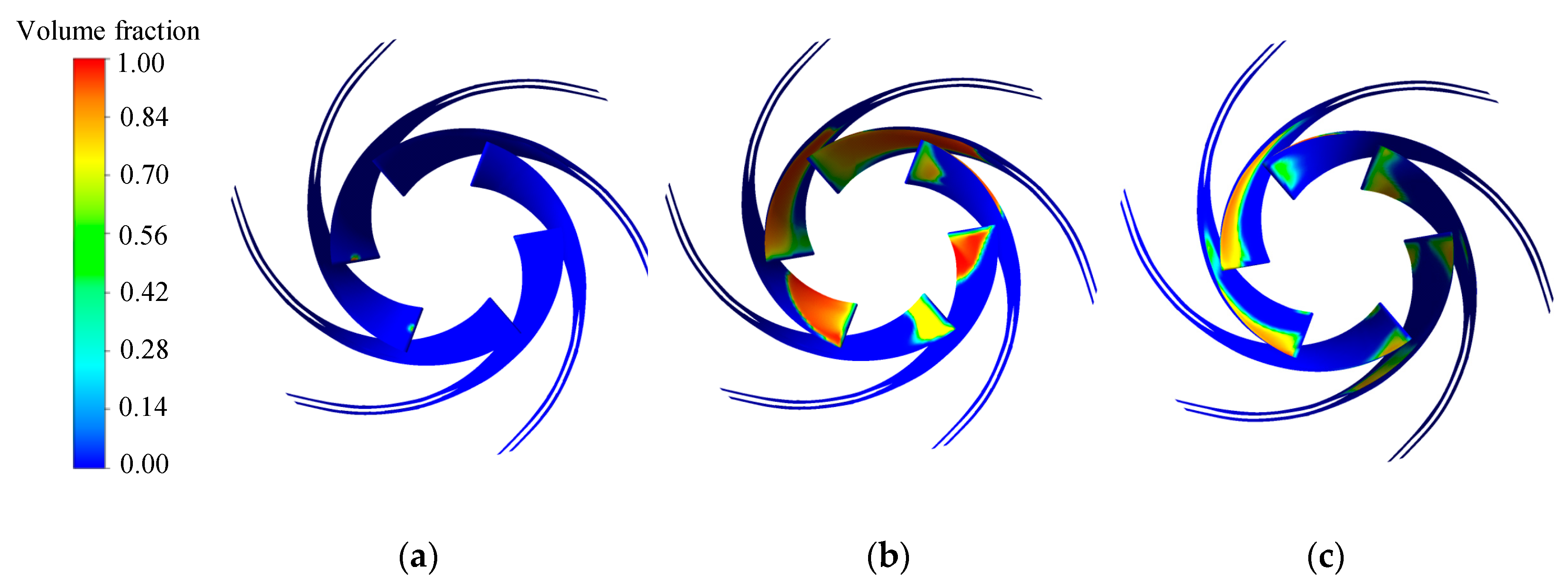
The vapor volume fraction was investigated to demonstrate the prediction ability of the new cavitation prediction method. The attached cavities were investigated for 0% head drop, 1% head drop, and 3% head drop, that is for the head at no cavitation (NPSH_0%), for 1% drop in pump head (NPSH_1%), and 3% drop in head (NPSH_3%) respectively. In the range of NPSH_0% and NPSH_1%, the rate of head drop was quite slow, making it difficult to also determine the exact conditions for which the head actually started dropping to critical cavitation level. Visualization of the attached cavity was therefore observed by CFD.

Figure 11, Figure 12, Figure 13 and Figure 14 show cavity development in the impeller and suction units of the flow domain. Isosurfaces were used to describe the cavity shape developed within the flow domains. For the respective NPSHa conditions of NPSH_0%, NPSH_1%, and NPSH_3%, all attached cavities above values of 5% vapor volume in the flow domain were visually observed. Figure 11 shows the vapor volume fraction distribution in the impeller at 0.6Q_d. The head was fairly constant at between NPSHa = 10.06 m and 2.35 m. At the head detection stage, a few cavities could be seen at the left corner of the leading edge for three blades. As the NPSHa value further reduced, a series of vapors started forming at the leading edge, and spreading towards the suction side. When NPSHa reached 2.35 m (NPSH_1%) and 2.16 m (NPSH_3%), the cavity volume increased considerably and extended to the pressure side. Further reduction in pressure at the impeller inlet resulted in bubble blockage at the blade channels and the head plunged into breakdown. The vapor burst quickly when the bubbles reached a higher pressure region, towards the impeller outlet. The trend was generally the same for the design and overload conditions, which can be seen in Figure 12 and Figure 13 respectively. Overall, it can be concluded that any decrease in the NPSHa resulted in a subsequent increase of cavitation which increasingly spread from the impeller inlet towards the outlet. The cavity concentration was along the blade suction surface because there was low pressure at the suction surfaces. The attached cavity at the critical cavitation point in the suction domain is shown in Figure 14. At 0.6Q_d, cavity formation was very minimal and formed on little portions of the wear rings in the suction. At the design and overload conditions of 1.0Q_d and 1.2Q_d, bubbles formed on a greater portion of the suction ring. The left half of the suction did not record any bubble formation for both the design and overload conditions. The dynamic-static coupling between the impeller and volute tongue may have caused the volume fraction distribution to be non-axisymmetric in the blade channels and suction unit. For all flow conditions investigated, there were no traces of cavities in the volute for vapor volume fraction values above 5%.

5. Conclusions

To determine a faster method for NPSHr prediction, an axially-split industrial double-suction centrifugal pump was numerically investigated using two numerical methods to predict the NPSHr of the pump. The two methods were presented and explained in detail. During the numerical investigations, a series of steady state simulations were carried out using the SST (k-ω) turbulence model and the ZGB cavitation model. For the design point, there was a deviation of 0.0076% and 0.0373% in the numerical head and efficiency when the two methods were compared. To validate the numerical models used, experiments were carried out in an open test rig system. The deviation was very minimal and both numerical methods were in good agreement when subjected to experimental validation to demonstrate their suitability for hydraulic and cavitation flow simulations. For every flow condition, the time used by the computational resource to calculate the NPSHr for each method was recorded and compared. The total number of hours used by the new and alternative approach to estimate the NPSHr was reduced by by 54.55% at 0.6 Q_d, 45.45% at 0.8 Q_d, 50% at 1.0 Q_d, and 44.44% at 1.2 Q_d respectively. Also, the vapor volume fraction was clearly revealed, and there were some attached cavities around the suction rings at NPSH_3%. From the results, it can be concluded that the alternative approach can be applied to quickly find the NPSHr during the application of optimization algorithms in the cavitation optimization design process for centrifugal pumps.

References

- Pei, J.; Wang, W.; Pavesi, G.; Osman, M.K.; Meng, F. Experimental Investigation of the Nonlinear Pressure Fluctuations in a Residual Heat Removal Pump. Ann. Nucl. Energy 2019, 131, 63–79. [Google Scholar] [CrossRef]
- Miyabe, M.; Maeda, H. Numerical Prediction of Pump Performance Drop and Erosion Area Due to Cavitation in a Double-Suction Centrifugal Feedpump. In Proceedings of the ASME-JSME-KSME 2011 Joint Fluids Engineering Conference, Hamamatsu, Japan, 24–29 July 2011. [Google Scholar]
- Luo, X.W.; Ji, B.; Tsujimoto, Y. A review of cavitation in hydraulic machinery. J. Hydrodyn. 2016, 28, 335–358. [Google Scholar] [CrossRef]
- Plesset, M.S. The Dynamics of Cavitation Bubbles. J. Appl. Mech. 1949, 16, 277–282. [Google Scholar] [CrossRef]
- Arndt, R.E.; George, W.K. Pressure Fields and Cavitation in Turbulent Shear Flows; National Academy of Sciences: Washington, DC, USA, 1979. [Google Scholar]
- Hirschi, R.; Dupont, P.; Avellan, F.; Favre, J.-N.; Guelich, J.-F.; Parkinson, E. Centrifugal Pump Performance Drop Due to Leading Edge Cavitation: Numerical Predictions Compared With Model Tests. J. Fluids Eng. 1998, 120, 705–711. [Google Scholar] [CrossRef]
- Dupont, P.; Casartelli, E. Numerical Prediction of the Cavitation in Pumps. In Proceedings of the ASME 2002 Joint US-European Fluids Engineering Division Conference, Montreal, QC, Canada, 14–18 July 2002. [Google Scholar]
- Biluš, I.; Predin, A. Numerical and experimental approach to cavitation surge obstruction in water pump. Int. J. Numer. Methods Heat Fluid Flow 2009, 19, 818–834. [Google Scholar] [CrossRef]
- Schiavello, B.; Visser, F.C. Pump Cavitation: Various Npshr Criteria, Npsha Margins, Impeller Life Expectancy. In Proceedings of the 25th International Pump Users Symposium, Houston, TX, USA, 23–26 February 2009. [Google Scholar]
- Liu, H.-L.; Wang, J.; Wang, Y.; Zhang, H.; Huang, H. Influence of the empirical coefficients of cavitation model on predicting cavitating flow in the centrifugal pump. Int. J. Nav. Arch. Ocean Eng. 2014, 6, 119–131. [Google Scholar] [CrossRef] [Green Version]
- Fu, Q.; Zhang, F.; Zhu, R.; He, B. A systematic investigation on flow characteristics of impeller passage in a nuclear centrifugal pump under cavitation state. Ann. Nucl. Energy 2016, 97, 190–197. [Google Scholar] [CrossRef]
- Gülich, J.F. Centrifugal Pumps; Springer Science & Business Media: Berlin, Germany, 2010. [Google Scholar]
- Franc, J.-P.; Michel, J.-M. Fundamentals of Cavitation; Chapter 12: Cavitation Erosion; Springer Science & Business Media: Berlin, Germany, 2006; Volume 76. [Google Scholar]
- Tang, X.; Zou, M.; Wang, F.; Li, X.; Shi, X. Comprehensive Numerical Investigations of Unsteady Internal Flows and Cavitation Characteristics in Double-Suction Centrifugal Pump. Math. Probl. Eng. 2017, 2017, 1–13. [Google Scholar] [CrossRef]
- Zhang, F.; Yuan, S.; Fu, Q.; Pei, J.; Böhle, M.; Jiang, X. Cavitation-Induced Unsteady Flow Characteristics in the First Stage of a Centrifugal Charging Pump. J. Fluids Eng. 2017, 139, 011303. [Google Scholar] [CrossRef]
- Li, X.; Yu, B.; Ji, Y.; Lu, J.; Yuan, S. Statistical characteristics of suction pressure signals for a centrifugal pump under cavitating conditions. J. Sci. 2017, 26, 47–53. [Google Scholar] [CrossRef]
- Fu, Y.; Yuan, J.; Yuan, S.; Pace, G.; d’Agostino, L.; Huang, P.; Li, X. Numerical and Experimental Analysis of Flow Phenomena in a Centrifugal Pump Operating under Low Flow Rates. J. Fluids Eng. 2015, 137, 011102. [Google Scholar] [CrossRef]
- Pace, G.; Valentini, D.; Pasini, A.; Torre, L.; Fu, Y.; D’Agostino, L. Geometry Effects on Flow Instabilities of Different Three-Bladed Inducers. J. Fluids Eng. 2015, 137, 041304. [Google Scholar] [CrossRef]
- Gao, Z.; Zhu, W.; Lu, L.; Deng, J.; Zhang, J.; Wuang, F. Numerical and Experimental Study of Unsteady Flow in a Large Centrifugal Pump With Stay Vanes. J. Fluids Eng. 2014, 136, 071101. [Google Scholar] [CrossRef]
- Yang, S.-S.; Liu, H.-L.; Kong, F.-Y.; Xia, B.; Tan, L.-W. Effects of the Radial Gap between Impeller Tips and Volute Tongue Influencing the Performance and Pressure Pulsations of Pump as Turbine. J. Fluids Eng. 2014, 136, 054501. [Google Scholar] [CrossRef]
- Stoffel, B.; Coutier-Delgosha, O.; Fortes-Patella, R.; Reboud, J.L.; Hofmann, M. Experimental and Numerical Studies in a Centrifugal Pump with Two-Dimensional Curved Blades in Cavitating Condition. J. Fluids Eng. 2003, 125, 970–978. [Google Scholar]
- Bakir, F.; Rey, R.; Gerber, A.G.; Belamri, T.; Hutchinson, B. Numerical and Experimental Investigations of the Cavitating Behavior of an Inducer. Int. J. Rotating Mach. 2004, 10, 15–25. [Google Scholar] [CrossRef] [Green Version]
- Goncalvès, E.; Patella, R.F. Numerical simulation of cavitating flows with homogeneous models. Comput. Fluids 2009, 38, 1682–1696. [Google Scholar] [CrossRef] [Green Version]
- Pan, Z.; Yuan, J.; Li, X.; Yuan, S.; Fu, Y. Numerical simulation of leading edge cavitation within the whole flow passage of a centrifugal pump. Sci. China Technol. Sci. 2013, 56, 2156–2162. [Google Scholar]
- Lu, J.; Yuan, S.; Luo, Y.; Yuan, J.; Zhou, B.; Sun, H. Numerical and Experimental Investigation on the Development of Cavitation in a Centrifugal Pump. Proc. Inst. Mech. Eng. Part E J. Process Mech. Eng. 2016, 230, 171–182. [Google Scholar] [CrossRef]
- Ding, H.; Visser, F.; Jiang, Y. A Practical Approach to Speed up Npshr Prediction of Centrifugal Pumps Using Cfd Cavitation Model. In Proceedings of the ASME 2012 Fluids Engineering Division Summer Meeting Collocated with the ASME 2012 Heat Transfer Summer Conference and the ASME 2012 10th International Conference on Nanochannels, Microchannels, and Minichannels, Rio Grande, PR, USA, 8–12 July 2012. [Google Scholar]
- Gu, Y.; Pei, J.; Yuan, S.; Wang, W.; Zhang, F.; Wang, P.; Appiah, D.; Liu, Y. Clocking effect of vaned diffuser on hydraulic performance of high-power pump by using the numerical flow loss visualization method. Energy 2019, 170, 986–997. [Google Scholar] [CrossRef]
- Pei, J.; Gan, X.; Wang, W.; Yuan, S.; Tang, Y.; G, X.C. Multi-Objective Shape Optimization on the Inlet Pipe of a Vertical Inline Pump. J. Fluids Eng. 2019, 141, 061108. [Google Scholar] [CrossRef]
- Pei, J.; Zhang, F.; Appiah, D.; Hu, B.; Yuan, S.; Chen, K.; Asomani, S.N. Performance Prediction Based on Effects of Wrapping Angle of a Side Channel Pump. Energies 2019, 12, 139. [Google Scholar] [CrossRef]
- Osman, M.K.; Wang, W.; Yuan, J.; Zhao, J.; Wang, Y.; Liu, J. Flow loss analysis of a two-stage axially split centrifugal pump with double inlet under different channel designs. Proc. Inst. Mech. Eng. Part C J. Mech. Eng. Sci. 2019. [Google Scholar] [CrossRef]
- Boger, D.A.; Yocum, A.M.; Medvitz, R.B.; Kunz, R.F.; Lindau, J.W.; Pauley, L.L. Performance Analysis of Cavitating Flow in Centrifugal Pumps Using Multiphase CFD. J. Fluids Eng. 2002, 124, 377–383. [Google Scholar]
- Menter, F.R. Two-equation eddy-viscosity turbulence models for engineering applications. AIAA J. 1994, 32, 1598–1605. [Google Scholar] [CrossRef] [Green Version]
- Bardina, J.; Huang, P.; Coakley, T.; Bardina, J.; Huang, P.; Coakley, T. Turbulence Modeling Validation. In Proceedings of the 28th Fluid Dynamics Conference, Snowmass Village, CO, USA, 29 June–2 July 1997. [Google Scholar]
- Zwart, P.J.; Gerber, A.G.; Belamri, T. A Two-Phase Flow Model for Predicting Cavitation Dynamics. In Proceedings of the Fifth International Conference on Multiphase Flow, Yokohama, Japan, 30 May–4 June 2004. [Google Scholar]
- Mejri, I.; Bakir, F.; Rey, R.; Belamri, T. Comparison of Computational Results Obtained From a Homogeneous Cavitation Model with Experimental Investigations of Three Inducers. J. Fluids Eng. 2006, 128, 1308–1323. [Google Scholar] [CrossRef]
- Wang, W.; Osman, M.K.; Pei, J.; Gan, X.; Yin, T. Artificial Neural Networks Approach for a Multi-Objective Cavitation Optimization Design in a Double-Suction Centrifugal Pump. Processes 2019, 7, 246. [Google Scholar] [CrossRef]
- Pei, J.; Wang, W.-J.; Yuan, S.-Q. Statistical analysis of pressure fluctuations during unsteady flow for low-specific-speed centrifugal pumps. J. Central South Univ. 2014, 21, 1017–1024. [Google Scholar] [CrossRef]
- Bell, S. Measurement Good Practice Guide No. 11; A Beginner’s Guide to Uncertainty of Measurement; National Physical Laboratory Teddington: Middlesex, UK, 2001. [Google Scholar]
Figure 1.
Traditional and alternative NPSHr prediction procedure.