Modeling an Alternate Operational Ground Source Heat Pump for Combined Space Heating and Domestic Hot Water Power Sizing


1
Department of Civil Engineering, Aalto University, 02150 Espoo, Finland
2
Department of Civil Engineering and Architecture, Tallinn University of Technology, 19086 Tallinn, Estonia
*
Author to whom correspondence should be addressed.
Energies 2019, 12(11), 2120; https://doi.org/10.3390/en12112120
Submission received: 25 March 2019
/
Revised: 24 May 2019
/
Accepted: 27 May 2019
/
Published: 3 June 2019
(This article belongs to the Special Issue Energy Performance and Indoor Climate Analysis in Buildings)
Abstract
:This study developed an alternate operational control system for ground source heat pumps (GSHP), which was applied to determine combined space heating and domestic hot water (DHW) power equations at design temperature. A domestic GSHP with an alternate control system was implemented in a whole building simulation model following the heat deficiency for space heating based on degree minute counting. A simulated GSHP system with 200 L storage tank resulted in 13%–26% power reduction compared to the calculation of the same system with existing European standards, which required separate space heating and DHW power calculation. The periodic operation utilized the thermal mass of the building with the same effect in the case of light and heavy-weight building because of the very short cycle of 30 min. Room temperatures dropped during the DHW heating cycle but kept within comfort range. The developed equations predict the total power as a function of occupancy, peak and average DHW consumption with variations of 0%–2.2% compared to the simulated results. DHW heating added the total power in modern low energy buildings by 21%–41% and 13%–26% at design temperatures of −15 °C and −26 °C, respectively. Internal heat gains reduced the power so that the reduction effect compensated the effect of DHW heating in the case of a house occupied by three people. The equations could be used for power sizing of any heat pump types, which has alternate operation principle and hydronic heating system.
1. Introduction
Energy performance of buildings has been continuously improved by imposing the new energy regulations. These reduced energy use in buildings for space conditioning, lighting, and appliances. However, energy use for DHW heating has kept the same contribution as before, which is considered as the most dominating one in buildings where the space heating (SH) need is low. Energy use for DHW heating seemed unpredictable, which is mainly caused by different DHW usages at occupant and apartment levels [1,2,3]. The detailed hourly DHW usages profile affects the power sizing of a heating system; however, an accurate sizing method does not exist yet for a combined space heating and DHW generation. In this context, the DHW hourly usages profile was used during the development of DHW heating with a GSHP for an apartment building [4]. Various sizes of storage tanks, an operational principle with corresponding power needs of HP, were analyzed for an apartment building, which was occupied by 75 people. The hourly profile of DHW was represented for a large number of occupants, which dampened the peaks of hot water usages and it cannot be used to estimate the DHW heating need for single-family houses, because the hourly DHW profile of a smaller occupant group has more strong peaks in morning and evening time [5,6]. Additionally, high delivered temperatures for DHW heating may have critical issues in a system’s sizing. A two-stage heat pump system was introduced in Reference [7], which consisted of two HPs and two storage tanks. HPs were connected in a series and two tanks stored thermal masses for space and DHW heating. The first HP operated between the ground source and a low temperature storage tank, which acted like a heat storage system for space heating. Another HP operated between a low temperature storage tank to a high temperature storage tank, which acted like the heat storage system for DHW heating. This system found 31% of electricity savings; however, it was not justified that how this system was economically feasible for single-family houses [7].
Many studies have discussed the optimal sizing power of HP, i.e., how many percentages of the load are covered by the HP. The optimal power of HP was calculated in cooperation with a heat recovery exchanger that based on a coefficient of performance (COP), investment cost, system operation hours, and lifetime of the system [8]. The sizing was done in order to provide the sanitary hot water (SHW) only, not for the total heating need of both space and DHW heating. Similarly, the sizing details of an air source heat pump (ASHP) with a gas-boiler system for dwellings were explored in Reference [9]. This hybrid system introduced the shifting of the percentage of loads from the HP to the gas-boiler system in order to make the system more cost-efficient without compromising the occupants’ thermal comfort level. In another context, the performance of the on-off and modulating air to water HP were compared in Reference [10]. The sizing effects of HP on the annual energy performance were discussed. The on-off HP with the storage system met about 95%–98% of the annual heating demand.
GSHP was found as the best possible alternative, which could supply heat for space and DHW heating for new-detached buildings, new apartment buildings, and existing apartment buildings that were built in the 1960s [11]. Besides, GSHP technology was reviewed in term of investment cost for each kW of installed power, running cost, financial savings, payback period, user benefits, community benefits and benefits to utilities, which ranked it as the most beneficial heating solution [12]. Rivoire et al. (2018) assessed the performance of GSHP in residential, hotel, and office buildings from six European cities [13]. A dynamic energy simulation tool was used to evaluate the performance, which also considered the effect of different envelope solutions on buildings’ energy use. The results highlighted the annual energy demand and installation power of GSHP. The study emphasized the introduction of an additional heating system that enabled to compensate for the peak demand of heating need and reduced the installed power of GSHP [13]. Heating demand in a low energy single-family house seems low, which can be covered by a GSHP system only with minimum power that available in the market. In a similar context, the indoor thermal condition was studied in a low energy office building where GSHP was used as the primary heating source [14]. The study examined one-year precise monitoring data of indoor thermal conditions and found that rooms’ temperatures were in between 20 and 23 °C during working hours of the heating season [14].
The control strategy affects both energy savings and sizing of heating power. An experimental study was performed in order to validate the numerical model that included the control strategy, aiming to account space and DHW heating demands in residential buildings [15]. Results highlighted the effect of control sensors on overall GSHP’s ON/OFF numbers, duration of a cycle as well as assessing the impact on an overall COP [15]. In a similar context, Dong and Lam (2014) introduced a control system that integrated local weather conditions with a predicted occupant behavior pattern to show the energy savings [16]. The control system reduced the heating and cooling energy use by 30.1% and 17.8%, respectively while maintaining a specified thermal comfort range [16]. Such findings showed the importance of real demand-oriented control system modeling that could reduce the sizing power and energy use in buildings. Similarly, Arabzadeh et al. (2018) developed a cost-optimal operation schedule of GSHP for a Finnish detached house in cooperation with a demand response control system that based on building heating needs and dynamics of electricity price. Results showed that the proposed control system reduced the total heating energy cost by around 12% [17]. In the similar context, a control strategy of water to air HP was introduced in Reference [18], which enabled the control of the speed of the compressor for different operational modes such as SH, space cooling (SC), DHW heating, and simultaneous SC and DHW heating. This control system gave priority of DHW heating over SH, which could fail to fulfil the SH demand in case of large draw-off volumes of DHW and a longer draw-off duration. Besides, a neural predictive controller was developed in Reference [19], which could predict the GSHP heating power. The controller operated the GSHP compressor either to switch on and off according to the SH need [19]. However, this controller is not suitable in such a case where GSHP is the only source of providing heat for both SH and DHW heating.
To summarize the existing studies in the literature body, it may be concluded that the power sizing of HP at design temperature has not been discussed. In addition, there are no equations that calculate the HP power directly, which account for both space and DHW heating. Moreover, there is no study showing that how stable room temperatures have been provided by an alternate HP’s control system with a priority of DHW heating, where low indoor temperatures may be expected during the DHW heating.
Precise knowledge is required for the power estimation of GSHP compared to the gas-boiler (GB) and district heating (DH) systems. The boiler power is not strictly limited, and most often the system is oversized. DH system also needs more accurate sizing than the GB system due to the sizing of the heat exchanger and water flow based pricing. However, the DH system has two separate heat exchangers (HX) for space and DHW heating that simplifies the problem, and there is no choice of periodic operation. EN standards estimate the heat load power for space and DHW heating separately [20,21]. Besides, the energy calculation of GSHP systems has well explained in EN standards [22]; however, these standards cannot be applied for the power sizing of GSHP. In a similar context, Finnish building regulations estimate the GSHP power from simultaneous space and DHW heating. However, there is no guidance in Reference [23] regarding how to calculate the simultaneous DHW power. Therefore, in practice, DHW power is calculated at a constant flow rate (assuming enough large DHW accumulation tank) or even neglected, if considerably smaller than space and supply air-heating power. Moreover, it is not well defined how sizing needs to be done in order to combine the space and DHW heating load in low energy buildings. The absence of sufficient guidelines in current building standards, limited knowledge of GSHP’s sizing for a single-family house, a limited system capacity of GSHP, as well as considerable investment cost for producing of each kW of power, encourages one to find out the exact GSHP’s sizing solutions for single-family houses. We focused on the sizing of most common domestic GSHP, which operated in a way that it switched from one heating mode to another (SH mode, DHW heating mode) for a given time interval. During this interval, the room temperature, as well as delivered DHW temperature, should stay in acceptable limits [24].
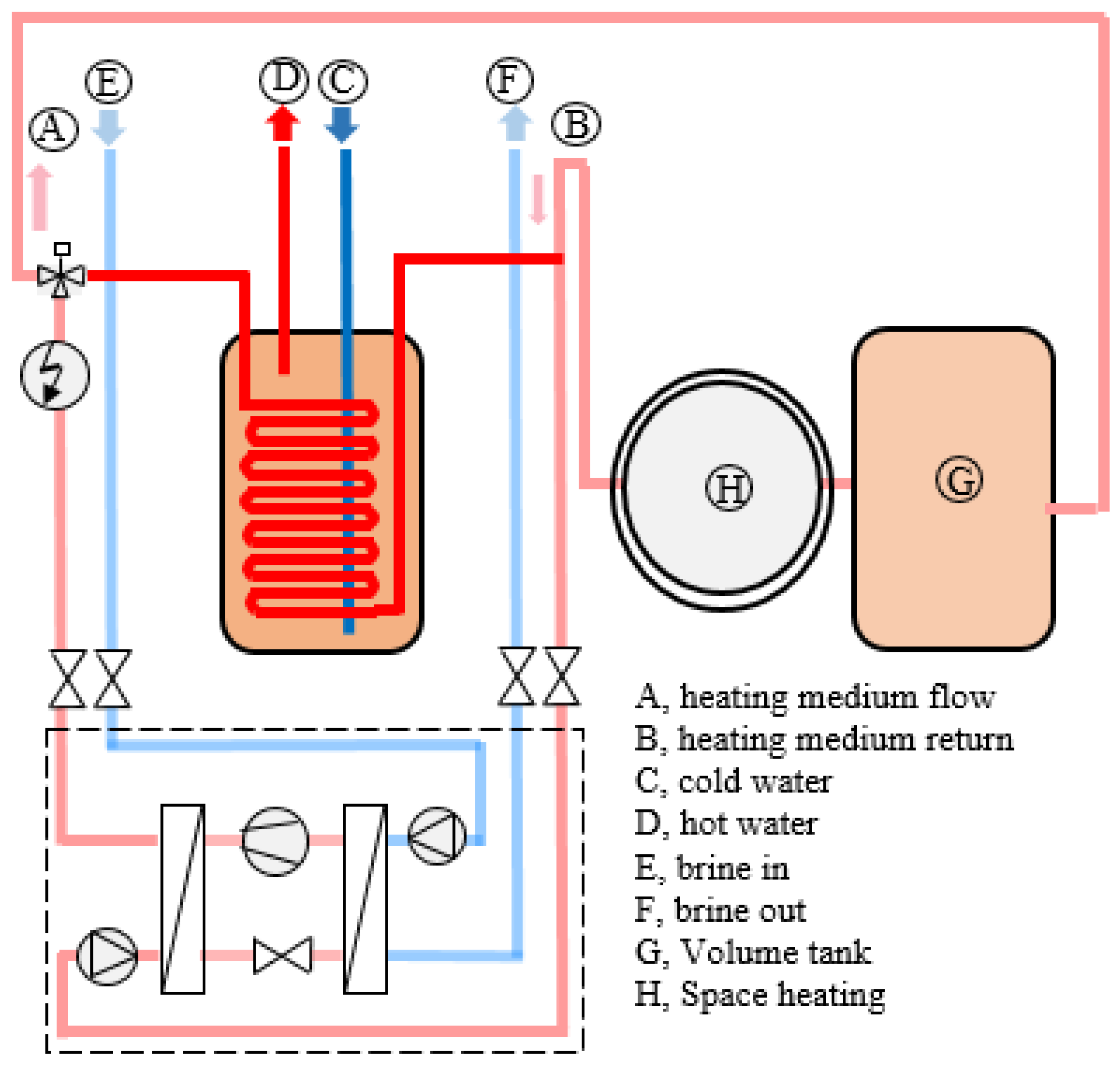
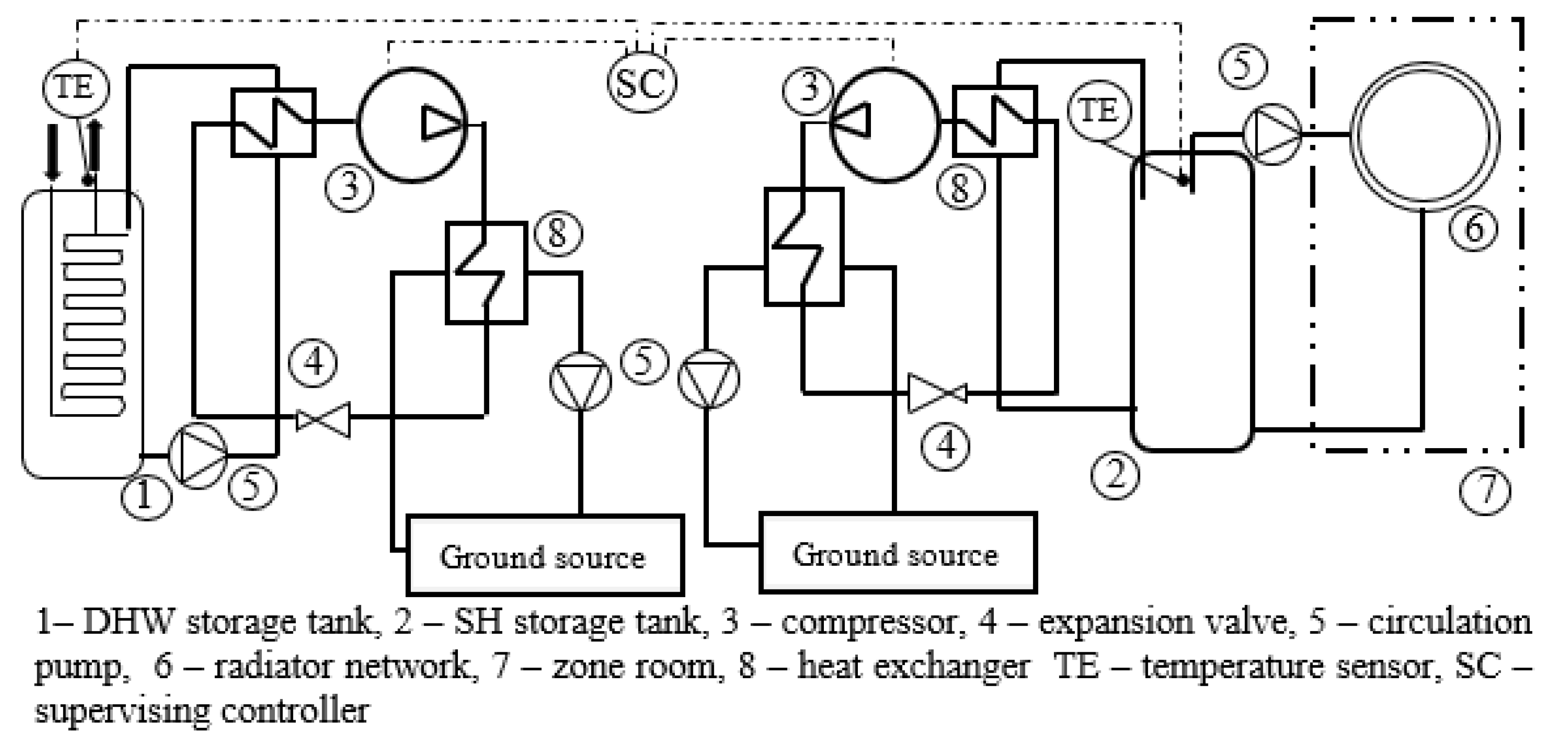
The working principle of common domestic GSHPs is shown in Figure 1. The system consists of a heat pump, heat source, heat sink, electrical module, circulation pumps, and a control system. GSHP is connected to the brine and heating medium circuits, which takes up the heat at a certain temperature and delivers the heat at a higher temperature. The performance of GSHP depends on heating curve set points, the heating system in a room, control strategy, and so on. Low-temperature radiator heating system can be used in low energy buildings and the heating curve might be higher than 5.0 °C compared to the floor heating system [25].
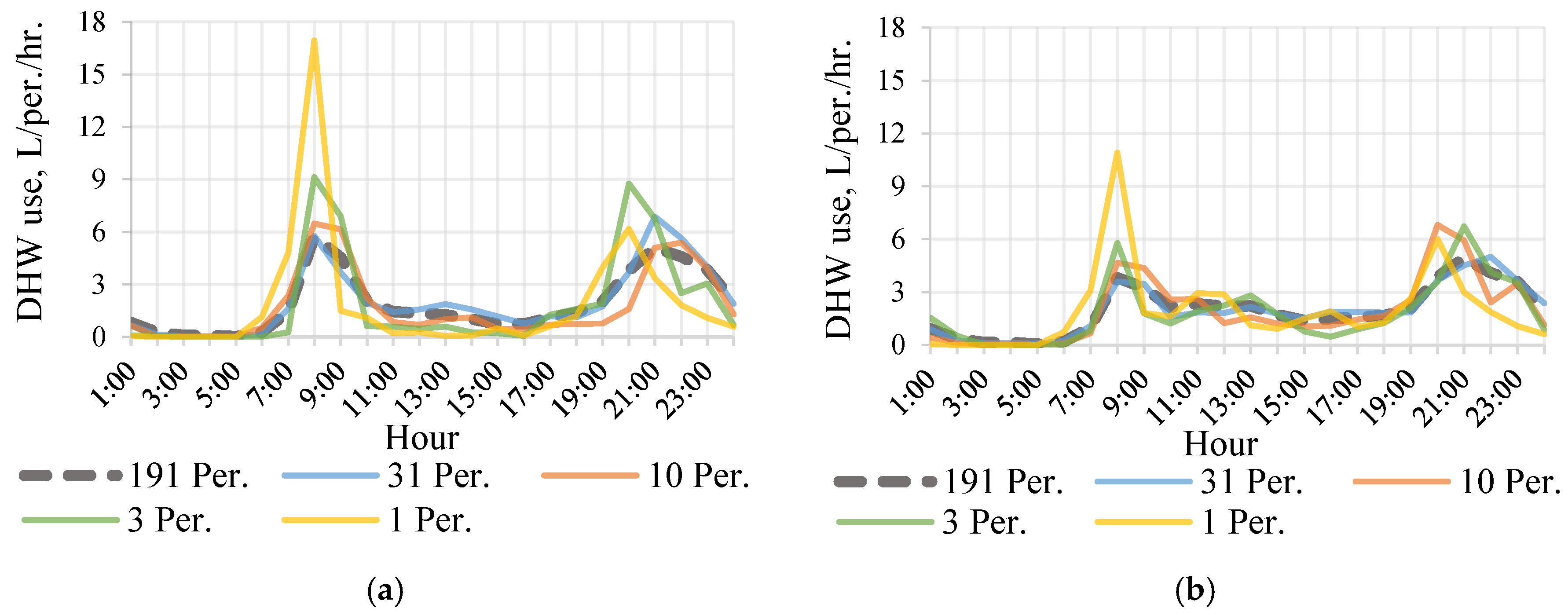
The objective of this study was to develop the alternate control model, allowing to determine the theoretical heating power need of a monovalent HP system at a designed outdoor temperature as a function of space and DHW heating needs. The hourly DHW usage profiles with two visible peaks, typical for single-family houses (Figure 2), were used for the power sizing of a GSHP. Besides, occupancy variations from three to six people in single-family houses, effects of internal heat gains were also considered in order to develop the sizing power equations for GSHP. Based on the determined heating power, a heat pump can be selected so that it covers 100% of the power or less of the power, that question was let out of the scope of this paper. The outlines of this study are the following:
- an alternate operational control system for GSHP was implemented in the IDA indoor climate and energy (IDA-ICE) plant model by developing a new control module, which was tested against measured data;
- maximum power was studied at different scenarios, i.e., occupant number, internal heat gains, building structural types, different design outdoor temperatures, DHW usage variations, variations of DHW usage peaks;
- equations that calculated the GSHP power at outdoor design temperature were developed and tested;
- the accuracy of equations was tested to calculate the GSHP’s power for old buildings (followed the Finnish 1976 building regulations), building in different climate regions, variations of DHW usages, and so on. These could show the suitability of the control system as well as the total power estimation of GSHP for buildings in central European countries and buildings that may require major renovations.
The findings of this study were expressed as the power equations at design temperature, allowing to determine 100% of the total heating for space and DHW heating for a single-family house. These equations can be applied for any types of HP power sizing, which has an alternative operational principle and hydronic heating system.
2. Method
2.1. Space Heating Load
Heat losses from a building can be calculated from Equation (1). Heat transfer coefficients of building components (such as façade, roof, floor, glaze), ventilation rate, air change rate, thermal bridges, and infiltration rate were estimated according to the Finnish building code [27].
where, , heating power for space (), , sum of transmission heat losses through building envelope (external wall, ground, roof, windows, doors, thermal bridges, etc.) (), , heat losses caused by infiltration (), , heat losses caused by ventilation (), , infiltration rate (), , air leakage rate of building envelope (), , envelope area (m2), x, factor that based on the building height. The values for single, double, 3–4 storied, 5 or more were 35, 24, 20, and 15, respectively [27].
The same approach was used to estimate the heat load for a heated space in FprEN12831-1 [20].
where, , design heat losses of the heated space of i (), , sum of transmission heat losses through building envelope of i (external wall, ground, roof, windows, doors, thermal bridges, infiltration, etc.) (), , design heat losses caused by ventilation of i (), , additional heating up power for the heated space of i ().
We used dynamic simulation in order to determine the power need for space heating, which also accounted for the infiltration rate, as shown in Equation (2). According to the Finnish building code, the design outdoor temperature and indoor heating set points were −26 °C and 21 °C, respectively [23]. Besides, we considered the outdoor design temperature of −15 °C (for Strasbourg) could show the suitability of GSHP’s power sizing equations. In addition, no solar heat gain was used for computational analysis. Furthermore, occupancy rate, unit load for lighting and appliance, usages profiles for single-family houses were summarized from References [28,29].
2.2. DHW Heating Load
We used the daily average DHW use of 43 L/person/day for Finnish residential buildings [30]. This average DHW use per day was multiplied with monthly consumption factor [30], which further distributed according to the hourly factors during 24 h of each a day [5], as shown in Figure 2. As GSHP’s power was sized for a single-family house, the occupant number was varied from three to six. Thus, the obtained daily DHW use for a single-family house was calculated by using the following equation:
where, , total DHW use by a single-family house (), , number of occupant (dimensionless), , monthly DHW usage factor (dimensionless), , DHW use by each occupant ().
The was distributed in hourly basis according to the DHW hourly profile of three people [5]. Besides, the three people’s DHW Weekday profile was used, because of having higher peaks compared to the three people weekend profile and three people total profile (all days that include weekdays and weekends) [5].
In addition to the dynamic simulation, the sizing power for a DHW heating was done according to the FprEN 12831-3:2016 standard [21]. The sizing steps for a DHW system are well defined in Reference [21], including the storage losses and DHW loading factor, compared to the Finnish standard [23]. According to the EN standard, power needs curve for DHW (needs curve) and power supply from the system (supply curve) was used. The need curve was determined by measuring the volume flow rate based on the load profile. Besides, temperatures of hot and cold water were considered. In order to develop the supply curve, available heat source and corresponding data such as storage thermal losses, distribution losses, power, and, system efficiency were also considered.
where, , effective power of water heating system (), , nominal power of heat generator (), , mean water temperature in storage tank at time t (°C), , cold water temperature (°C), , supply temperature from heat generators at time t (°C), , heat losses from storage at time t (), , distribution heat losses ), water density (), water heat capacity (), , design flow rate (), temperature of water withdrawn (°C), , mean water temperature of the storage tank at the time reheating is switched on (°C), , time constant of storage tank during loading (min), , time (min), , water mass in the storage volume (kg), , heat capacity of water in the storage volume (), , thermal transmittance of the heat exchanger (), , effective surface of the heat exchanger (m2).
2.3. Simulation Model
The IDA indoor climate and energy (IDA-ICE, version 4.7.1) simulation tool was used for computational analysis. The model was developed in an IDA-ICE advanced level interface, where users could connect system components, connection editing, output data logging, and so on. The model was developed in the early stage building optimization (ESBO) plant model, which is available in the tools library. IDA-ICE are well-established energy simulation tools, and many studies have been validated the reliability, performance, and accuracy compared to the field data [4,31,32,33,34].
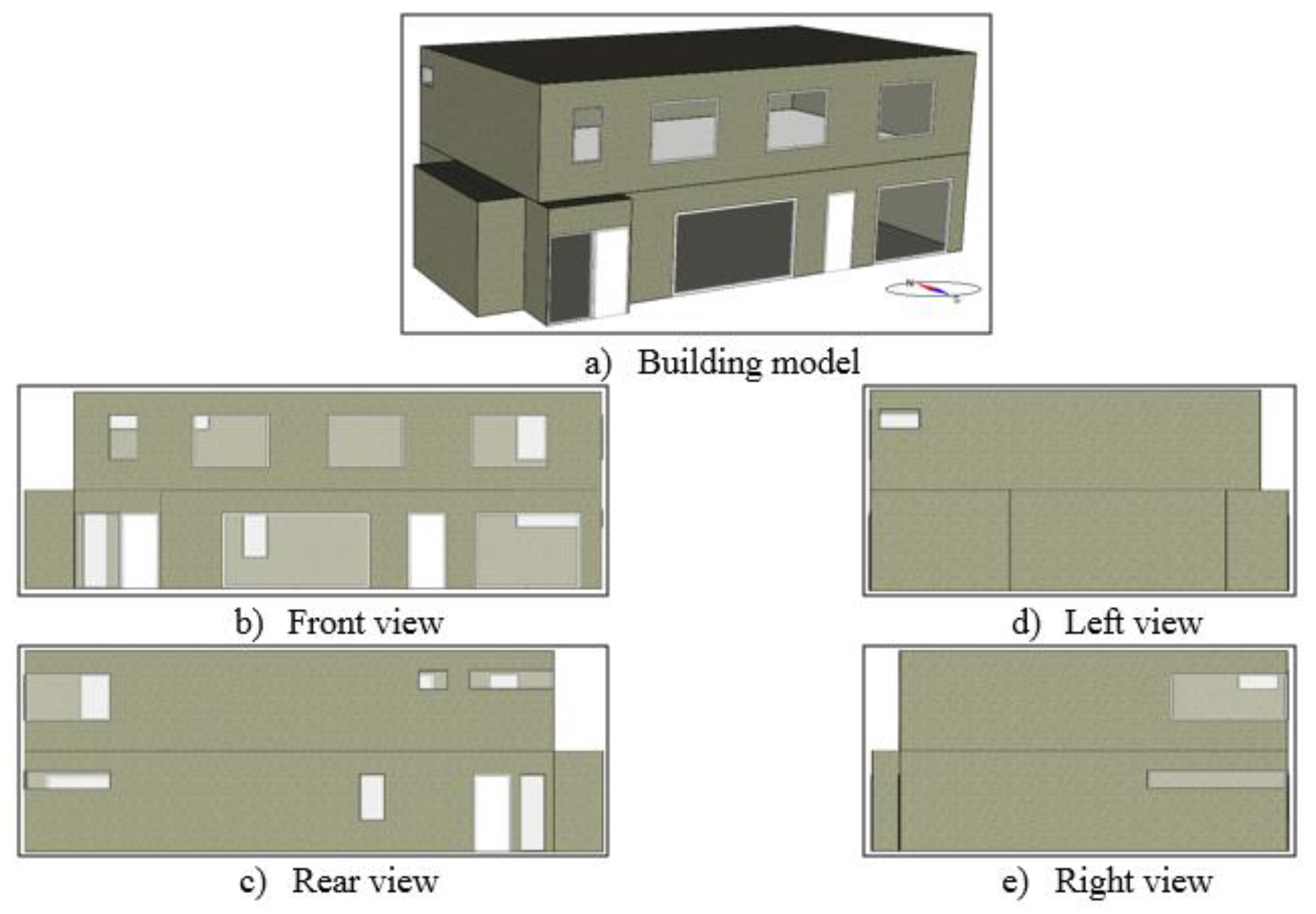
The reference single-family house with a heated net floor area of 171.1 m2 was used, as shown in Figure 3. It was assumed that the building model could use as a typical representative single-family house in Finland. Building input parameters were selected according to two building regulations, i.e., modern low energy (passive) building, old building regulation of 1976. The effects of heavyweight and lightweight construction concepts on indoor thermal condition were also discussed. The detailed building information is given in Table 1.
The external wall (from inside to outside) of a lightweight building consisted of gypsum board, air gap and EPS insulation. The heavyweight building used LECA block additionally. The external wall followed the old building regulation of 1976 and used the concrete wall instead of an LECA block. Roof structure (from inside to outside) consisted of gypsum board, air gap, and EPS insulation, wooden frame, and metal sheet. Similarly, the floor structure kept the same configuration (from inside to outside) for all cases, i.e., parquet, concrete, and EPS insulation. For the internal floor, a wooden floor slab was used in lightweight building cases whereas hollow concrete slab was used in heavyweight building cases. The internal floor of an old building followed the old building regulation of 1976 that used concrete floor. For the low energy building case, the model considered a balanced ventilation system with a heat recovery unit, Table 1. Thus, supply air was heated by recovered heat from the heat exchanger and heating coil. A low-temperature underfloor heating system (35/28 °C) with a PI controller was considered. The design power for underfloor heating system was 35 W/m2 at a maximum temperature drop of 7 °C. The pipe located at 0.035 m below from the floor surface top and heat transfer coefficient was 30 W/m2K.
For building model according to old building regulation of 1976, there was no air-handling unit. The model was equipped with a mechanical exhaust ventilation system only. The heating need was provided by a radiator system (55/45 °C) with a PI controller. A detailed radiator model (available in the IDA-ICE library) was considered, and total heat generation was calculated by using the following equation:
where, , heat flux from water (W), , coefficient of power law, which depends on the radiator height and width (), , difference between the mean surface temperature of radiator and the air temperature, , radiator length (m), K, radiator constant (dimensionless).
A stratified tank model with a capacity of 200 L was used. The tank model had five different layers, and it was highly insulated. This model also considered the storage heat losses and distribution heat losses.
3. Results and Discussion
3.1. GSHP and Control System Model
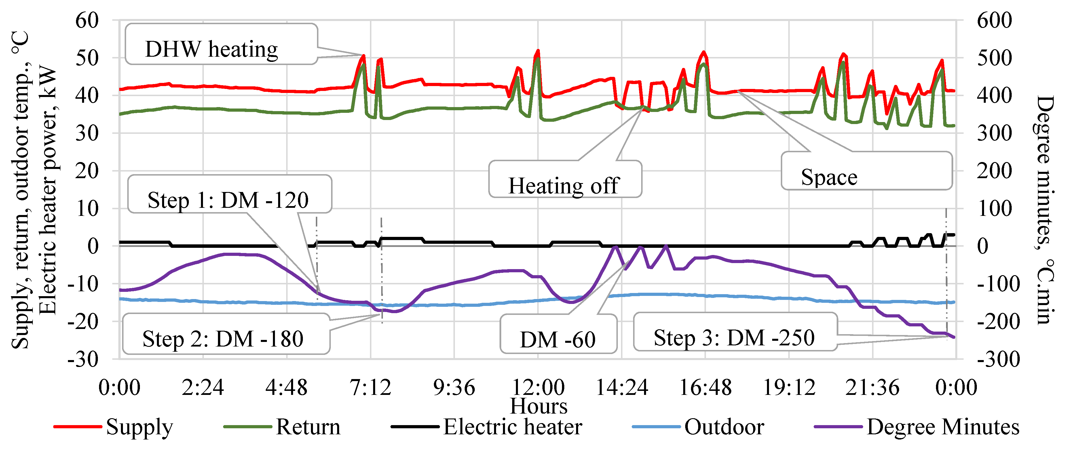
An existing GSHP alternate control strategy was followed, enabling to supply the heat either for space or DHW heating. In order to illustrate the operation principle of such type of HP, the measured data of GSHP during 24 h at one cold day are shown in Figure 4. This is an example, how the modeled control principle works in reality. Heat energy for space heating was supplied according to the heating curve. The corresponding deficits of heat were counted as degree minutes (DM) value. Similar to the degree day (DD) method, the DM value is a cumulative number of the difference between actual flow temperature (Ta) and setpoint temperature of flow (Ts) for given elapsed times in minutes. The default DM value with a couple of degree temperatures (as a dead band) were assigned in the control system setting. If the estimated DM value was fallen beyond the default value (in this case, −60 °C·min), the system would start immediately. In some extreme cases, if GSHP failed to supply sufficient heat, an electrical top-up heater switched on according to the default steps and fulfilled the need at the demand side. In this case, the top-up heater switched on in six steps based on the DM value. For instance, top up heater operated for step 1 (1 kW, −180 < DM < −120), step 2 (2 kW, −240 < DM < −180), step 3 (3 kW, −300 < DM < −240), step 4 (4 kW, −360 < DM < −300), step 5 (5 kW, −420 < DM < −360), and step 6 (6 kW, DM < −420).
The red line represents the supply water of temperatures for space and DHW heating. When GSHP ran in space heating mode, the supply water temperatures were in between 40 and 45 °C. Besides, if GSHP ran in a DHW heating mode, the supply water temperatures were higher than 45 °C (peak shown in Figure 4). In some periods the top-up electric heater switched on in a couple of steps in order to compensate the heat deficit. GSHP was in heating off mode if the DM value was higher than zero (heating off in Figure 4).
In this study, a monovalent ON/OFF brine to water GSHP (driven by electricity) was used to produce heat energy for space and DHW heating. The developed control system switched the heat generator either to DHW or to space heating (SH) mode, and it was forced to run the GSHP at the maximum load capacity during the operation period.
The GSHP control system accounted for the deficit of heat for space and DHW on a priority basis. The time interval was implemented in the plant model. The time interval means the maximum time to operate in one heating (space heating or DHW) mode if demand existed and after that time the HP pump was switched to another mode. The time interval was a user-defined value such as 15 min, 20 min, 30 min, etc.
The supply of heat was regulated according to the heating curve, and the set point temperature of delivered DHW. The control system calculated the deficits of heat as the DM value. Based on the DM value and delivered water temperature of DHW, the HP compressor was in ON/OFF mode. The differences were counted as DM value for each minute if and the cumulative number was obtained for a given elapsed minutes. The following equation was used to calculate the DM value:
where, degree minutes (°C·min), , heating curve setpoint temperature (°C), , flow temperature at actual condition (°C), , elapsed time (minutes).
The schematic diagram of the model is shown in Figure 5. For modeling of the periodic HP operation, two HPs were used in the model instead of one HP in reality. The model was designed in such a way that only one HP operated at a time or both HPs were switched off. The supervising control system was placed between the two HPs, which decided the active state of one HP among two HPs and ensured only one HP operation at the same time. One HP and one storage tank were operated for the space heating facility. Similarly, another HP and another storage tank were operated for DHW heating. The properties of both HPs’ and storage tanks were similar. The control system generated signals based on the heat deficits of space or DHW heating and then switched to SH mode, or DHW mode or OFF mode. In SH mode, only one HP for space heating was in operation, and another HP for DHW heating was switched off. Similarly, only one HP for DHW heating was in operation in DHW mode, and another HP for space heating was switched off. If there was no heat demand for space and DHW heating, both HPs were switched-off. Heating of each mode could be possible for a given time interval, which was a user-defined parameter. It could be possible to choose either 15 min, 20 min, 30 min interval and so on based on the demand side. This study considered the maximum time interval of 30 min after that HP switched to another mode. The control system follows the following steps, which is also illustrated in Figure 6.
- Step 1: DHW mode—started with DHW heating mode (DHW heating priority) for a maximum of 30 min. If continuous heating was required for DHW, the DHW mode would continue for a maximum period of 30 min. However, if no was heating required for DHW after some time interval, for instance, 15 min or 20 min of DHW heating period, the mode switched to SH mode (step 2) or OFF mode (step 3).
- Step 2: Space heating (SH) mode—continued for the next 30 min and afterwards retained back to step 1 if heat was required for DHW heating. If there were no heat demands for DHW heating but space heating, the SH mode would continue for the next 30 min period. If there were no heat demands for space and DHW, then it switched to OFF mode.
- Step 3: OFF mode—referred to as the state of GSHP where there was no heat demand for space and DHW heating that could allow the GSHP switched off.
It was a continuous process, which could able to provide heat for space and DHW heating. The best thing about this control system is that it is also suitable for extreme cases. For instance, at night time when the outdoor temperatures were very low, and the house had a less DHW consumption, the control system operated the GSHP at SH mode. It was able to continue at SH mode (because there were constant heat demands for SH and no heat demand for DHW), it would keep a stable indoor thermal condition. Similarly, at morning (for instance 7:00–8:00 h) when the peak demand of DHW was high, the control system operated the GSHP at both modes with a maximum interval of 30 min for each mode. It could keep the DHW supply temperature at an acceptable level.
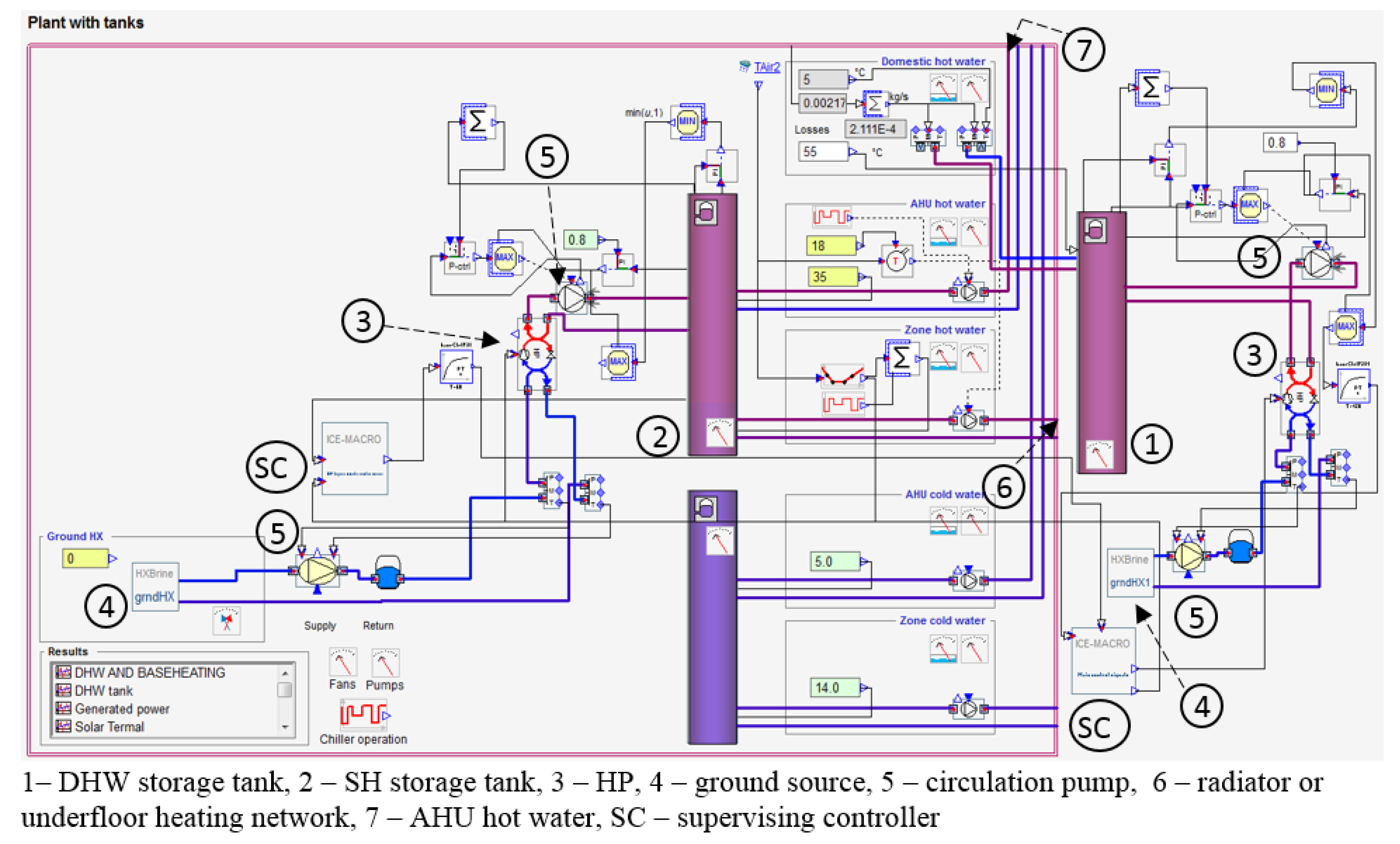
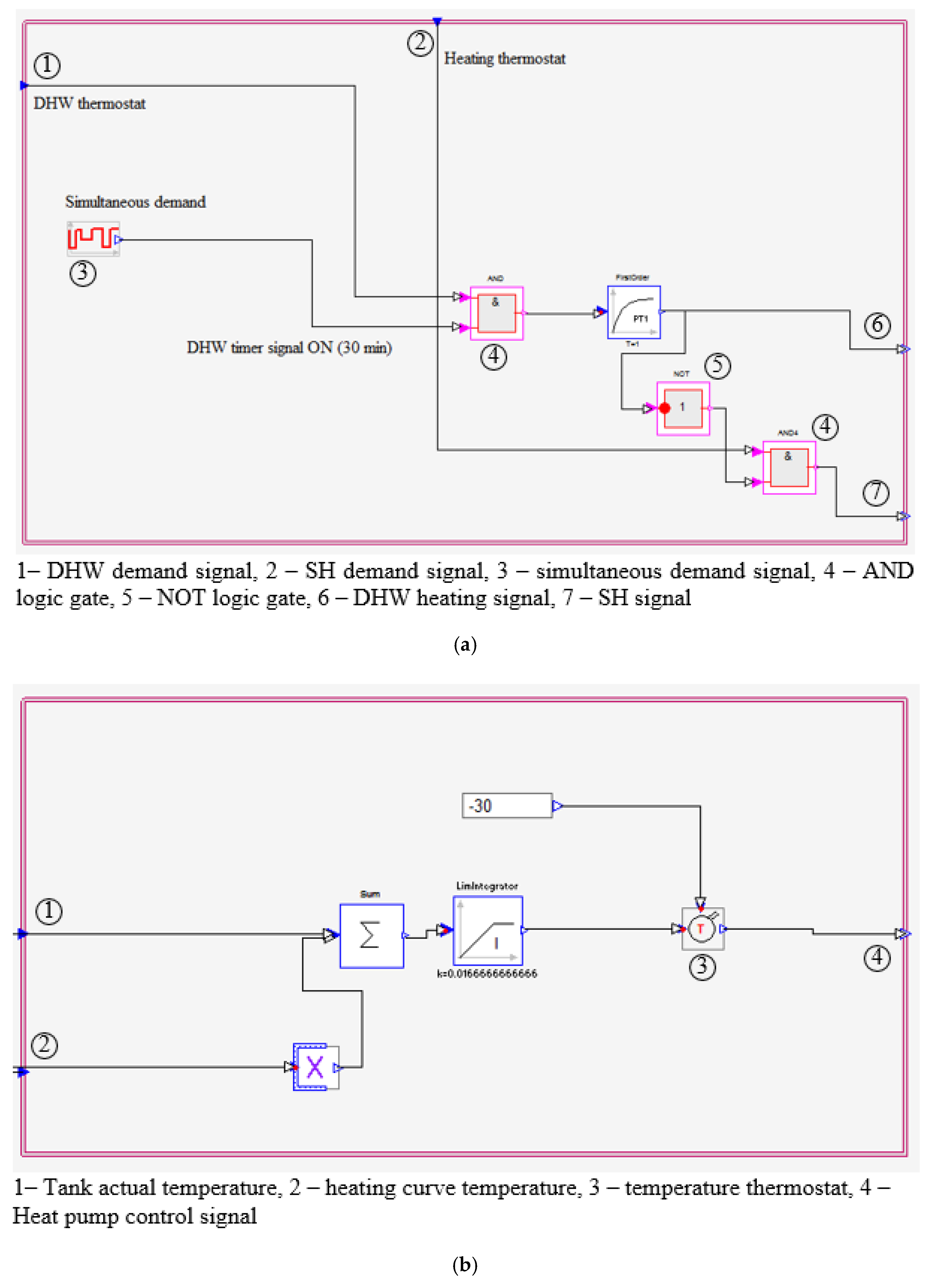
This schematic diagram of a model as shown in Figure 5 was implemented in IDA-ICE (Figure 7). The condenser side of GSHP was connected to the stratified tank to meet the heating demand side. No additional top-up heater was needed, and the heating curve was controlled according to the outdoor air temperature. GSHP also met the performance maps of manufacturer specific product. GSHP operated with maximum power whenever the temperature at demand side dropped below the heating setpoint temperature. The operation process was continued until it reached the desired setpoint temperature. Moreover, the model implemented in IDA-ICE, with two GSHPs and two storage tanks are shown in Figure 7. Besides, the detailed of heat pump’s control system is shown in Figure 8.
3.2. Operation Principle of the Control System
This section shows the operation of a control system according to the DM value. The control system recorded the delivered water temperature for space and DHW heating. If the delivered water temperature for space heating was less than the given set point temperature, the control system counted it as a heat demand signal for SH. Similarly, if DHW delivered temperature was less than 55 °C than the control system identified it as heat demand signal for DHW heating. Afterwards, the DM value was compared to the default setting value (user-defined DM value). The default setting value was considered as −60 °C·min (could be chosen between 0 to −120 °C·min). The GSHP compressor was in ON status and accelerated the heating production if the DM value was below than −60 °C·min. It also kept a similar status until the DM value reached zero. When DM was higher than zero, the GSHP compressor was switched off (OFF mode). During the on status, it worked according to the mentioned steps.
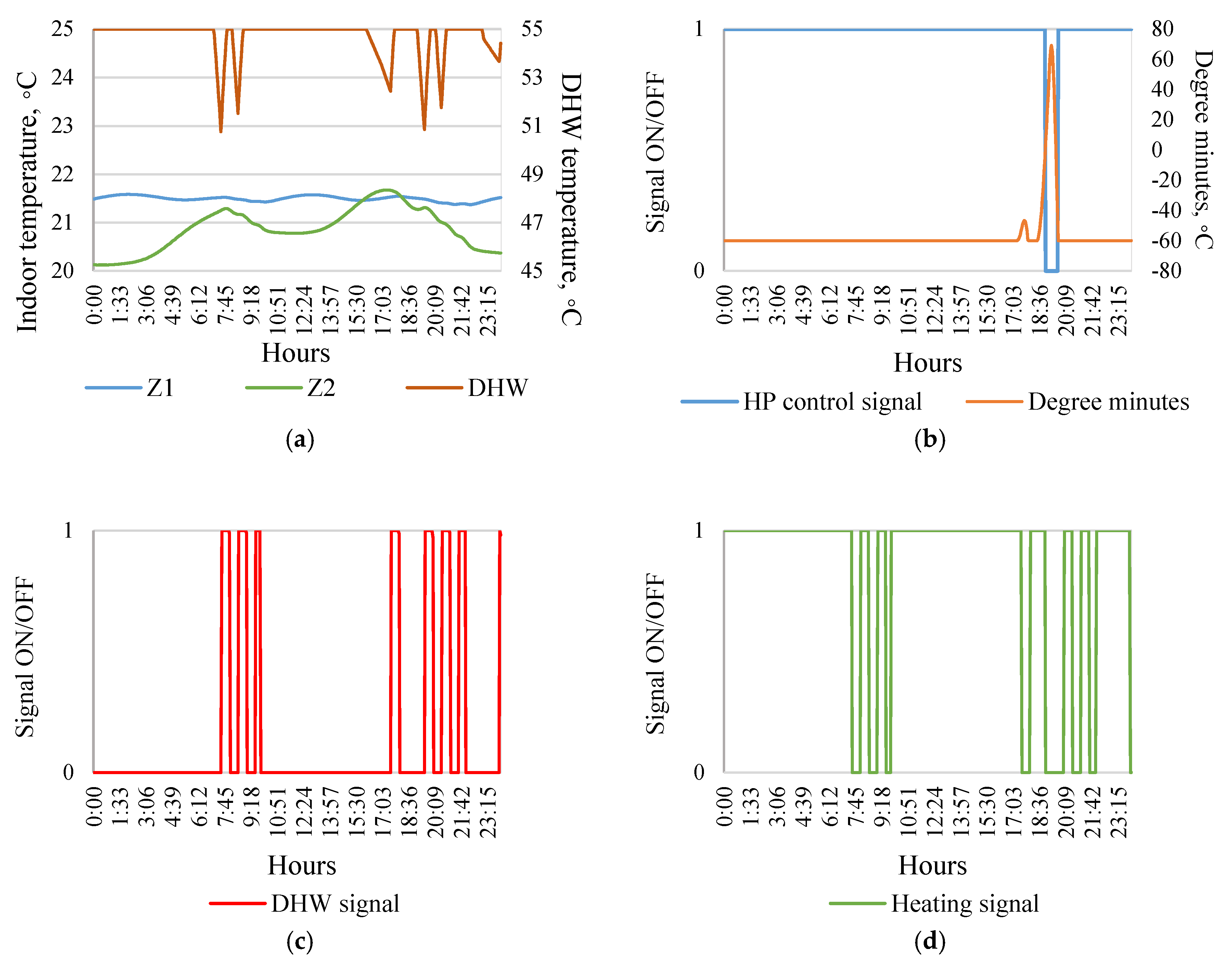
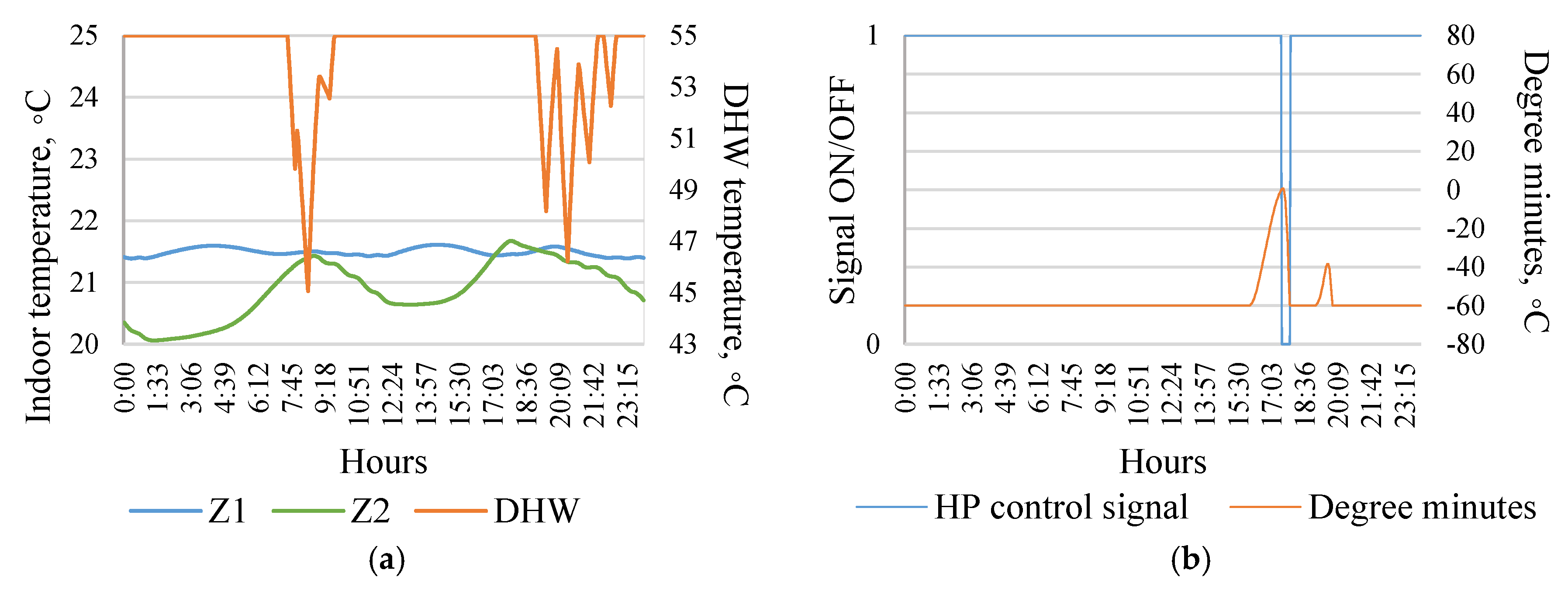
The dynamic simulation was performed during the heating season, i.e., 1st of December to 28th of February, 2018 and the results of indoor temperature, DHW outlet temperature, GSHP control signal, DHW signal, and heating signal for four people occupied a single-family house during 24 h are reported in Figure 9.
The control system determined the operational state of GSHP, i.e., ON, or OFF. The GSHP was in ON status for all hours in a day except 18:57 h (DM was 5.0 °C·min) to 19:39 h (DM was −42.8 °C·min), as shown in Figure 9b. During OFF mode, the DM was between 5.0 and −42.8 °C·min. However, the OFF mode happened at different times in different days because of the dynamic process. The indoor temperatures were higher than 21 °C for Zone 1 (Ground floor), and Zone 2 (First floor) and DHW outlet temperatures were not below than 51 °C (Figure 9a). Total heat deficits were estimated as the DM value, which was limited to −60 °C·min in this case. The GSHP started if DM was ≤−60 °C·min and it ran in DHW heating mode. GSHP ran in DHW heating mode for a maximum of 30 min, and alternatively, it switched to SH mode, if heating needs exist for SH.
The duration of DHW heating was short (9:33 to 9:48 h) due to the fulfilment of demand, as shown in Figure 9c. However, GSHP ran with SH mode for a minimum of 30 min duration, and it remained the same state if there would no heating demand for DHW, and continuous heating demand for space heating (Figure 9d). Besides, if the GSHP ran with SH mode and there was a continuous withdrawal of DHW from the tank, i.e., 7:06 to 7:27 h (Figure 9a); apparently the DHW outlet temperature was below the setpoint temperature. In this case, the DHW mode would not start immediately. It would start only after SH mode (minimum duration of SH mode was 30 min).
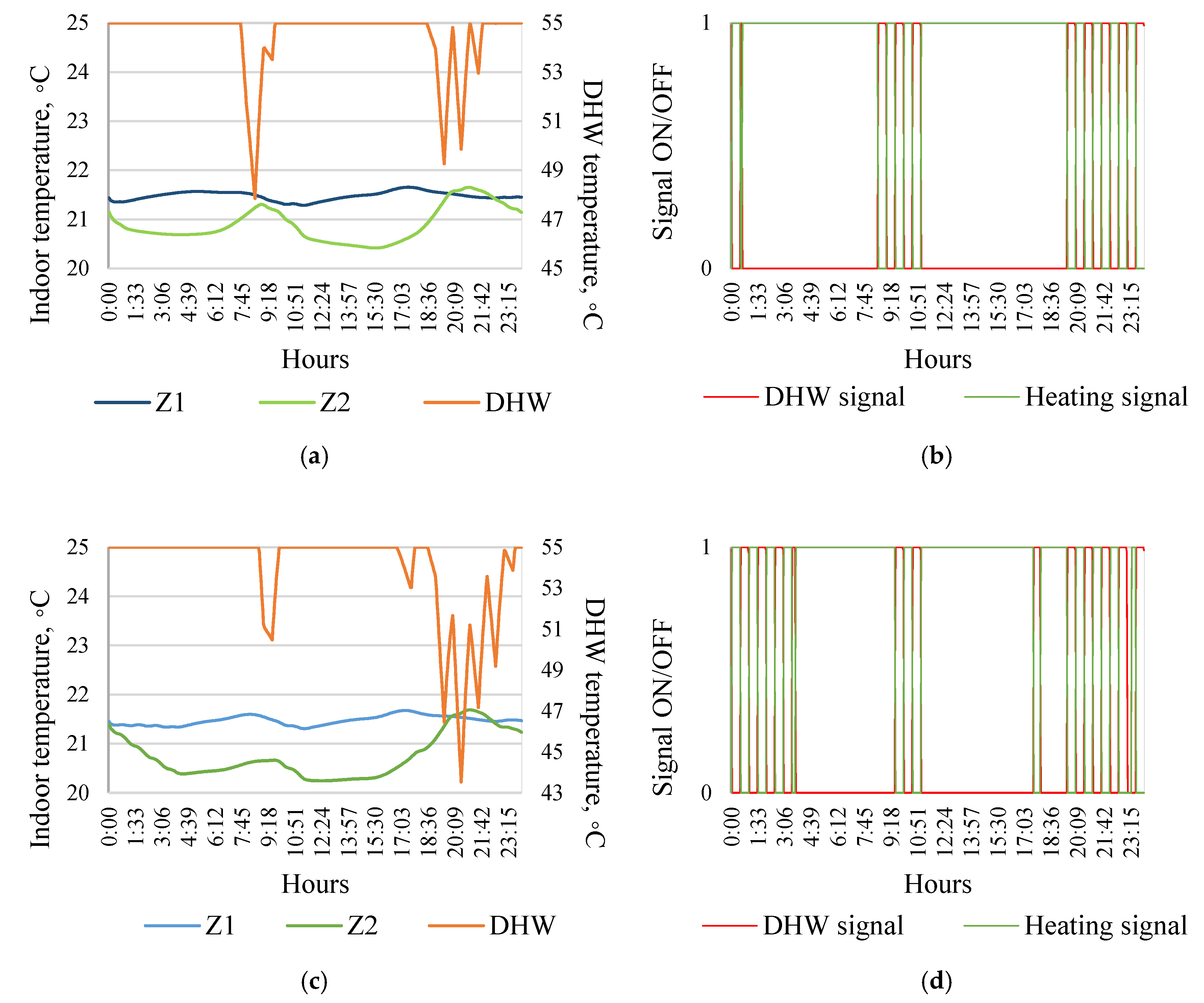
Energy use for DHW varied due to the different DHW usages volume, which mainly depended on the occupants’ number and hourly DHW profile. Heat demand for DHW heating had significant effects on system sizing compared to the constant space heating need. Indoor thermal condition, DHW outlet temperature, and GSHP operational signal for six people occupied single-family house are reported in Figure 10. The indoor temperatures were in the acceptable limit of Category II, according to EN 15251 [24]. During peak hours of DHW use, the outlet temperatures fell nearly 45 °C, which might be considered as the worst cases. These scenarios only happened if six people used the DHW at the same time in a single-family house.
3.3. GSHP Power Comparison
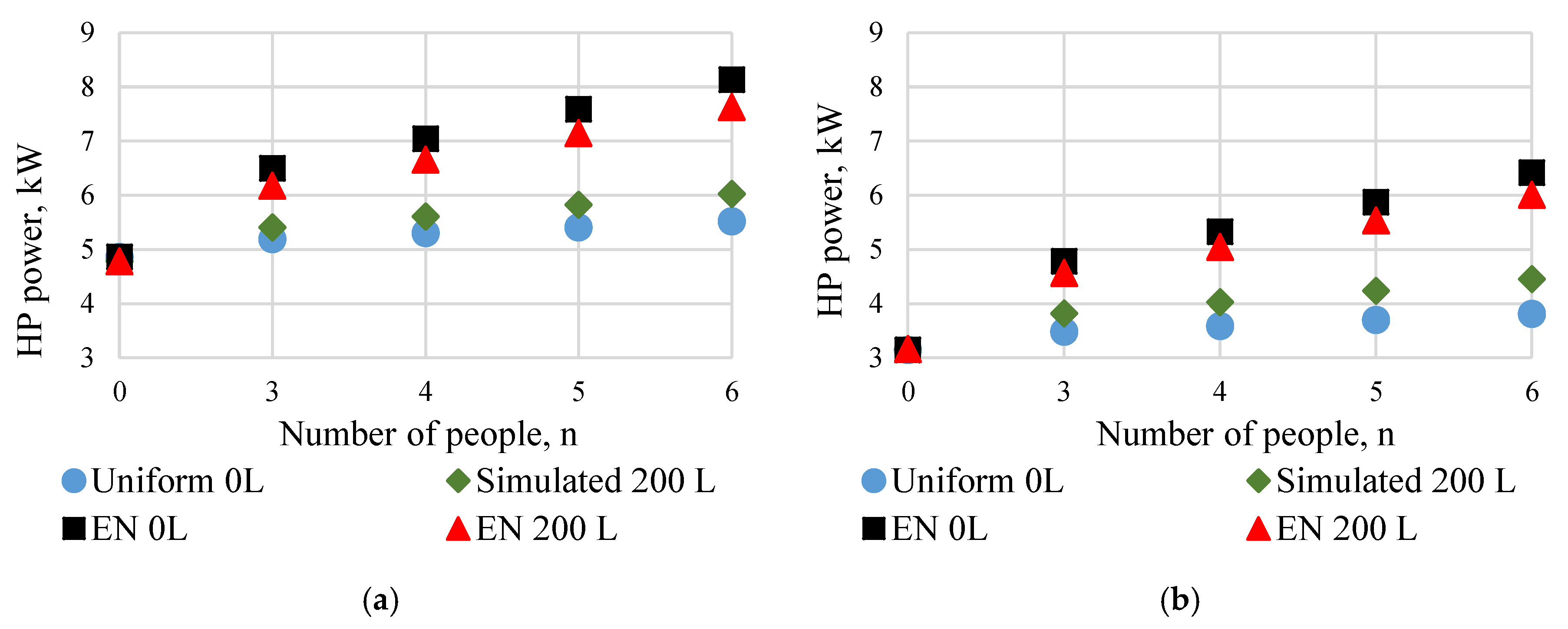
The total GSHP powers for a single-family house with different occupant groups were obtained by hand calculation and simulation approach, as shown in Figure 11. The hand calculation approach considered the steady state condition of DHW use with a uniform DHW profile and a three people DHW profile, following the Finnish building code [27]. Besides, the effects of storage tank were not accounted for. Daily DHW use was distributed equally into 24 h of a day and power of DHW heating was calculated for any hour (uniform 0 L). In the three people DHW profiles, the daily average DHW use was distributed according to the hourly usages factor, Figure 2. The maximum DHW usage volume was found at 8:00, which was used to calculate the maximum power required for DHW heating (EN 0 L). According to the Finnish building code [23], the heating power is the sum of simultaneous space heating, supply air heating, and DHW powers. Uniform 0 L case might not offer a realistic solution for single-family houses due to neglecting the hourly DHW consumption peaks. In addition, DHW and space heating powers were summed according to EN 0 L case, which led to overestimated GSHP power.
In the simulation approach, developed in this study, storage tank effects and DHW profile were considered. This Simulated 200 L case was compared with EN 200 L calculated according to the standard. In these both cases, a storage tank of 200 L was added. The Simulated 200 L case resulted in a 14%–44% power reduction compared to EN 0 L and EN 200 L cases, and the powers were 4%–14% higher compared to the non-realistic uniform 0 L case.
The hourly profile of DHW was not suitable for the‘EN 0 L’ case because peaks of DHW usage require a storage tank, which can compensate for the required thermal mass at the minute level. For ‘uniform 0 L’, DHW usages were distributed evenly, and no peaks occurred. These two cases demonstrated the manual calculation method in order to show how Finnish and EN regulations estimated the power at static condition. For all realistic cases, a ‘simulated 200 L’ water tank was used as shown in Figure 5.
3.4. Effect of Internal Heat Gains
The Finnish building code does not take into account the internal heat gains in order to estimate the design heat load [23]. However, EN standards account for the internal heat gain as optional heat load to estimate the design heat load [21]. DHW use and internal heat gains tend to appear simultaneously in a single-family house. Effect of internal heat gains was studied because it has a significant impact on system sizing, especially in low energy buildings. Moreover, solar heat gains were not accounted for system sizing due to the absence of solar heat during the night. The GSHP’s control system also performed while accounting internal heat gains. The indoor temperature, DHW outlet temperature, DHW signal, and space heating signal for four and six people’s occupied single-family house while considering internal heat gains are reported in Figure 12. Indoor temperatures for both zones (ground and first floor) were found in the acceptable limit (Category II of EN15251 standard) during the simulated period. The DHW outlet temperatures fell below the setpoint temperature at peak consumption hours, which was recovered when the GSHP ran with DHW heating mode (Figure 12a,c). Besides, GSHP ran with full power either for DHW heating mode or for SH mode (Figure 12b,d). The reduced HP sizing power with considering internal heat gains was calculated from Equation (12), Section 3.8.
3.5. Operational Performance of Control System at Different Scenarios
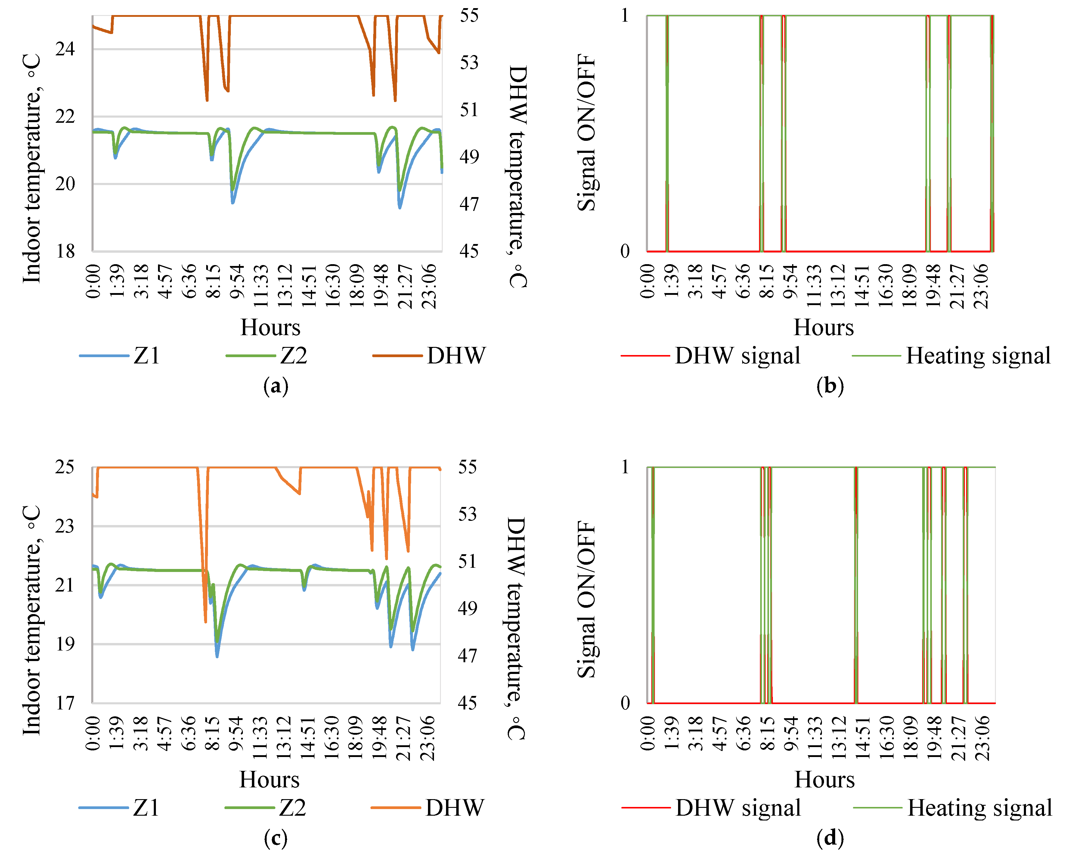
This section shows the suitability of this control system while sizing the heating power for old buildings (building parameters followed the old building regulation of 1976) or renovated buildings. The space heating need was higher compared to the low energy buildings and internal heat gains from occupant, lighting, and appliance did not seem so significant as low energy buildings. Heat losses from old buildings were quite fast so that the long duration heating mode could fail to serve the demand side. Duration of heating mode changed from 30 min to 15 min in order to keep the room temperature in an acceptable limit. According to the EN 15251 standard, the acceptable limit of indoor temperature must not be less than 18 °C (Category III) for old buildings [24]. GSHP operated with SH mode due to continuous space heating demand signals during the GSHP operation period. High GSHP power reduced the DHW heating mode duration, which allowed switching back to SH mode. Indoor temperature, DHW outlet temperature, DHW signal, and heating signal for houses occupied by four and six people are shown in Figure 13.
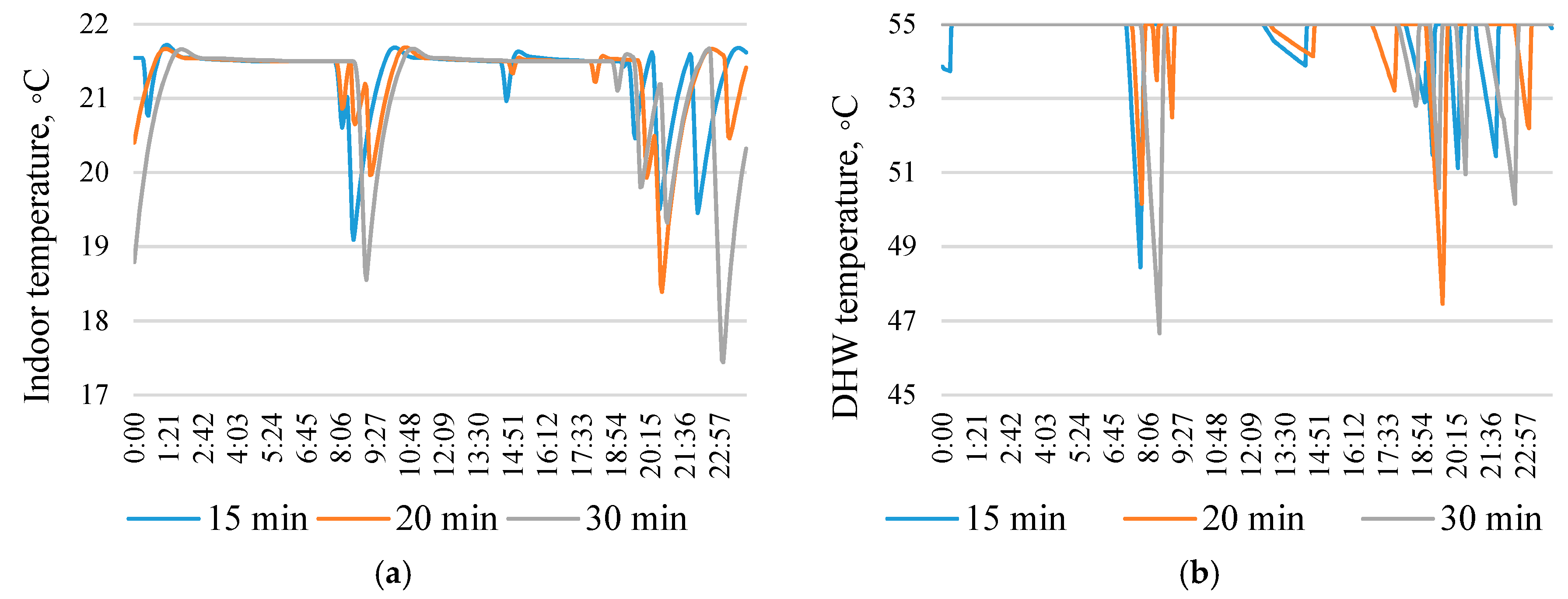
The effects of heating the mode duration on indoor temperature and DHW outlet temperature are reported in Figure 14. Effects were observed for those buildings, which required higher space and DHW heating. However, fewer effects were found in low energy buildings and building that occupied with a small group of occupants.
3.6. Simulation with Design Outdoor Temperature of −15 °C
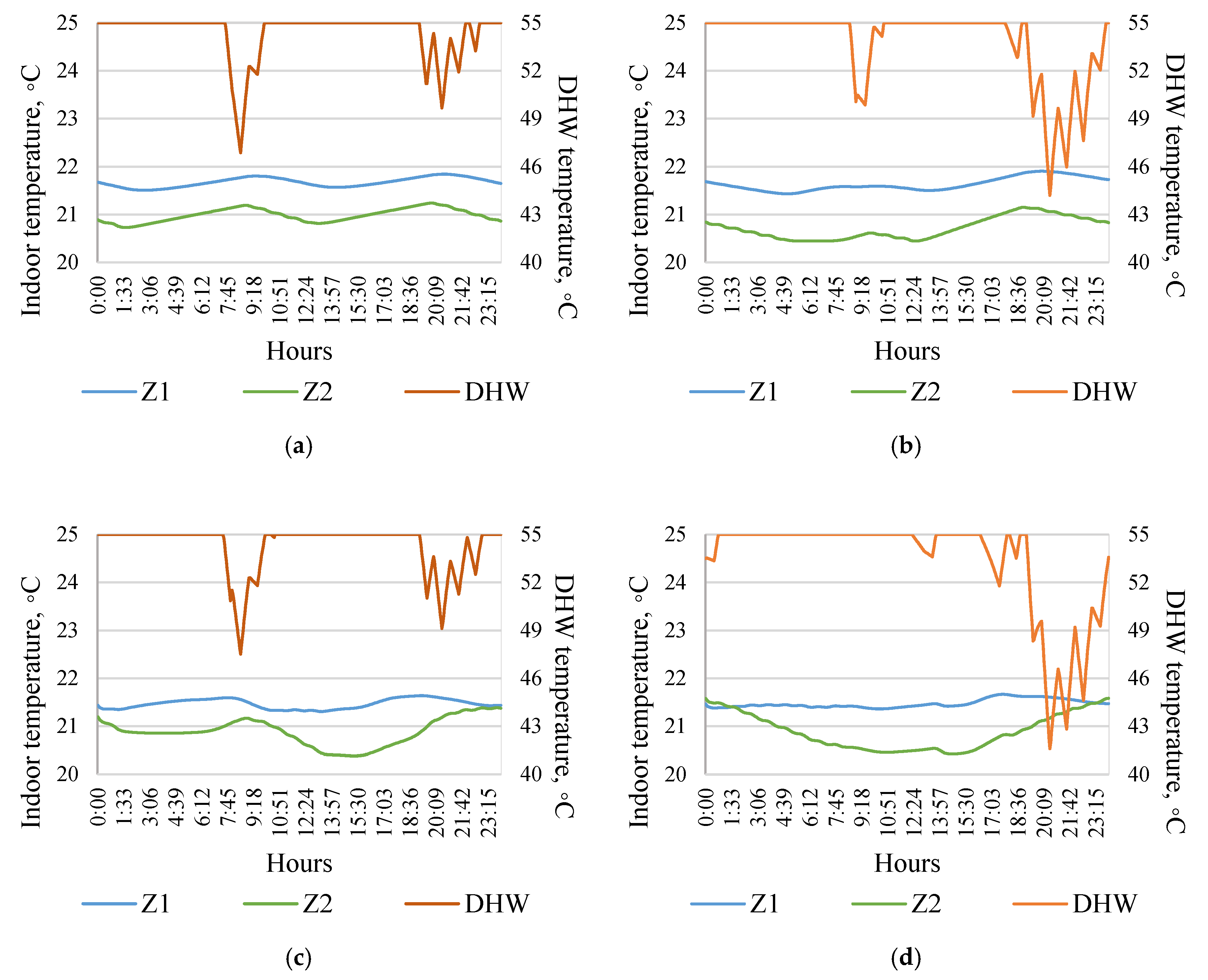
Simulations were repeated for another design temperature of −15 °C in order to validate the GSHP power equations in Section 3.8. In order to keep the same comparison platform, 30 min heating mode duration and internal gains also considered. Indoor temperature and DHW outlet temperature for four and six people’s occupied single-family house are shown in Figure 15. DHW outlet temperatures seemed critical compared to the indoor temperature. The GSHP power was low at a design temperature of −15 °C compared to the extreme Finnish case, i.e., −26 °C (Section 3.8). This low GSHP power resulted in the lower DHW outlet temperatures. This problem could overlook by picking the short heating mode duration, i.e., 20 min instead of 30 min.
3.7. Thermal Mass and Heating System Effects
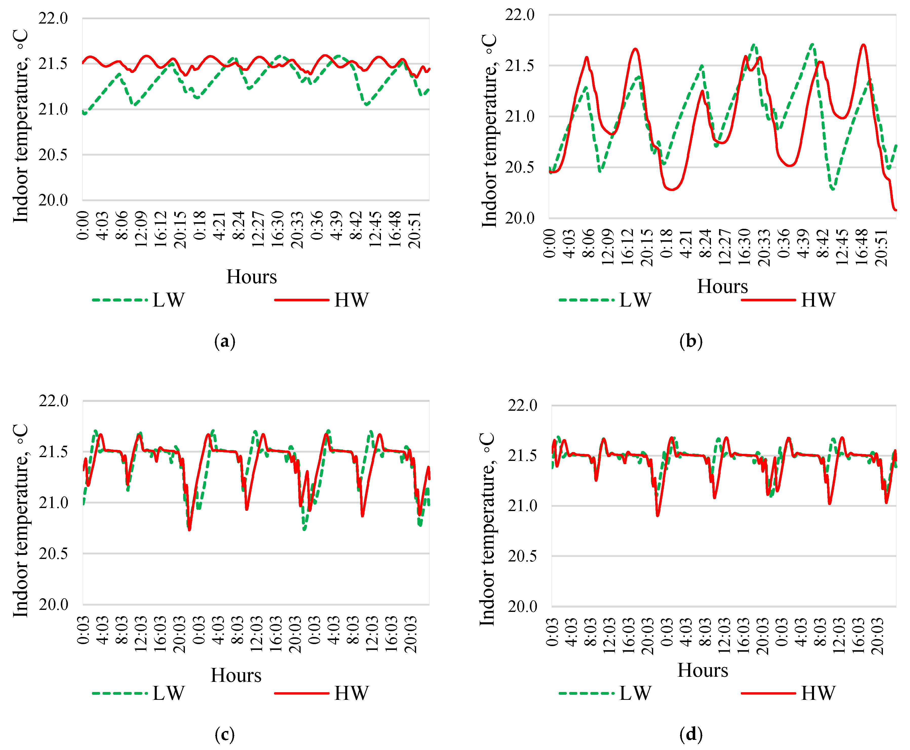
The effects of thermal mass and different space heating systems on indoor air temperature were evaluated in modern low energy passive building. Simulation with the LW, HW, radiator, and underfloor heating allowed us to analyze the effect of thermal mass and indoor heating solutions. The effects of the thermal mass were not significant, and are reported in Figure 16. No significant difference in indoor temperature was found due to the structural differences, i.e., HW, LW (Figure 16a,b). In addition, radiator heating was simulated, and results showed no significant difference in indoor air temperature between underfloor heating and radiant floor heating (Figure 16). The difference likely could not be seen because the HP periodic operation interval was so small (30 min) so that only the first centimeters of the structure were active. Active thermal masses were very limited because of the 30 min interval of heating.
3.8. Equations for GSHP Power
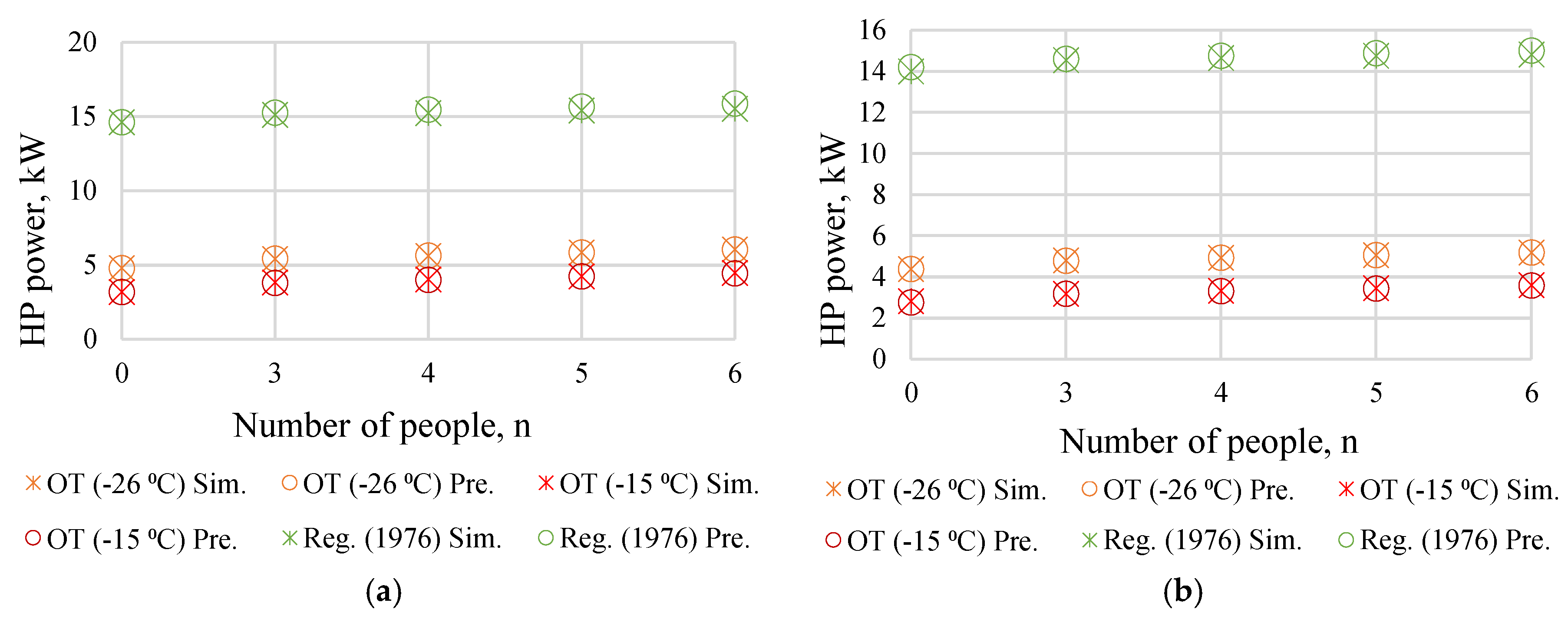
The simulated results were used to set up the heating power equations. The simulated GSHP powers were obtained for different occupant groups, alongside with internal heat gains, building that were built according to new and old building regulations of 1976, and at different design temperatures. Simulated power refers to the dynamic simulation results. The empirical equations for GSHP power estimation were developed based on simulated results, which were tested for different scenarios. Total design power of GSHP can be estimated with Equation (11) for the case of without internal heat gains. However, internal heat gains cut-off a good percentage of space heating demand, which may be taken into account for the system’s power sizing in low energy buildings, Equation (12). The simulated and predicted GSHP powers are shown in Figure 17.
where, , GSHP power (kW), , total heat losses from building (kW), C, constant (C = 0.21 for case of 3 people DHW usage profile, where daily consumption rate of 47 ), n, number of people in house (n = 3, 4, 5, 6), A, floor area (m2), , usages rate of lighting (dimensionless), , unit load for lighting (), , usages rate of appliances (dimensionless), , unit load for appliances (), , usages rate of occupancy (dimensionless), , body heat loss ().
The predicted GSHP powers, obtained from empirical Equations (11) and (12), showed a good agreement with the simulated results. The predicted results varied 0%–2.2% compared to the simulated values for both cases (Figure 17a,b). The required GSHP power, with internal heat gains, reduced the total heating powers by 3%–19%. Higher effect of internal heat gains was found in new modern buildings compared to old buildings. Besides, the effects were more visible for buildings in Strasbourg (design temperature of −15 °C) compared to the Finnish buildings (design temperature of −26 °C). In the case of a house occupied by three people, the internal heat gain effect (the reduction of 0.63 kW) exactly compensated for the effect of the DHW (an increase of 0.62 kW). Furthermore, DHW heating power accounted for 21%–41% of the total heating power in the modern building with a design temperature of −15 °C and 13%–26% with a design temperature of −26 °C. The contributions of DHW heating in the old building were only in between 3% and 9%.
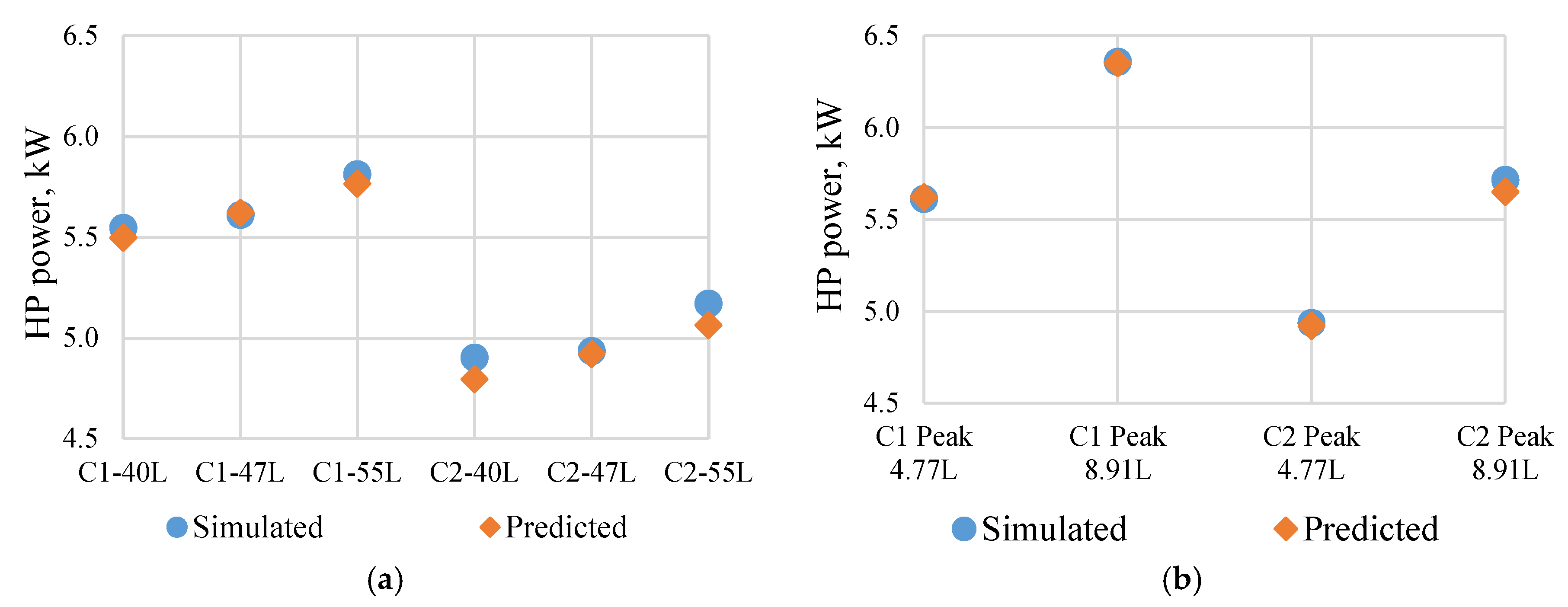
The performance of equations was tested for cases of different daily, and peak DHW, uses. The GSHP power for different daily DHW use and hourly peaks can be calculated by using Equations (13) and (14), respectively.
where, Q1, DHW usage for given reference case (), C1, constant for given reference case (dimensionless), Q2, new DHW’s usage rate (), C2, constant (dimensionless) (constant obtained for case of new DHW’s usage rate or new DHW’s peak demand), P1, peak demand for given reference case (), P2, new DHW’s peak demand ().
With this GSHP control system, C1 was equivalent to 0.21 for a case of three people DHW profiles, where reference case had a daily usage rate of 47 L/person/day [30] and a peak demand of 4.77 L/person/h [5]. The obtained value of C2 was used in Equations (11) and (12) in order to estimate the GSHP power. This study obtained the GSHP powers for daily usage rates of 40, 47, 55 L/person and for daily peaks of 4.77, 8.91 L/person/hour, as shown in Figure 18.
The predicted GSHP powers had shown a good agreement with the simulated results. For the case of different daily consumptions, the variation was found to be 0%–2% compared to the simulated results. Besides, the developed equations predicted the GSHP powers more precise for the case of different usage peaks. The impact of internal heat gains is well visible in Figure 18. The cutoff powers of GSHP were estimated at 11%–14% for cases with considering the internal heat gains.
4. Conclusions
This study developed an alternate operational control system for GSHP, which was applied to determine the total space and DHW heating power equations at design temperature for single-family houses. Data obtained from previous studies such as a daily average of DHW use, hourly DHW profile, occupancy profile, appliances profiles, lighting profiles were used in the whole building simulation model. The performance of the developed control model was tested against measured data. Reference building properties, different DHW usage rates and design temperatures of −26 °C and −15 °C were used in order to size the total design power of GSHP for modern and old single-family houses. The following conclusions can be drawn:
- The alternate operational principle of GSHP was implemented in IDA-ICE whole building simulation model. The GSHP’s control system was modeled with DHW priority switching from SH to DHW heating mode based on demand-side signals and a given duration of the heating period.
- The control of heat deficiency was modeled based on DM accounting. The default DM value (Section 3.1) and heating mode duration were user-defined, which enabled us to fit the GSHP operation for new and old buildings in different climates.
- Simulated GSHP system with a 200 L storage tank resulted in a 13%–26% power reduction compared to the calculation of the same system with EN standards, which required separate space heating and DHW power calculation.
- The periodic operation utilized the thermal mass of the building, and the sensitivity analyses with light and heavyweight buildings revealed the same effect because of the very short heating cycle of 30 min. With room a temperature setpoint of 21 °C, room temperatures only slightly decreased, so that indoor thermal comfort of Category II in a modern house and Category III in an old house were achieved. Besides, the DHW outlet temperature was in an acceptable limit.
- The contribution of DHW heating formed 2%1–41% of total heating power in a modern building with a design temperature of −15 °C and 13%–26% with a design temperature of −26 °C.
- Internal heat gains reduced the GSHP powers by 3%–19% when taken into account in the simulation. In the case of a house occupied by three people, the internal heat gain effect (the reduction of 0.63 kW) exactly compensated for the effect of the DHW (an increase of 0.62 kW). It brings a question, should the effect of internal heat gains be taken into account for heat pump sizing in low energy buildings?
- The total heating power equation was obtained in the form of the space heating power at a design temperature plus 0.21 kW of the DHW heating power per person. The equation was tested in modern and old single-family houses with design temperatures of −15 °C and −26 °C where the deviations remained between 0%–2.2%. It was demonstrated that the equations could be easily modified for different DHW daily usages or peak usages. For that purpose, other equations were provided.
Author Contributions
K.A. wrote the paper and conceived, designed, and performed the simulations. J.F. conceived and developed the initial control model. J.K. was the principal investigator responsible for the study design.
Funding
This research received no external funding.
Acknowledgments
This research was supported by the K.V. Lindholms Stiftelse foundation and by Estonian Centre of Excellence in Zero Energy and Resource Efficient Smart Buildings and Districts, ZEBE, grant 2014-2020.4.01.15-0016 funded by the European Regional Development Fund.
Conflicts of Interest
The authors declare no conflict of interest.
Abbreviation
| A | Floor area: m2 |
| Unit load for appliances, | |
| Envelope area, m2 | |
| Effective surface area of the heat exchanger, m2 | |
| Usages rate of appliances, dimensionless | |
| C | Constant, dimensionless |
| Water heat capacity, | |
| C1 | Constant for given reference case, dimensionless |
| C2 | Constant, dimensionless |
| degree minutes, °C·min | |
| Difference between the mean surface temperature of a radiator and the room’s air temperature, °C | |
| Monthly DHW consumption factor, dimensionless | |
| K | Radiator constant, dimensionless |
| Radiator length, m | |
| Unit load for lighting, | |
| Usages rate of lighting, dimensionless | |
| Water mass in the storage volume, kg | |
| Number of occupants, dimensionless | |
| Power law coefficient, which depends on the radiator type and width, | |
| Usages rate of occupancy, dimensionless | |
| Body heat losses, | |
| GSHP’s power, kW | |
| Heat flux from the water, W | |
| P1 | Peak demand for a given reference case, |
| P2 | New DHW peak demand, |
| Q1 | DHW consumption for a given reference case, |
| Q2 | New DHW consumption rate, |
| Infiltration rate, | |
| Air leakage rate of building’s envelope, | |
| Time, minutes | |
| Elapsed time, minutes | |
| Actual flow temperature, °C | |
| Cold water temperature, °C | |
| Supply temperature from a heat generator at time t, °C | |
| Flow temperature’s set point, °C | |
| Mean water temperature in a storage tank at time t, °C | |
| Mean water temperature of the storage tank at the time the reheating is switched on, °C | |
| Water withdrawn temperature, °C | |
| U | Thermal transmittance, |
| Thermal transmittance of the heat exchanger, | |
| Design flow rate, | |
| DHW consumption by each occupant, | |
| Total DHW consumption by a single-family house, | |
| x | Factor that based on the building height, dimensionless |
| Total heat losses from the building, | |
| Effective power for water heating, | |
| Design heat losses of the heated space of i, | |
| Additional heating up power for the heated space of i, | |
| Heat losses caused by infiltration, | |
| Nominal power for a heat generator, | |
| Space heating power, | |
| Sum of transmission heat losses through building’s envelope, | |
| Sum of design transmission heat losses through building’s envelope of i, | |
| Heat losses caused by ventilation, | |
| Design heat losses caused by ventilation of i, | |
| Distribution heat losses, | |
| Heat losses from a storage tank at time t, | |
| Water density, | |
| Time constant of storage tank during the loading period, minute |
References
- Ahmed, K.; Pylsy, P.; Kurnitski, J. Domestic hot water profiles for energy calculation in Finnish residential buildings. In Proceedings of the Young Researcher International Conference on Energy Efficiency, Linz, Austria, 25–26 February 2015. [Google Scholar]
- Ahmed, K.; Pylsy, P.; Kurnitski, J. Hourly consumption profiles of domestic hot water for Finnish apartment buildings. In Proceedings of the CLIMA 2016 12th REHVA World Congress, Aalborg, Denmark, 22–25 May 2016. [Google Scholar]
- Ferrantelli, A.; Ahmed, K.; Pylsy, P.; Kurnitski, J. Analytical modelling and prediction formulas for domestic hot water consumption in residential Finnish apartments. Energy Build. 2017, 143, 53–60. [Google Scholar] [CrossRef]
- Niemela, T.; Manner, M.; Laitinen, A.; Sivula, T.M.; Jokisalo, J.; Kosonen, R. Computational and experimental performance analysis of a novel method for heating of domestic hot water with a ground source heat pump system. Energy Build. 2018, 161, 22–40. [Google Scholar] [CrossRef] [Green Version]
- Ahmed, K.; Pylsy, P.; Kurnitski, J. Hourly consumption profiles of domestic hot water for different occupant groups in dwellings. Sol. Energy 2016, 137, 516–530. [Google Scholar] [CrossRef]
- Rodriguez-Hidalgo, M.C.; Rodriguez-Aumente, P.A.; Lecuona, A.; Legrand, M.; Ventas, R. Domestic hot water consumption vs. solar thermal energy storage: The optimum size of the storage tank. Appl. Energy 2012, 97, 897–906. [Google Scholar] [CrossRef] [Green Version]
- Yrjölä, J.; Laaksonen, E. Domestic hot water production with ground source heat pump in apartment buildings. Energies 2015, 8, 8447–8466. [Google Scholar] [CrossRef]
- Hervas-Blasco, E.; Pitarch, M.; Navarro-Peris, E.; Corberan, J.M. Optimal sizing of a heat pump booster for sanitary hot water production to maximize benefit for the substitution of gas boilers. Energy 2017, 127, 558–570. [Google Scholar] [CrossRef]
- Stafford, A. An exploration of load-shifting potential in real in-situ heat-pump/gas-boiler hybrid systems. Build. Serv. Eng. Res. Technol. 2017, 38, 450–460. [Google Scholar] [CrossRef] [Green Version]
- Bagarella, G.; Lazzarin, R.; Noro, M. Sizing strategy of on–off and modulating heat pump systems based on annual energy analysis. Int. J. Refrigerat. 2016, 65, 183–193. [Google Scholar] [CrossRef]
- Hakamies, S.; Hirvonen, J.; Jokisalo, J.; Knuuti, A.; Kosonen, R.; Niemela, T.; Paiho, S.; Pulakka, S. Heat Pumps in Energy and Cost Efficient Nearly Zero Energy Buildings in Finland. Teknologian tutkimuskeskus VTT Oy, 2015. Available online: https://www.vtt.fi/inf/pdf/technology/2015/T235.pdf (accessed on 2 June 2019).
- Rawlings, R.H.D.; Sykulski, J.R. Ground source heat pumps: A technology review. Build. Serv. Eng. Res. Technol. 1999, 20, 119–129. [Google Scholar] [CrossRef]
- Rivoire, M.; Casasso, A.; Piga, B.; Sethi, R. Assessment of energetic, economic and environmental performance of ground-coupled heat pumps. Energies 2018, 11, 1941. [Google Scholar] [CrossRef]
- Li, H.; Xu, W.; Yu, Z.; Wu, J.; Sun, Z. Application analyze of a ground source heat pump system in a nearly zero energy building in China. Energy 2017, 125, 140–151. [Google Scholar] [CrossRef]
- El-Baz, W.; Tzscheutschler, P.; Wagner, U. Experimental study and modeling of ground source heat pumps with combi-storage in buildings. Energies 2018, 11, 1174. [Google Scholar] [CrossRef]
- Dong, B.; Lam, P.K. A real-time model predictive control for building heating and cooling systems based on the occupancy behavior pattern detection and local weather forecasting. Build. Simul. 2014, 7, 89–106. [Google Scholar] [CrossRef]
- Arabzadeh, V.; Alimohammadisagvand, B.; Jokisalo, J.; Siren, K. A novel cost-optimizing demand response control for a heat pump heated residential building. Build. Simul. 2018, 11, 533–547. [Google Scholar] [CrossRef]
- Bouheret, S.; Bernier, M. Modelling of a water-to-air variable capacity ground-source heat pump. Taylor Francis 2017, 11, 283–293. [Google Scholar] [CrossRef] [Green Version]
- Salque, T.; Marchio, D.; Riederer, P. Neural predictive control for single-speed ground source heat pumps connected to a floor heating system for typical French dwelling. Build. Serv. Eng. Res. Technol. 2014, 35, 182–197. [Google Scholar] [CrossRef]
- FprEN 12831-1. Energy Performance of Buildings—Method for Calculation of the Design Heat Load—Part 1: Space Heating Load, Module M3-3; EPB Center: Chattanooga, TN, USA, 2016. [Google Scholar]
- FprEN 12831-3. Energy Performance of Buildings—Method for Calculation of the Design Heat Load—Part 3: Domestic Hot Water Systems Heat Load and Characterisation of Needs, Module M8-2, M8-3; EPB Center: Chattanooga, TN, USA, 2016. [Google Scholar]
- FprEN 15316-4-2. Energy Performance of Buildings—Method for Calculation of System Energy Requirements and System Efficiencies—Part 4-2: Space Heating Generation Systems, Heat Pump Systems, Module M3-8-2, M8-8-2; EPB Center: Chattanooga, TN, USA, 2016. [Google Scholar]
- Energiatehokkuus. Rakennuksen Energiankulutuksen ja Lammitystehontarpeen Laskenta. 2018. Available online: http://energiatodistus.motiva.fi/midcom-serveattachmentguid-1e842192ba36dce421911e8bb94c9f17026c02fc02f/ohje-rakennuksen_energiankulutuksen_ja_la--mmitystehontarpeen_laskenta_20-12-2017.pdf (accessed on 2 June 2019).
- EN 15251. Indoor Environmental Input Parameters for Design and Assessment of Energy Performance of Buildings Addressing Indoor Air Quality, Thermal Environment, Lighting and Acoustics; European Commission: Brussels, Belgium, 2007. [Google Scholar]
- Maivel, M.; Kurnitski, J. Heating system return temperature effect on heat pump performance. Energy Build. 2015, 94, 71–79. [Google Scholar] [CrossRef]
- NIBE F1245. Ground Source Heat Pump with Integrated Water Heater; NIBE: San Francisco, CA, USA, 2018. [Google Scholar]
- Finnish Building Code. Ymparistoministerion asetus uuden rakennuksen energiatehokkuudesta. 2017. Available online: https://www.finlex.fi/fi/laki/alkup/2017/20171010 (accessed on 2 June 2019).
- Ahmed, K.; Akhondzada, A.; Kurnitski, J.; Olesen, B. Occupancy schedules for energy simulation in New prEN16798-1 and ISO/FDIS 17772-1 standards. Sustain. Cities Soc. 2017, 35, 134–144. [Google Scholar] [CrossRef]
- Ahmed, K.; Kurnitski, J.; Olesen, B. Data for occupancy internal heat gain calculation in main building categories. Data Brief. 2017, 15, 1030–1034. [Google Scholar] [CrossRef] [PubMed] [Green Version]
- Ahmed, K.; Pylsy, P.; Kurnitski, J. Monthly domestic hot water profiles for energy calculation in Finnish apartment buildings. Energy Build. 2015, 97, 77–85. [Google Scholar] [CrossRef]
- Achermann, M.; Zweifel, G. Radtest Radiant Heating and Cooling Test Cases a Report of Task 22, Subtask C, Building Energy Analysis Tools Comparative Evaluation Tests; Technical Report; International Energy Agency: Luzern, Switzerland, April 2003. [Google Scholar]
- Ahmed, K.; Sistonen, E.; Simson, R.; Kurnitski, J.; Kesti, J.; Lautso, P. Radiant panel and air heating performance in large industrial building. Build. Simul. 2018, 11, 293–303. [Google Scholar] [CrossRef]
- Kurnitski, J.; Ahmed, K.; Simson, R.; Sistonen, E. Temperature distribution and ventilation in large industrial halls. In Proceedings of the 9th Windsor Conference: Making Comfort Relevant, Cumberland Lodge, UK, 7–10 April 2016; pp. 340–348. [Google Scholar]
- Travesi, J.; Maxwell, G.; Klaassen, C.; Holtz, M. Empirical Validation of Iowa Energy Resource Station Building Energy Analysis Simulation Models, Report of Task 22, Subtask Building Energy Analysis Tools; International Energy Agency—Solar Heating and Cooling Programme, Technical Report; International Energy Agency: Luzern, Switzerland, June 2001. [Google Scholar]
- Kurnitski, J.; Saari, A.; Kalamees, T.; Vuolle, M.; Niemelä, J.; Tark, T. Cost optimal and nearly zero (nZEB) energy performance calculations for residential buildings with REHVA definition for nZEB national implementation. Energy Build. 2011, 43, 3279–3288. [Google Scholar] [CrossRef]
- Ivanov, J. Metalli TN 3 Büroohoone, Lisainvesteeringu ja Energiatõhususe Analüüs; Tallinn University of Technology: Tallinn, Estonia, 2016. [Google Scholar]
Figure 1.
Typical domestic ground source heat pump (GSHP) with an alternate operation principle [26].
Figure 1.
Typical domestic ground source heat pump (GSHP) with an alternate operation principle [26].

Figure 2.
Proposed profiles of five groups for the month of November (a) weekday, (b) total day (all days that include weekdays and weekends).
Figure 2.
Proposed profiles of five groups for the month of November (a) weekday, (b) total day (all days that include weekdays and weekends).

Figure 3.
(a) Building model and views of (b) Front, (c) Rear, (d) Left, (e) Right.

Figure 4.
An example of measured GSHP operation: supply temperature, return temperature, outdoor temperature, electric top-up heater power and degree minutes of heat deficit.
Figure 4.
An example of measured GSHP operation: supply temperature, return temperature, outdoor temperature, electric top-up heater power and degree minutes of heat deficit.

Figure 5.
Schematic diagram of modeled typical domestic GSHP with an alternate operation.

Figure 6.
Operation of the control system in a flowchart.

Figure 7.
Implemented in the plant model.

Figure 8.
(a) Heat pump degree minute control system, (b) deliver control signal to the heat pump.

Figure 9.
(a) Indoor temperature and domestic hot water (DHW) supply temperature, (b) GSHP control and degree minute (DM) value (c) only DHW signal, (d) only heating signal for a single-family house occupied by four people.
Figure 9.
(a) Indoor temperature and domestic hot water (DHW) supply temperature, (b) GSHP control and degree minute (DM) value (c) only DHW signal, (d) only heating signal for a single-family house occupied by four people.

Figure 10.
(a) Indoor temperature and DHW supply temperature, (b) GSHP control and DM value signal for a single-family house occupied by six.
Figure 10.
(a) Indoor temperature and DHW supply temperature, (b) GSHP control and DM value signal for a single-family house occupied by six.

Figure 11.
GSHP powers for design outdoor temperature of (a) −26 °C and (b) −15 °C.

Figure 12.
Internal gains are considered (a) Indoor temperature and DHW supply temperature for a single-family house occupied by four people, (b) heating and DHW signals for a single-family house occupied by four people, (c) indoor temperature and DHW supply temperature for a single-family house occupied by six people, (d) heating and DHW signals a single-family house occupied by six people.

Figure 13.
Building parameters followed the old building regulation of 1976 (a) indoor temperature and DHW supply temperature for an old single-family house occupied by four people, (b) heating and DHW signals for an old single-family house occupied by four people, (c) indoor temperature and DHW supply temperature an old single-family house occupied by six people, (d) heating and DHW signals for an old single-family house occupied by six people.

Figure 14.
Effect of heating mode duration on (a) indoor temperature and (b) DHW outlet temperature for an old single-family house occupied by six people.
Figure 14.
Effect of heating mode duration on (a) indoor temperature and (b) DHW outlet temperature for an old single-family house occupied by six people.

Figure 15.
Indoor temperature and DHW outlet temperature for (a) a single-family house occupied by 4 people, (b) a single-family house occupied by six people, and indoor temperature and DHW supply temperature when internal gains were considered for (c) a single-family house occupied by 4 people, (d) a single-family house occupied by six people.

Figure 16.
Indoor temperature at (a) the ground floor with floor heating, (b) the first floor with floor heating, (c) the ground floor with radiator heating, and (d) the first floor with radiator heating.
Figure 16.
Indoor temperature at (a) the ground floor with floor heating, (b) the first floor with floor heating, (c) the ground floor with radiator heating, and (d) the first floor with radiator heating.

Figure 17.
Simulated and predicted GSHP powers (a) for space and DHW heating without consideration of internal gains, (b) for space and DHW heating with consideration of internal gains. (OT (−26 °C) Sim. refers to simulated results with an outdoor temperature of −26 °C, OT (−26 °C) Pre. refers to predicted results with an outdoor temperature of −26 °C, Reg. (1976) Sim. refers to simulated results for a building that built according to old building regulations of 1976).

Figure 18.
Simulated and predicted heat pump powers (a) for different DHW usage rate (L/person/day) (b) for different DHW usage peaks based on different DHW hourly profiles (C1 case refers without considering internal heat gains, C2 case refers with considering internal heat gains).
Figure 18.
Simulated and predicted heat pump powers (a) for different DHW usage rate (L/person/day) (b) for different DHW usage peaks based on different DHW hourly profiles (C1 case refers without considering internal heat gains, C2 case refers with considering internal heat gains).


Table 1.
A detailed description of input data for a reference building model.
| Low Energy Building Regulation | Old Building Regulation of 1976 | |
|---|---|---|
| External wall Area—156.5 m2 | ||
| U value | 0.1 × [35] | 0.4 × |
| Roof Area—83.05 m2 | ||
| U value | 0.06 × [35] | 0.35 × |
| Ground floor Area—88.25 m2 | ||
| U value | 0.06 × [35] | 0.4 × |
| Window Area—33.22 m2 | ||
| U value | 0.6 × [35] | 2.1 × |
| G value | 0.46 | 0.46 |
| Frame to glaze ratio | 0.1 | |
| Leakage rate, | 1.0 × | |
| Thermal bridge | ||
| Ext. wall to internal slab, | 0.0574 W/K/(m joint) [36] | 0.0689 W/K/(m joint) |
| Ext. wall to ext. wall, | 0.0336 W/K/(m joint) [36] | 0.0403 W/K/(m joint) |
| Ext. window parameter, | 0.02395 W/K/(m joint) [36] | 0.0287 W/K/(m joint) |
| External door perimeter | 0.0 W/K/(m perimeter) [36] | 0 W/K/(m perimeter) |
| Roof to ext. wall, | 0.0519 W/K/(m joint) [36] | 0.0623 W/K/(m joint) |
| Ext. slab to ext. walls | 0.0515 W/K/(m joint) [36] | 0.0618 W/K/(m joint) |
| Ventilation rate | 62 × | |
| Fan power | 1.5 × , always on [35] | |
| Temperature ratio (Heat recovery efficiency) | 85%, always on [35] | - |
| Supply air temperature | 1 17 °C | - |
| Minimum exhaust temperature | 3 0 °C | |
| Heating set point | 21 °C | |
| Occupancy rate | 2 42 × [28]. Usages profile [28], 118.3 × [29] | |
| Lighting | 8 × [28], Usages profile [28] | |
| Appliance | 2.4 × [28], Usages profile [28] | |
1 Supply air temperature after the heating coil was set to 17 °C. Fan induced the air temperature of 1 °C. 2 Occupancy rate was distributed according to occupant number (i.e., 3, 4, 5, and 6) in 171.1 m2. 3 Limits the heat exchanger capacity to 45% at a design temperature of −26 °C.
© 2019 by the authors. Licensee MDPI, Basel, Switzerland. This article is an open access article distributed under the terms and conditions of the Creative Commons Attribution (CC BY) license (http://creativecommons.org/licenses/by/4.0/).
Share and Cite
MDPI and ACS Style
Ahmed, K.; Fadejev, J.; Kurnitski, J. Modeling an Alternate Operational Ground Source Heat Pump for Combined Space Heating and Domestic Hot Water Power Sizing. Energies 2019, 12, 2120. https://doi.org/10.3390/en12112120
AMA Style
Ahmed K, Fadejev J, Kurnitski J. Modeling an Alternate Operational Ground Source Heat Pump for Combined Space Heating and Domestic Hot Water Power Sizing. Energies. 2019; 12(11):2120. https://doi.org/10.3390/en12112120
Chicago/Turabian StyleAhmed, Kaiser, Jevgeni Fadejev, and Jarek Kurnitski. 2019. "Modeling an Alternate Operational Ground Source Heat Pump for Combined Space Heating and Domestic Hot Water Power Sizing" Energies 12, no. 11: 2120. https://doi.org/10.3390/en12112120
Note that from the first issue of 2016, this journal uses article numbers instead of page numbers. See further details here.