Design and Analysis of Flexible Multi-Microgrid Interconnection Scheme for Mitigating Power Fluctuation and Optimizing Storage Capacity

Abstract

With the rapid increase of renewable energy integration, more serious power fluctuations are introduced in distribution systems. To mitigate power fluctuations caused by renewables, a microgrid with energy storage systems (ESSs) is an attractive solution. However, existing solutions are still not sufficiently cost-effective for compensating enormous power fluctuations considering the high unit cost of ESS. This paper proposes a new flexible multi-microgrid interconnection scheme to address this problem while optimizing the utilization of ESSs as well. The basic structure and functions of the proposed scheme are illustrated first. With the suitable power allocation method in place to realize fluctuation sharing among microgrids, the effectiveness of this scheme in power smoothing is analyzed mathematically. The corresponding power control strategies of multiple converters integrated into the DC common bus are designed, and the power fluctuation sharing could be achieved by all AC microgrids and DC-side ESS. In addition, a novel ESS sizing method which can deal with discrete data set is introduced. The proposed interconnection scheme is compared with a conventional independent microgrid scheme through real-world case studies. The results demonstrate the effectiveness of the interconnected microgrid scheme in mitigating power fluctuation and optimizing storage capacity, while at the expense of slightly increased capacity requirement for the AC/DC converters and construction cost for DC lines. According to the economic analysis, the proposed scheme is most suitable for areas where the distances between microgrids are short.

1. Introduction

Photovoltaic (PV) solar power has been one of the fastest-growing forms of renewable energy being integrated into distribution grids in the past decade [1]. The output power of PV panels is dependent on environmental conditions such as irradiance and temperature and is therefore intermittent and variable in nature. With increasing level of PV integration, the safety and reliability of the distribution grid may degrade. The power fluctuations of PV can have a significant impact distribution system operation and planning. Short-term PV power fluctuation may cause voltage quality degradation and overvoltage problems. Frequent occurrences of overvoltage can accelerate the switching actions of voltage control and regulation devices such as load tap changers (LTCs), line voltage regulators (VRs), and capacitor banks, which may lead to an increase in equipment wear or further aggravation of problems that affect more equipment and customers [2]. As for system planning, long-term PV fluctuation may affect load forecasting and require a redesign of the structure of the distribution grid. For example, more voltage regulators and larger size wires will be needed to handle fluctuations [3].

To improve the penetration level of PV power in the distribution grid, PV power fluctuation mitigation techniques have been investigated. Existing research works on this topic can be generally classified into the following three categories:

• Active power curtailment: When the power fluctuation is large enough to worsen the grid voltage, the operation mode of the renewable energy source (wind or PV solar) should switch from maximum power point tracking (MPPT) to constant active power control [4].
• Demand response of local loads: Assuming the local loads are controllable and PV power forecasting is adopted, power fluctuation can be smoothed by adjusting the local loads curve to make up for the PV power curve [5].
• Microgrid integration with energy storage system (ESS): Solar PV, local loads, and ESS can be integrated into a microgrid, where the net power fluctuation coming from PV panels and loads can be compensated by the ESSs before affecting the upper-level grid [6,7,8].

Among these methods, active power curtailment is achieved by reducing PV utilization. This is against the overall goal of PV penetration improvement. Local load demand control requires the loads to have a certain level of intelligence, which may not be feasible in practical scenarios. In comparison, the microgrid integration scheme with ESS is free of these limitations and is a more favorable approach that has gained increasing popularity [9].

Microgrid integration with ESS became an attractive option for distributed generation (DG) lately [10]. AC microgrid is built by clustering distributed sources, ESS and loads. These microgrids can be thought of as controllable sources or loads, designed to exchange power with the upper-level distribution grid through a transformer located at the point of common coupling (PCC) [11]. Through a suitable power control strategy of ESS, the net power fluctuation of microgrids can be curbed [12,13,14,15]. However, considering the high unit cost of ESS, the existing solution is still not sufficiently economically favorable for compensating enormous power fluctuations in high PV penetration situations [16].

Recently, with the aim to facilitate the connection of various AC and DC renewable sources and loads to power systems, the scheme of multi-microgrid interconnection was proposed to link microgrids through power converters. The scheme also helps expand capacity and improve power supply reliability of microgrids. A multi-layer architecture for voltage and frequency control in AC multi-microgrids was proposed in Reference [17], where a coordinated operation in different microgrid control modes was achieved. In References [18,19], an AC/DC multi-microgrid structure was introduced, and its decentralized multi-time scale power control and energy management strategy were studied. All these recent works on multi-microgrid schemes mainly focused on the coordinating operation and control of microgrids via the interconnecting power converters, while the design, configuration, and control of ESS and interconnecting converters were largely left undiscussed. In fact, with the interconnected microgrid scheme in place, the capacity of the system ESS used for power fluctuation mitigation can be optimized, which requires comprehensive study and analysis.

By introducing electrical ties and energy exchanges among AC microgrids, a novel flexible multi-microgrid interconnection scheme is proposed in this work to provide a better solution for mitigating power fluctuation. The key idea behind developing the scheme is based upon the fact that microgrids contain various types of DGs and loads and have different network structures and application scenarios. Their net power curves possess clear distinctions as a result [20]. Also, the differences in net power curves among microgrids lead to complementarities in their time periods of peak and valley demand. Interconnecting microgrids can fully utilize this feature and allow the power curves to compensate each other with proper power control. For example, microgrids with residential loads and PV can inject power to the grid during the day, and absorb power at night, while microgrids with industrial and commercial loads can absorb power in the daytime. When these microgrids are adjacent in location, it would be beneficial for both to smooth their power fluctuations by transferring the surplus power from one to the other. With the proposed scheme, the microgrid net power fluctuation can be reduced, and the corresponding ESS capacity can be saved.

By proposing the flexible microgrids interconnection scheme, this work mainly contributes in the following three aspects:

• The interconnection scheme provides a flexible power flow pathway among microgrids in space scale, and a DC port for ESS integration to achieve power transferring in time scale, as it can be structured through the AC/DC converter of the ESS and a DC common bus.
• The principle of power fluctuation mitigation among interconnected AC microgrids is analyzed in detail, which determines the power references for the control loop. Also, the coordinated power control strategies of multiple converters integrated in the DC common bus are designed, and the power fluctuation sharing could be achieved by all AC microgrids and DC-side ESS.
• An ESS capacity sizing method combining Discrete Fourier Transform (DFT) and Discrete First-Order Low Pass Filter (DFLPF) is proposed, which can avoid the circular convolution problem in the existing DFT method. Furthermore, it can be used to determine the time constant of LPF applied in the practical control conveniently.

The rest of the paper is organized as follows. Section 2 introduces the basic structure of the proposed multi-microgrid interconnection scheme. In Section 3, the interconnection scheme’s effectiveness in power fluctuation mitigation is analyzed in detail. This is followed by the design of power control strategies for the converters integrated in the DC bus in Section 4. Section 5 introduces and elaborates a novel ESS sizing method, by which the ESS capacity reduction through microgrids interconnection is quantified. Two case studies are provided in Section 6 to verify the power fluctuation mitigation and ESS capacity optimization achieved by the proposed scheme. Section 7 concludes the paper.

2. Basic Structure and Functions of Flexible Multi-Microgrid Interconnection Scheme

The basic configuration of the proposed flexible multi-microgrid interconnection scheme is illustrated in Figure 1. Each microgrid includes their own PV sources and local loads, and is connected to the upper-level distribution grid through the PCC. A common DC bus is shared among all the participating microgrids. Voltage-source converters (VSCs) are used for the AC-to-DC interfacing, such that the power exchange between the microgrids and the DC bus is handled by the VSC control. Additionally, the ESS is connected to the DC bus via a DC-DC converter. As can be seen in Figure 2, in the traditional scheme, the ESSs are distributed in the independently operating microgrids. However, with the proposed flexible interconnection scheme, the distributed ESSs are combined and integrated into a single unit shared by all the participating microgrids via an added common DC bus.

The flexible interconnection scheme for microgrids offers several main advantages. First, the power flow among different microgrids can be controlled flexibly. With suitable fluctuation sharing control implemented, power fluctuations from PV systems and loads can be effectively mitigated by proper power sharing between microgrids with complimentary net power curves. As a result, the overall PV utilization is improved. Second, peak shaving and load shifting can be achieved without the need for large-scale ESS, and as such optimizes the grid operation and users’ economic benefits. Also, the distribution grid transformer overloading is avoided. Third, the VSCs are able to provide extra reactive power to enhance the power quality of microgrids, such as harmonic filtering, microgrid voltage stability improvement, and three-phase imbalance compensation. Last but not least, the power supply reliability of microgrids is improved since the key loads are supplied by multiple microgrids. The corresponding back-up power supply is also saved.

In fact, ESSs in microgrids play an important role in implementing multiple system functions, including power fluctuation mitigation [8], peak-load shaving [21] and back-up power supply [22,23]. The proposed interconnection scheme enables the reduction of ESS capacity in all these scenarios. In this paper, power fluctuation mitigation is discussed in detail, while the other scenarios will be addressed in future works due to limitations of space.

3. Analysis of Power Fluctuation Mitigation with Microgrid Interconnection

The complete active power flow is shown in Figure 2. We assume that the total number of adjacent microgrids is N, and the capacities of these microgrids are defined as $C_{m1},\dots ,C_{mk},\dots ,C_{mN}$, respectively. Correspondingly, the generated PV powers of the respective microgrids are $P_{PV1}(t),\dots ,P_{PVk}(t),\dots P_{PVN}(t)$, and the microgrid load consumptions are $P_{l1}(t),\dots ,P_{lk}(t),\dots ,P_{lN}(t)$; hence, the microgrid net powers (PV power—load power consumption) are $P_{net1}(t),\dots ,P_{netk}(t),\dots ,P_{netN}(t)$; the active powers flowing through the VSCs are $P_{VSC1}(t),\dots ,P_{VSCk}(t),\dots ,P_{VSCN}(t)$; the active powers flowing through the PCC are $P_{O1}(t),\dots ,P_{Ok}(t),\dots ,P_{ON}(t)$; and the distributed ESS output powers are $P_{ESS1}(t),\dots ,P_{ESSk}(t),\dots ,P_{ESSN}(t)$.

To maintain the active power balance of AC microgrid $k$, the following equation should be valid at any time:

$$P_{Ok}(t)=P_{PVk}(t)-P_{lk}(t)+P_{VSCk}(t)=P_{netk}(t)+P_{VSCk}(t)$$

(1)

In the independent microgrid scheme which is shown in Figure 2a, the ESS powers are transferred by the VSCs, thus the active power through the PCC is determined by the net active power of the microgrid plus the ESS power:

$$P_{Ok}(t)=P_{netk}(t)+P_{VSCk}(t)=P_{netk}(t)+P_{ESSk}(t)$$

(2)

Since power fluctuation is defined as the change in net power in a constant time interval of $\mathsf{\Delta }t$, at any moment of $t$, the power fluctuation of microgrid $k$ flowing to the distribution grid is:

$$\mathsf{\Delta }{P}_{Ok}(t)=P_{Ok}(t)-P_{Ok}(t-\mathsf{\Delta }t),k=1,\dots ,N$$

(3)

If the power fluctuation is compensated by the ESS completely, the ESS output power change of microgrid-k at $t$ is:

$$\mathsf{\Delta }{P}_{ESSk}(t)=-P_{netk}(t)+P_{netk}(t-\mathsf{\Delta }t)=-\mathsf{\Delta }{P}_{netk}(t)$$

(4)

Therefore, the total amount of fluctuation that needs to be compensated is calculated as:

$$F_{\sum }(t)={\displaystyle \sum _{k=1}^N\left|\mathsf{\Delta }{P}_{ESS}(t)\right|}={\displaystyle \sum _{k=1}^N\left|\mathsf{\Delta }{P}_{netk}(t)\right|}$$

(5)

In the interconnection scheme as shown in Figure 2b, an allocation of the total system of power fluctuation based on the capacity of the individual microgrids is implemented. A weighted average method is used to assign power to these microgrids. In addition, the distributed ESSs are now integrated as a single unit connected to the common DC bus. Considering the flexible power control capability of the VSC, the power exchange among the microgrids and the power exchange between the ESS and the microgrids can be determined. Based on the proposed fluctuation sharing control, the total active power that the VSC of microgrid $k$ needs to handle at moment $t$ is calculated as:

$$P_{VSCk}(t)=P_{Ok}(t-\mathsf{\Delta }t)-P_{netk}(t)+\frac{C_{mk}}{{\displaystyle \sum _{j=1}^N{C}_{mj}}}{\displaystyle \sum _{j=1}^N\left(\mathsf{\Delta }{P}_{netj}(t)\right)}+P_{ESSk}(t)-P_{ESSk}(t-\mathsf{\Delta }t)$$

(6)

In Equation (6), $P_{ESSk}(t)$ is the allocated power of the integrated DC-side ESS for microgrid k, which can be readily transferred to the microgrid-k by proper VSC control. Hence, the total integrated DC-side ESS output power is:

$$P_{ESS}(t)={\displaystyle \sum _{k=1}^N{P}_{ESSk}(t)}$$

(7)

The active power through the PCC is the sum of the net power of all the microgrids and the VSC transferring power:

$$P_{Ok}(t)=P_{netk}(t)+P_{VSCk}(t)$$

(8)

Combining Equations (6) and (8), the active power of microgrid k flowing into the distribution grid at moment t is calculated as:

$$P_{Ok}(t)=P_{Ok}(t-\mathsf{\Delta }t)+\frac{C_{mk}}{{\displaystyle \sum _{j=1}^N{C}_{mj}}}{\displaystyle \sum _{j=1}^N\left(\mathsf{\Delta }{P}_{netj}(t)\right)}+\mathsf{\Delta }{P}_{ESSk}(t)$$

(9)

If the power fluctuation is compensated by ESS completely, the ESS output power change of microgrid-k at moment t is:

$$\mathsf{\Delta }{P}_{ESSk}(t)=-\frac{C_{mk}}{{\displaystyle \sum _{j=1}^N{C}_{mj}}}{\displaystyle \sum _{j=1}^N\left(\mathsf{\Delta }{P}_{netj}(t)\right)}$$

(10)

Therefore, the total power fluctuation that the ESS needs to compensate is calculated as:

$${F^{\prime }}_{\sum }(t)=\left|{\displaystyle \sum _{k=1}^N\mathsf{\Delta }{P}_{ESSk}(t)}\right|=\left|{\displaystyle \sum _{k=1}^N\left[\frac{C_{mk}}{{\displaystyle \sum _{j=1}^N{C}_{mj}}}{\displaystyle \sum _{j=1}^N\mathsf{\Delta }{P}_{netj}(t)}\right]}\right|$$

(11)

By simplifying Equation (11) based on the absolute value inequality principle, the following inequality could be established:

$${F^{\prime }}_{\sum }(t)\le {\displaystyle \sum _{k=1}^N\left(\frac{C_{mk}}{{\displaystyle \sum _{j=1}^N{C}_{mj}}}{\displaystyle \sum _{j=1}^N\left|\mathsf{\Delta }{P}_{netj}(t)\right|}\right)}={\displaystyle \sum _{k=1}^N\left|\mathsf{\Delta }{P}_{netk}(t)\right|}$$

(12)

Comparing Equations (5) and (12), we have:

$${F^{\prime }}_{\sum }(t)\le F_{\sum }(t)$$

(13)

Equation (13) indicates that, with fluctuation sharing control implemented in the microgrid-interfacing VSCs, the total power fluctuations can be reduced, and this will in turn alleviate the ESS stress. The condition for equality in Equation (13) only occurs when all the microgrids have the same fluctuation direction at a particular moment, which means that in most cases, the interconnection scheme would be effective and beneficial. Essentially, the performance of the fluctuation mitigation control depends on the net power curves of the participating microgrids.

However, Equation (11) shows that the proposed fluctuation sharing control cannot completely eliminate power fluctuations on its own, and the ESS is still necessary. The ESS can assist with absorbing the excess fluctuation at any time scale, as long as its power and energy capacity is sufficient. Considering the high unit cost of the ESS, it is important to have a proper sizing method in place so that the ESS capacity is optimized.

4. Control Strategies of VSCs

To achieve power fluctuation sharing among multiple microgrids, coordinated control is necessary for the VSCs to properly deliver power exchange according to Equation (6). The ESS integrated into the common DC bus needs to compensate residual fluctuations which complicates the control. It is therefore essential to coordinate the control of the VSCs and the ESS-interfacing DC-DC converter, such that the expected power exchange can be realized while maintaining the DC bus voltage.

In this section, the topologies of each converter integrated in the DC bus are selected, and the corresponding control strategy is discussed in detail.

4.1. Topologies of the Multi-Microgrid Interconnection Scheme

The power converter topologies of the VSCs and the DC-DC converter considered in this paper are shown in Figure 3. In view of the low voltage level of the common DC bus and AC microgrids, the basic single-converter topology is used for the VSCs without modular requirement. The popular three-phase two-level structure is selected for the VSCs, while a simple bidirectional boost DC-DC topology is selected for the ESS converter.

Let VSC-k (k = 1, 2, …, N) represents the VSC connecting microgrid k with the common DC bus. We assume that the VSCs and their AC-side L filters are three-phase and symmetrical. As shown in Figure 3, $v_{VSCk}^{abc}$ and $i_{VSCk}^{abc}$ denotes the AC-side voltages and currents; $p_{netk}$ is the instantaneous net active power of microgrid k; $p_{Ok}$ is the instantaneous output active power of microgrid k through the PCC; $p_{VSCk}$ is the instantaneous active power of VSC-k flowing into microgrid k; $L_k$ is the inductance of the L filters; $v_{dc}$ is the voltage of the common DC bus; C is the equivalent total DC bus capacitor; and $i_{Bat}$ is the output current of DC-DC converter.

4.2. Control Mode of the Multi-Microgrid Interconnection Scheme

The VSCs and the DC-DC converter in Figure 3 work in a master/slave control mode. The master converter’s outer-loop controller acts as the DC voltage regulator to maintain a constant common DC bus voltage. The other converters work in the slave mode and follow their respective power transfer commands. Their outer-loop controllers serve as active/reactive power controllers to ensure their actual power transfer follows the power demands of the participating microgrids.

In this work, the ESS-interfacing DC-DC converter is set as the master converter, while the VSCs work as the slave converters. Under this control scheme, the VSCs determine the active power exchange among the microgrids, and the ESS serves as an “energy pool” to absorb or inject active power to the common DC bus to maintain stable operation of the whole system.

4.3. Control Strategy of the VSCs

Based on the overall control design, all the VSCs work as slave converters to achieve bidirectional active power control between the microgrid and the common DC bus. Additionally, local reactive power compensation at the AC microgrid side can also be performed by the VSCs. Considering that all the VSCs share the same topology and control structure, a control diagram of VSC-k is taken as an example and illustrated in Figure 4.

The controller of VSC-k mainly consists of three modules: (1) A power exchanging selection module which is used to determine the active power reference for the P-Q dual loop control module; (2) a phase-locked loop (PLL) which is used to obtain the phase angle of the AC voltage for Park’s Transformation; and (3) a P-Q dual loop control module which has the inner-loop current controller and outer-loop active-reactive power controller.

The power exchanging selection module provides the active power reference to be tracked by the P-Q control loop. On one hand, microgrid k needs to exchange power with the other microgrids based on (5); on the other hand, microgrid k also needs to exchange power with the ESS so as to mitigate power fluctuations further. As a result, the active power reference is determined by the equation below:

$$p_{kref}^{*}=p_{kref1}+p_{kref2}$$

(14)

in which $p_{kref}^{*}$ is the active power reference; $p_{kref1}$ is the exchanging power between microgrid k and the other microgrids; and $p_{kref2}$ is the exchanging power between microgrid k and the ESS. According to Equation (6), $p_{kref1}$ can be calculated as:

$$p_{kref1}=p_{Ok}(t-\mathsf{\Delta }t)-p_{netk}+\frac{C_{mk}}{{\displaystyle \sum _{j=1}^N{C}_{mj}}}{\displaystyle \sum _{j=1}^N\mathsf{\Delta }{p}_{netj}}$$

(15)

The ESS also compensates the residual power fluctuations in microgrid k. And $p_{kref2}$ can be determined based on Equation (16):

$$p_{kref2}=\frac{C_{mk}}{{\displaystyle \sum _{j=1}^N{C}_{mj}}}{\displaystyle \sum _{j=1}^N\mathsf{\Delta }{p}_{netj}}\cdot \left(1-\frac{1}{1+s{T}_F}\right)$$

(16)

In Equation (16), $T_F$ is the time constant of the first-order of low pass filter (FLPF).

A longer $T_F$ produces a stronger power smoothing effect which results in larger variations of the ESS output. The selection of $T_F$ will be done in the ESS sizing process.

The P-Q dual loop control module is used to make the VSC’s active/reactive power output on the AC side follow their references. Proportional-integral (PI) regulators are used in the outer-loop for active/reactive power control to calculate the current commands for the inner-loop with the power deviations. With the PLL control module providing instantaneous microgrid voltage angle information, the d-axis is aligned with the microgrid AC voltage vector. The active power $p_{VSCk}$ and reactive power $q_{VSCk}$ can be expressed as:

$$\{\begin{array}{c}{p}_{VSCk}=v_{VSCk}^d{i}_{VSCk}^d\\ q_{VSCk}=-v_{VSCk}^d{i}_{VSCk}^q\end{array}$$

(17)

According to Equation (17), the active and reactive power control can be decoupled. The result is used to calculate the current command value for the PI controller:

$$\{\begin{array}{c}{i}_{VSCk}^{d*}=\left(k_p+\frac{k_i}{s}\right)\left(p_{kref}^{*}-p_{VSCk}\right)\\ i_{VSCk}^{q*}=\left(k_p+\frac{k_i}{s}\right)\left(q_{kref}^{*}-q_{VSCk}\right)\end{array}$$

(18)

Therefore, the voltage equation of VSC-k can be written as:

$$\{\begin{array}{c}{v}_{VSCk}^{cd}=\left(k_{ip}+\frac{k_{ii}}{s}\right)\left(i_{VSCk}^{d*}-i_{VSCk}^d\right)+\omega L_k{i}_{VSCk}^q-v_{VSCk}^d\\ v_{VSCk}^{cq}=\left(k_{ip}+\frac{k_{ii}}{s}\right)\left(i_{VSCk}^{q*}-i_{VSCk}^q\right)-\omega L_k{i}_{VSCk}^q-v_{VSCk}^d\end{array}$$

(19)

Combining Equations (14)–(19), the VSCs can exchange active power to mitigate the power fluctuations and offer reactive power compensation for power quality enhancement of the respective microgrids.

4.4. Control Strategy of the DC-DC Converter

The DC-DC converter is used to integrate the ESS into the common DC bus. In the proposed control scheme, the DC-DC converter serves as the master converter and is responsible for keeping the DC bus voltage constant. Figure 5 shows the simplified control diagram of the DC-DC converter.

When the microgrids absorb active power from the DC bus, the DC voltage is inclined to drop, and as a result of the control the ESS starts to inject current to charge the DC capacitor and try to keep the DC voltage from decreasing. When the microgrids inject active power to the common DC bus, the ESS would instead absorb the power to discharge the DC capacitor, and therefore the DC voltage is maintained.

5. ESS Sizing Method

For ESS sizing algorithms there are a few choices, these include the power margin compensation method, the frequency domain analysis method, and the economic optimization method. Of these three algorithms, power margin compensation uses probability and statistics theory to determine the ESS capacity [24,25,26]; frequency domain analysis method deals with the microgrid power fluctuation with low-pass filter (LPF) or discrete Fourier transform (DFT) [12,26,27]; and economic optimization method solves the optimization problem based on economic objectives and constraints [28].

In this paper, the discrete microgrid power data is obtained from an industrial park for the case study. The necessary ESS capacity can be determined by processing the data with DFT. However, the DFT method has two disadvantages. It has inherent circular convolution problem [29] and is not suitable for practical control, for the ideal filter in the DFT method can’t be achieved in practice.

To overcome the limitations of the existing methods, a novel ESS sizing method which combines the DFT and a discreet first-order low-pass filter (DFLPF) is proposed in this section. This method can avoid circular convolution and the results can be used to determine the time constant $T_F$ of the FLPF in practical control.

5.1. Power Fluctuation Rate

To assess the performance of the proposed interconnection scheme, the rate of power fluctuation is used as an evaluation index. In any $\mathsf{\Delta }T$, the rate of power fluctuation can be defined as:

$$F_{\mathsf{\Delta }T}=\frac{P_{\mathsf{\Delta }T}^{\max }-P_{\mathsf{\Delta }T}^{\min }}{P_n}\times 100\%$$

(20)

In which $P_n$ designates the rated power of the microgrid; $P_{\mathsf{\Delta }T}^{\max }$ and $P_{\mathsf{\Delta }T}^{\min }$ denote the maximum and minimum powers, respectively, during $\mathsf{\Delta }T$. To avoid degrading the operation of the upper-level distribution grid, the microgrid power fluctuation range should be limited.

5.2. ESS Power Capacity Sizing

The entire procedure of capacity sizing could be given in Figure 6. Assuming that the time period of the microgrid power curve $P(t)$ is T, after discretization, the power data could be expressed as the vector form:

$$P={\left[P[1],\dots ,P[N]\right]}^T,T=N\cdot \mathsf{\Delta }t$$

(21)

where $\mathsf{\Delta }t$ is the sampling time, and N is the number of sampling points. This data is transformed via DFT:

$$\begin{array}{l}M=DFT(P)={\left[M[1],\dots ,M[N]\right]}^T,M[k]=R[k]+jI[k]\\ f={\left[f[1],\dots ,f[N]\right]}^T,f[k]=\frac{k-1}{N\cdot \mathsf{\Delta }t}\end{array}$$

(22)

in which $M$ and $f$ are the complex amplitude vector and the frequency vector of the DFT results, respectively.

A DFLPF is adopted here to reduce the high-frequency component, which can be derived from FLPF in the s-domain:

$$\mathrm{FLPF}:H(s)=\frac{1}{1+s{T}_F}$$

(23)

The corresponding DFLPF can be expressed in the z-domain:

$$\mathrm{DFLPF}:H(z_k)=\frac{1}{1+\frac{T_F}{\mathsf{\Delta }t}\ln z_k}$$

(24)

The DFLPF is used to smooth the discrete power data in the frequency domain, where $z_k$ could be defined as:

$$z_k=e^{j\left(\frac{2\pi }{N}\right)k},k=1,\dots ,N$$

(25)

Assuming that the time constant $T_F$ is determined, at the frequency point $f[k]$, the expected power data in the frequency domain after filtering is expressed as:

$$\begin{array}{l}{M}^{*}[k]=M[k]\cdot H(z_k)\\ M^{*}={\left[M^{*}[1],\dots ,M^{*}[N]\right]}^T\end{array}$$

(26)

According to (26), the expected power data in discrete time-domain can be calculated via inverse DFT (IDFT):

$$P^{*}=\mathrm{IDFT}(M^{*})={\left[P^{*}[1],\dots ,P^{*}[N]\right]}^T$$

(27)

Trial-and-error is then used to determine a suitable time constant, $T_F$, for the DFLPF. According to the prescribed power fluctuation rate limits, if the expected power data does not meet the requirement, $T_F$ should be set to a larger value, until the suitable value is selected. Meanwhile, overlarge data $T_F$ should be avoided as it can lead to an unreasonable capacity.

According to the optimal power data $P^{*}$ and the initial power data $P$, the output power of ESS $P_E$ is calculated:

$$P_E=P^{*}-P={\left[P_E[1],\dots ,P_E[k],\dots ,P_E[N]\right]}^T$$

(28)

In this paper, the efficiency of ESS charging/discharging is assumed to be ideal; therefore, the power capacity of ESS, $P_{ESS}$, is determined by the maximum absolute value of the ESS power:

$$P_{ESS}=\max \left\{\left|P_E[k]\right|\right\}$$

(29)

5.3. ESS Energy Capacity Sizing

According to the assigned ESS power, the accumulative energy relative to the original energy status of ESS is calculated as:

$${\mathrm{E}}_{\mathrm{E}}[k]={\displaystyle \sum _{m=1}^k\left(P_E[m]\cdot \mathsf{\Delta }t\right)},\mathrm{k}=1,2,\dots N$$

(30)

In Equation (30), ${\mathrm{E}}_{\mathrm{E}}\left[k\right]$ is the net energy increase or decrease at the kth sampling point, indicating that the ESS is getting charged or discharged as compared to the previous state.

The ESS capacity of ESS should be large enough to accommodate the difference between the energy peak and valley. It is derived considering the state of charge (SOC) limits:

$${\mathrm{E}}_{\mathrm{ESS}}=\frac{\max \left\{{\mathrm{E}}_{\mathrm{E}}\left[k\right]\right\}-\min \left\{{\mathrm{E}}_{\mathrm{E}}\left[k\right]\right\}}{{\mathrm{SOC}}_{\mathrm{up}}-{\mathrm{SOC}}_{\mathrm{low}}}$$

(31)

In (31), ${\mathrm{E}}_{\mathrm{ESS}}$ is the minimum energy capacity, ${\mathrm{SOC}}_{\mathrm{up}}$ and ${\mathrm{SOC}}_{\mathrm{low}}$ are the upper and lower limits of the SOC, respectively, and $\max \left\{{\mathrm{E}}_{\mathrm{E}}\left[k\right]\right\}-\min \left\{{\mathrm{E}}_{\mathrm{E}}\left[k\right]\right\}$ denotes the maximum energy variation in the whole data set. In this paper, the maximum SOC is considered as 1, and the minimum SOC is considered as 0.2.

6. Case Study

The proposed flexible multi-microgrid interconnection scheme, as well as its fluctuation sharing method and ESS sizing method, is verified with case studies to demonstrate its effectiveness in mitigating power fluctuation and optimizing ESS capacity.

Two cases as shown in Figure 7 are used for the study. Case A has three independent 380 V AC feeders, all with PV penetration and local loads. By adding separate ESS to each feeder, three independent microgrids are formed. In contrast, these microgrids are all connected to a 1 kV DC bus in Case B, where the distributed ESSs are integrated into a single unit. The 1kV DC voltage level selection is based on the economic analysis of this scheme, which will be discussed in the following sections.

The power profiles of the PV arrays and local loads are obtained from an industrial park. The data is collected for a whole day, and with a 1-min sampling period. The capacities of the distribution feeders are 500 kVA, 500 kVA, and 1000 kVA, respectively; and the PV capacities in feeders 1, 2 and 3 are set as 300 kVA, 500 kVA, and 200 kVA, respectively. The power curves of these feeders are illustrated in Figure 8.

To evaluate the effectiveness of the proposed scheme, the rate of power fluctuation is used as the main evaluation index. Here, two control objectives on suppressing the power fluctuation rate are defined under different time scales:

• Objective 1: $F_{1\min }\le 5\%$. The limit of power fluctuation rate is 5% in 1-min intervals.
• Objective 2: $F_{20\min }\le 10\%$. The limit of power fluctuation rate is 10% in 20 min intervals.

Table 1. Power fluctuation rate comparison in different schemes without ESS.

Objective		Microgrid1	Microgrid 2	Microgrid 3
F1min	Independent	26.8%	14.6%	15.1%
	Interconnected	11.6%	10.5%	10.6%
F20min	Independent	41.6%	64.2%	38.2%
	Interconnected	25.7%	37.6%	18.8%

lists the rate of power fluctuation of the independent feeders without an ESS. Under the interconnection scheme with fluctuation sharing control, assuming that the feeders are connected to the common DC bus without ESS, the power fluctuation rates of the interconnected feeder are also calculated and listed in the table.

As can be seen in Table 1, the maximum power fluctuation rates of the independent feeders 1–3 in a 1-min interval are 26.8%, 14.6% and 15.1%, respectively, which are reduced to 11.6%, 10.5% and 10.6% respectively in the interconnected scheme with fluctuation sharing control. The maximum power fluctuation rates of the feeder 1–3 in a 20-min window are 41.6%, 64.2% and 38.2%, respectively, which are reduced to 25.7%, 37.6%, and 18.8%, respectively in the interconnected scheme. This shows that with fluctuation sharing control in the interconnected scheme, the fluctuation can be mitigated considerably. However, without ESS in place, none of the power curves in any of the three feeders can meet the requirements of the power fluctuation rate limit. Therefore, to further mitigate the power fluctuation, ESS must be installed. The ESS capacity optimization under the interconnection scheme will be demonstrated with the following two cases.

6.1. Results Base on Objective 1

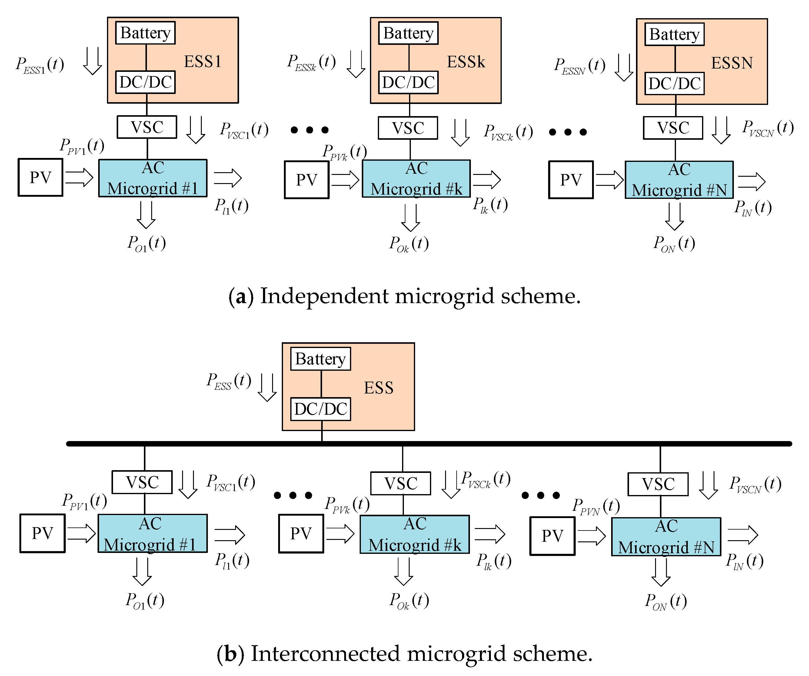
As shown in Figure 7, distributed ESSs are adopted in Case A for the microgrids separately. Through coordinated control of PV generation, loads and ESS, the microgrid net powers can be effectively smoothed, and as a result, the microgrids can be integrated into the upper-level grid with acceptable power fluctuation rates. The capacity of the distributed ESS in the independent microgrid scheme can be sized using the DFT with DFLPF method. With Objective 1 in effect, the expected net powers and the corresponding ESS power curves of microgrid 1–3 are given in Figure 9a–c, respectively. The ESS capacities of the independent microgrid scheme considering Objective 1 are calculated using the sizing algorithm and listed in

Table 2. ESS capacity of independent microgrid scheme with Objective 1.

ESS Capacity	Microgrid 1	Microgrid 2	Microgrid 3
Power Capacity	117 kW	108 kW	127 kW
Energy Capacity	18 kWh	22 kWh	21 kWh

.

As shown in Figure 7, in Case B, a single ESS is connected to the common DC bus shared by the participating microgrids. With the earlier-described fluctuation sharing control applied among the microgrids, the net power fluctuations can be smoothed, and therefore these microgrids can be integrated into the upper-level grid with acceptable fluctuation rates. With Objective 1 in effect, Figure 9d–f show the expected net powers and the corresponding ESS power curves of microgrids, respectively. Using the earlier described ESS sizing algorithm, ESS capacities of interconnected microgrid scheme considering Objective 1 are calculated and listed in

Table 3. ESS capacity of interconnected microgrid scheme with Objective 1.

ESS Capacity	Microgrid 1	Microgrid 2	Microgrid 3
Power Capacity	40 kW	74 kW	54 kW
Energy Capacity	3.2 kWh	5.7 kWh	4.7 kWh

.

Additionally, in the interconnected microgrid scheme, the PCS consists of one DC/DC and three DC/AC converters. The capacity of the DC/DC converter equals the power capacity of the ESS. For the DC/AC converters, since they need to both transfer the ESS power and exchange power among the microgrids, the power capacity is determined by the maximum possible total power flowing through the converters.

6.2. Results Base on Objective 2

To further verify the effectiveness of the interconnected microgrid scheme, the power smoothing results based on Objective 2 are compared using the same method.

In Case A, the expected net powers and the corresponding ESS power curves of independent microgrid 1–3 are shown in Figure 10a–c, respectively. And the ESS capacities considering objective 2 are calculated and listed in

Table 4. ESS capacity of independent microgrid scheme with Objective 2.

ESS Capacity	Microgrid 1	Microgrid 2	Microgrid 3
Power Capacity	190 kW	180 kW	210 kW
Energy Capacity	130 kWh	234 kWh	131 kWh

.

In Case B, the expected net powers and the corresponding ESS power curves of interconnected microgrid 1–3 are shown in Figure 10d–f, respectively. And the ESS capacities considering Objective 2 are calculated and listed in

Table 5. ESS capacity of interconnected microgrid scheme with Objective 2.

ESS Capacity	Microgrid 1	Microgrid 2	Microgrid 3
Power Capacity	80 kW	119 kW	110 kW
Energy Capacity	72 kWh	85 kWh	70 kWh

.

6.3. Results Discussion

The results of the two cases under the different schemes are listed in

Table 6. Results of total ESS and PCS capacity configuration of different schemes.

Objective		Total ESS		DC/DC	DC/AC
		Power Capacity	Energy Capacity
F1min ≤ 5%	Case A	352 kW	61 kWh	352 kW	352 kW
	Case B	90 kW	12 kWh	90 kW	423 kW
F20min ≤ 10%	Case A	580 kW	495 kWh	580 kW	580 kW
	Case B	235 kW	205 kWh	235 kW	659 kW

. Considering that the integrated ESS can provide power for all three microgrids, the total power and energy capacity can be reduced further than the simple addition of the capacities of the distributed ESSs. With the interconnected microgrids and flexible power control, the total power and energy capacities of ESS can be both optimized while meeting the requirement of power fluctuation. With Objective 1 in effect, the total ESS power capacity is reduced from 352 kW to 90 kW, whereas the total energy capacity of the ESS is reduced from 61 kWh to 12 kWh.

In terms of PCS capacity, the DC/DC converter capacity can be optimized under the interconnected scheme thanks to the reduction of ESS power capacity. However, the DC/AC converter capacity increases from 352 kW to 423 kW, an increase which is mainly caused by the power exchanging among multiple microgrids.

The results of the two cases with Objective 2 in effect are also given in the table. As compared with the independent microgrid scheme, the interconnected scheme is also effective for the power fluctuation mitigation in a long-time scale. The total power capacity of the ESS is reduced from 580 kW to 235 kW, whereas the total energy capacity of the ESS is reduced from 495 kWh to 205 kWh. In terms of PCS capacity, the result is similar to that with Objective 1. The DC/DC converter capacity can be optimized under the interconnected scheme, while the capacity of the DC/AC converter increases from 580 kW to 659 kW.

The following conclusions can be drawn from the results given above:

• In a short time scale, power fluctuation mitigation should be based on the ESS power capacity, whereas for a long-time scale, it should be based on both the power and energy capacities of the ESS.
• The proposed interconnection scheme can share fluctuation among participating microgrids and smoothen the total power curve. As a result, both the power and energy capacities of the ESS can be largely optimized under different power fluctuation mitigation objectives.
• The interconnected microgrid scheme with the fluctuation sharing control strategy needs a slight increase in the DC/AC converter capacity because of the extra power exchanging among different microgrids. This may also lead to additional power losses.

6.4. Economic Analysis

Using the flexible multi-microgrid interconnection scheme, the storage and DC-DC converter capacities can be optimized, however at the cost of increased capacities on the AC-DC converter, required DC cable construction, and additional DC power loss. It is therefore necessary to carry out an economic analysis to reveal the true applicability of this method in practical applications. The data in Objective 2 is used to make the economic analysis.

A few assumptions should be made before the economic calculation:

• A lithium-ion battery is used for energy storage in our case, because of its high energy density and lightweight properties [30].
• The voltage level of DC common bus is selected as 750 V. According to Reference [31], 400 V, 750 V and 1500 V voltage levels could be used for DC microgrid construction. In our case study, considering the 380V AC microgrid and the modulation ratio limit of VSC, 750V DC voltage is the best option.
• The calculation cycle of economic analysis is set as 10 years, which is the same as the life cycle of power converters [32]. However, for energy storage, the life cycle is determined by its SOC and charging cycle times. When the lifetime of energy storage is less than 10 years, it is necessary to put in a new battery [33].
• Operational and maintenance costs are neglected in this economic analysis. Both the independent and interconnected schemes need the operational and maintenance cost for converters and storages, and there are no significant differences.
• Each day has the same PV and load power data.

1. The benefits of storage capacity optimization:

The life cycle of storage should be calculated first to determine the change times of batteries in 10 years. The charging times of storage in one day is calculated as:

$$T_{\mathrm{charge}}=\frac{{\displaystyle {\int }_{\mathrm{oneday}}{P}_{\mathrm{charge}}dt}}{E_{ess}\cdot \left(SO{C}_{up}-SO{C}_{low}\right)}$$

(32)

In Equation (32), $T_{\mathrm{charge}}$ is the charging times of storage in one day. $P_{\mathrm{charge}}$ is the charging power of storage in a time interval. ${\displaystyle {\int }_{\mathrm{oneday}}{P}_{\mathrm{charge}}dt}$ is the total charging energy of storage in one day. $E_{ess}$ is the energy capacity of energy storage. $SO{C}_{up}$ and $SO{C}_{low}$ are the upper and lower limits of the SOC, which is the same as Equation (31), and for a better life expectancy, over-discharge should be avoided, thus the maximum SOC is considered as 1, and the minimum SOC is considered as 0.2.

The charging cycle times of lithium-ion battery is 3600 [34]. Therefore, the lifetime of storage is calculated as

$$L=\frac{3600}{T_{\mathrm{charge}}\cdot 365}$$

(33)

In Equation (33), $L$ is the lifetime of storage. Based on the results of Objective 2, the lifetime of storage in different schemes are listed in

Table 7. Lifetime determination of storage in different scheme.

Storage	Independent Scheme			Interconnected Scheme
	Storage of Microgrid 1	Storage of Microgrid 2	Storage of Microgrid 3	Storage in DC Bus
Energy capacity	130 kWh	234 kWh	131 kWh	205 kWh
${\displaystyle {\int }_{\mathrm{oneday}}{P}_{\mathrm{charge}}dt}$	284 kWh	480 kWh	270 kWh	452 kWh
Lifetime (year)	3.6	3.8	3.8	3.6

.

As seen from the table, compared with the independent scheme, the total storage charging power per day is reduced in the interconnected scheme, but the energy capacity of storage is also reduced, thus the lifetimes of storage in different schemes are similar. Therefore, in the time scale of 10 years, batteries need to be replaced twice.

The benefit of storage is calculated as:

$$C_{\mathrm{ESS}}=3\cdot {\mathsf{\Delta }\mathrm{E}}_{\mathrm{ESS}}\cdot c_{\mathrm{ESS}}$$

(34)

In Equation (34), $C_{\mathrm{ESS}}$ is the total benefit of storage optimizing; $\mathsf{\Delta }{\mathrm{E}}_{\mathrm{ESS}}$ is the saved energy capacity of the ESS; $c_{\mathrm{ESS}}$ is the unit price of the ESS.

2. The benefits and costs of power converters:

In the interconnected scheme, the DC-DC converter capacities can be reduced at the cost of increased capacities on the AC-DC converter, which is calculated as:

$$C_{conv}=\mathsf{\Delta }{S}_{DC-DC}\cdot c_{DC-DC}-\mathsf{\Delta }{S}_{AC-DC}\cdot c_{AC-DC}$$

(35)

In Equation (35), $C_{\mathrm{ESS}}$ is the total benefit of power converter capacities optimization; $\mathsf{\Delta }{S}_{DC-DC}$ is the saved power capacity of DC-DC converter; $c_{DC-DC}$ is the unit price of DC-DC; $\mathsf{\Delta }{S}_{AC-DC}$ is the extra power capacity requirement of AC-DC converter; $c_{AC-DC}$ is the unit price of AC-DC.

3. The costs of DC-line

Extra DC-line cost is needed in the interconnected scheme, including construction cost and power loss cost. The DC-line cost is calculated as:

$$C_{line}=l\cdot c_{line}+{\displaystyle \int i_{DC}^2(t)r_{dc}ldt\cdot c_E}$$

(36)

In Equation (36), $C_{line}$ is the total cost of DC-line, $l$ is the DC line length; $c_{line}$ is the unit price of DC line; $i_{DC}(t)$ is the power transfer current in DC line; $r_{DC}$ is the unit length resistance; $c_E$ is the average unit electricity price.

With a prescribed DC voltage, the maximum transfer DC current can be calculated, and the DC cable parameters can be determined. The unit length resistance and unit price of the DC-line can then be calculated accordingly. This process is expressed as:

$$\begin{array}{l}{I}_{DC\_\max }=\frac{P_{DC\_\max }}{U_{DC}},S=f_1(I_{DC\_\max }),\\ c_{line}=f_2(S),r_{DC}=\rho /S\end{array}$$

(37)

In Equation (37), $P_{DC\_\max }$ is the maximum DC transfer power, $U_{DC}$ is the DC line voltage, $I_{DC\_\max }$ is the maximum DC transfer current, $S$ is the cross-section area of the DC cable, and $\rho$ is the copper resistivity of the DC cable. The functions $f_1$ and $f_2$ relating $I_{DC\_\max }$, $S$ and $C_{DC\_Line}$ are given by the DC cable manufacturers.

According to Equations (32)–(37), the total revenue of the interconnected scheme is

$$R=3\cdot \mathsf{\Delta }{E}_{\mathrm{ESS}}\cdot c_{\mathrm{ESS}}+\mathsf{\Delta }{S}_{DC-DC}\cdot c_{DC-DC}-\mathsf{\Delta }{S}_{AC-DC}\cdot c_{AC-DC}-l\cdot c_{line}-{\displaystyle \int i_{DC}^2(t)r_{DC}ldt}\cdot c_E$$

(38)

Based on Equation (38), and the constant parameters given in

Table 8. Constant parameters used for economic analysis.

Parameter	${\mathit{c}}_{\mathbf{ESS}}$	${\mathit{c}}_{\mathit{D}\mathit{C}-\mathit{D}\mathit{C}}$	${\mathit{c}}_{\mathit{A}\mathit{C}-\mathit{D}\mathit{C}}$	$\mathit{\rho }$	${\mathit{c}}_{\mathit{E}}$
Unit	$/kWh	$/kW	$/kW	Ω·mm2/m	$/kWh
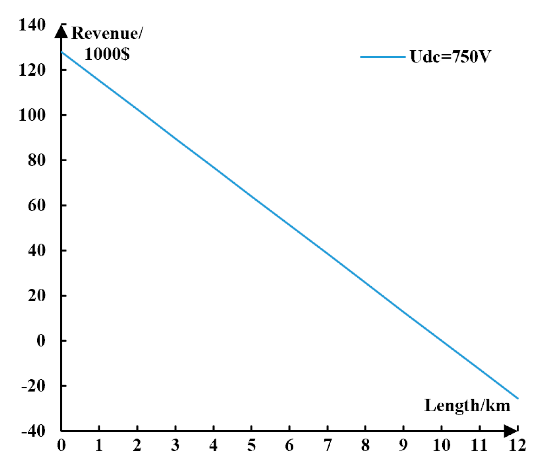
Price	416	73	105	0.0217	0.12

, the result of economic analysis with different DC line lengths is given in Figure 11.

In Figure 11, it is shown that the DC line length needs to be restricted for avoiding massive investment in DC cable. In this case, as long as the microgrids distance is less than 10 km, DC interconnection and ESS optimization design will have positive revenue. Therefore, the proposed scheme is most suitable for industrial parks and urban commercial areas where the distances between microgrids are short, but may not be suitable for remote area applications where the distances are too long for DC line construction.

7. Conclusions

Based on the above analysis, conclusions of this paper are listed below.

1. A new multi-microgrid interconnection scheme is proposed to optimize the capacities of ESS used in microgrids to mitigate power fluctuations. By adopting a fluctuation sharing control strategy among the participating microgrids, the effectiveness of power fluctuation mitigation with the proposed scheme is analyzed.

2. Using the control strategy of VSCs and DFT plus DFLPF method for sizing of the ESS capacity, the cases of the independent microgrid scheme and the interconnected microgrid scheme are studied and compared in detail. It is shown that, as compared with the traditional implementation of independent microgrids, linking them together through a common DC bus can effectively help with the optimization of the ESS capacities.

3. Using the flexible multi-microgrid interconnection scheme, the storage and DC-DC converter capacities can be optimized, however at the cost of increased capacities on the AC-DC converter, required DC cable construction, and additional DC power loss. Based on the economic analysis, the DC line length will influence the proposed scheme benefits significantly. The interconnected scheme is most suitable for urban microgrids where the distance among them is short.

In fact, not only can microgrid interconnection mitigate power fluctuations, it can help with load balancing, distribution transformer capacity optimization, power quality improvement as well. Future work will concentrate on developing advanced functions of the interconnected scheme to maximize the scheme’s benefits.

References

1. Katiraei, F.; Aguero, J.R. Solar PV Integration Challenges. IEEE Power Energy Mag. 2011, 9, 62–71. [Google Scholar] [CrossRef]
2. Bebic, J.; Walling, R.; O’Brien, K.; Kroposki, B. The sun also rises. IEEE Power Energy Mag. 2009, 7, 45–51. [Google Scholar]
3. Ralph, M.; Ellis, A.; Borneo, D.; Corey, G.; Baldwin, S. Transmission and distribution deferment using PV and energy storage. In Proceedings of the 2011 37th IEEE Photovoltaic Specialists Conference, Seattle, WA, USA, 19–24 June 2011. [Google Scholar]
4. Pan, W.X.; Liu, M.Y.; Feng, B. An analysis of battery demand capacity of wind/storage system and control of state of charge. In Proceedings of the International Conference on Renewable Power Generation (RPG 2015), Beijing, China, 17–18 October 2015. [Google Scholar]
5. Haan, J.E.S.D.; Frunt, J.; Kling, W.L. Mitigation of wind power fluctuations in smart grids. In Proceedings of the 2010 IEEE PES Innovative Smart Grid Technologies Conference Europe (ISGT Europe), Gothenberg, Sweden, 11–13 October 2010. [Google Scholar]
6. Macdougall, P.; Warmer, C.; Kok, K. Mitigation of wind power fluctuations by intelligent response of demand and distributed generation. In Proceedings of the 2011 2nd IEEE PES International Conference and Exhibition on Innovative Smart Grid Technologies, Manchester, UK, 5–7 December 2011. [Google Scholar]
7. Steffel, S.; Dinkel, A. Absorbing the Rays. IEEE Power Energy Mag. 2013, 11, 45–54. [Google Scholar] [CrossRef]
8. Bass, R.B.; Carr, J.; Aguilar, J.; Whitener, K. Determining the Power and Energy Capacities of a Battery Energy Storage System to Accommodate High Photovoltaic Penetration on a Distribution Feeder. IEEE Power Energy Technol. Syst. J. 2016, 3, 119–127. [Google Scholar] [CrossRef] [Green Version]
9. Chen, S.X.; Gooi, H.B.; Wang, M.Q. Sizing of Energy Storage for Microgrids. IEEE Trans. Smart Grid 2012, 3, 142–151. [Google Scholar] [CrossRef]
10. Malik, S.M.; Ai, X.; Sun, Y.; Chen, Z.; Zhou, S. Voltage and frequency control strategies of hybrid AC/DC microgrid: A review. IET Gener. Transm. Distrib. 2017, 11, 303–313. [Google Scholar] [CrossRef]
11. Lasseter R, H. MicroGrids. In Proceedings of the Power Engineering Society Winter Meeting, New York, NY, USA, 27–31 January 2002. [Google Scholar]
12. Yoshimoto, K.; Nanahara, T.; Koshimizu, G. Analysis of data obtained in demonstration test about battery energy storage system to mitigate output fluctuation of wind farm. In Proceedings of the Integration of Wide-Scale Renewable Resources into the Power Delivery System, Calgary, AB, Canada, 29–31 July 2009. [Google Scholar]
13. Liu, B.; Zhuo, F.; Zhu, Y.; Yi, H. System Operation and Energy Management of a Renewable Energy-Based DC Micro-Grid for High Penetration Depth Application. IEEE Trans. Smart Grid 2015, 6, 1147–1155. [Google Scholar] [CrossRef]
14. Jiang, Q.; Wang, H. Two-Time-Scale Coordination Control for a Battery Energy Storage System to Mitigate Wind Power Fluctuations. IEEE Trans. Energy Convers. 2013, 28, 52–61. [Google Scholar] [CrossRef]
15. Alam, M.J.E.; Muttaqi, K.M.; Sutanto, D. A Novel Approach for Ramp-Rate Control of Solar PV Using Energy Storage to Mitigate Output Fluctuations Caused by Cloud Passing. IEEE Trans. Energy Convers. 2014, 29, 507–518. [Google Scholar]
16. Nykvist, B.; Nilsson, M. Rapidly falling costs of battery packs for electric vehicles. Nat. Clim. Chang. 2015, 5, 329–332. [Google Scholar] [CrossRef]
17. Zamora, R.; Srivastava, A.K. Multi-Layer Architecture for Voltage and Frequency Control in Networked Microgrids. IEEE Trans. Smart Grid 2016, 9, 2076–2085. [Google Scholar] [CrossRef]
18. Xia, Y.; Wei, W.; Yu, M.; Peng, Y.; Tang, J. Decentralized Multi-Time Scale Power Control for a Hybrid AC/DC Microgrid with Multiple Subgrids. IEEE Trans. Power Electron. 2017, 33, 4061–4072. [Google Scholar] [CrossRef]
19. Xia, Y.; Wei, W.; Yu, M.; Wang, X.; Peng, Y. Power Management for a Hybrid AC/DC Microgrid with Multiple Subgrids. IEEE Trans. Power Electron. 2017, 33, 3520–3533. [Google Scholar] [CrossRef]
20. Zhou, J.; Zhang, J.; Cai, X.; Li, Z.; Wang, J.; Zang, J. A Novel Flexible Interconnection Scheme for Microgrid to Optimize the Capacity of Energy Storage System (ESS). In Proceedings of the 2018 International Power Electronics Conference, Niigata, Japan, 20–24 May 2018. [Google Scholar]
21. Alam, M.J.E.; Muttaqi, K.M.; Sutanto, D. Distributed energy storage for mitigation of voltage-rise impact caused by rooftop solar PV. In Proceedings of the 2012 IEEE Power and Energy Society General Meeting, San Diego, CA, USA, 22–26 July 2012; pp. 1–8. [Google Scholar]
22. Yang, T. The optimal capacity determination method of energy storage system with different applications in wind farm. In Proceedings of the 2016 IEEE PES Asia-Pacific Power and Energy Engineering Conference (APPEEC), Xi’an, China, 25–28 October 2016; pp. 2081–2085. [Google Scholar]
23. Jamali, A.A.; Nor, N.M.; Ibrahim, T. Energy storage systems and their sizing techniques in power system—A review. In Proceedings of the 2015 IEEE Conference on Energy Conversion (CENCON), Johor Bahru, Malaysia, 19–20 October 2015; pp. 215–220. [Google Scholar]
24. Ogimi, K.; Yoza, A.; Yonama, A. A study on optimum capacity of battery energy storage system for wind farm operation with wind power forecast data. In Proceedings of the 2012 IEEE 15th International Conference on Harmonics and Quality of Power, Hong Kong, China, 17–20 June 2012; pp. 118–123. [Google Scholar]
25. Barton, J.P.; Infield, D.G. Energy storage and its use with intermittent renewable energy. IEEE Trans. Energy Convers. 2004, 19, 441–448. [Google Scholar] [CrossRef]
26. Moon, S.-P.; Kim, S.-Y.; Labios, R.; Yoon, Y.-B. Determining wind farm locations, allocation of wind farm capacity, and sizing of energy storage for 17 GW new wind power capacity in Korea. In Proceedings of the 2016 IEEE Power and Energy Society General Meeting (PESGM), Boston, MA, USA, 17–21 July 2016. [Google Scholar]
27. Xiao, J.; Bai, L.; Li, F.; Liang, H.; Wang, C. Sizing of Energy Storage and Diesel Generators in an Isolated Microgrid Using Discrete Fourier Transform (DFT). IEEE Trans. Sustain. Energy 2014, 5, 907–916. [Google Scholar] [CrossRef]
28. Wang, X.Y.; Vilathgamuwa, D.M.; Choi, S.S. Determination of Battery Storage Capacity in Energy Buffer for Wind Farm. IEEE Trans. Energy Convers. 2008, 23, 868–878. [Google Scholar] [CrossRef]
29. Cao, M.; Xu, Q.; Bian, H.; Yuan, X.; Du, P. Research on configuration strategy for regional energy storage system based on three typical filtering methods. IET Gener. Transm. Distrib. 2016, 10, 2360–2366. [Google Scholar] [CrossRef]
30. Hannan, M.A.; Hoque, M.M.; Hussain, A.; Yusof, Y.; Ker, P.J. State-of-the-Art and Energy Management System of Lithium-Ion Batteries in Electric Vehicle Applications: Issues and Recommendations. IEEE Access 2018. [Google Scholar] [CrossRef]
31. Rodriguez-Diaz, E.; Chen, F.; Vasquez, J.C.; Guerrero, J.M.; Burgos, R.; Boroyevich, D. Voltage-Level Selection of Future Two-Level LVdc Distribution Grids. IEEE Electrif. Mag. 2016, 4, 20–28. [Google Scholar] [CrossRef]
32. Mukherjee, N.; Strickland, D. Analysis and Comparative Study of Different Converter Modes in Modular Second Life Hybrid Battery Energy Storage Systems. IEEE J. Emerg. Sel. Top. Power Electron. 2015, 4, 547–563. [Google Scholar] [CrossRef]
33. Ayeng’o, S.P.; Schirmer, T.; Kairies, K.P.; Axelsen, H.; Sauer, D.U. Comparison of off-grid power supply systems using lead-acid and lithium-ion batteries. Sol. Energy 2018, 162, 140–152. [Google Scholar] [CrossRef]
34. Lin, S.; Wang, Z. Economic analysis of energy storage systems invested by a power supply bureau. Electr. Eng. 2019, 7, 28–32. [Google Scholar]
Figure 1. Configuration of the flexible multi-microgrid interconnection scheme.
Energies 12 02132 g001
Figure 2. Active power flow for power fluctuation analysis.
Energies 12 02132 g002
Figure 3. Power converter topologies of the multi-microgrid interconnection scheme.
Energies 12 02132 g003
Figure 4. The control diagram of VSC-k.
Energies 12 02132 g004
Figure 5. Control diagram of the DC-DC converter.
Energies 12 02132 g005
Figure 6. Procedure of ESS capacity sizing.
Energies 12 02132 g006
Figure 7. Microgrid configurations for the case study.
Energies 12 02132 g007
Figure 8. Net power curves of the independent feeders without ESS.
Energies 12 02132 g008
Figure 9. Microgrid original power (yellow line), expected power (grey line) and ESS power (blue line) curve based on Objective 1. (a) Results of independent microgrid 1. (b) Results of independent microgrid 2. (c) Results of independent microgrid 3. (d) Results of interconnected microgrid 1. (e) Results of interconnected microgrid 2. (f) Results of interconnected microgrid 3.
Energies 12 02132 g009
Figure 10. Microgrid original power (yellow line), expected power (grey line) and ESS power (blue line) curve based on Objective 2. (a) Results of independent microgrid 1. (b) Results of independent microgrid 2. (c) Results of independent microgrid 3. (d) Results of interconnected microgrid 1. (e) Results of interconnected microgrid 2. (f) Results of interconnected microgrid 3.
Energies 12 02132 g010
Figure 11. Total revenue with different DC line length.
Energies 12 02132 g011