A Method to Enhance the Global Efficiency of High-Power Photovoltaic Inverters Connected in Parallel

Abstract

Central inverters are usually employed in large photovoltaic farms because they offer a good compromise between costs and efficiency. However, inverters based on a single power stage have poor efficiency in the low power range, when the irradiation conditions are low. For that reason, an extended solution has been the parallel connection of several inverter modules that manage a fraction of the full power. Besides other benefits, this power architecture can improve the efficiency of the whole system by connecting or disconnecting the modules depending on the amount of managed power. In this work, a control technique is proposed that maximizes the global efficiency of this kind of systems. The developed algorithm uses a functional model of the inverters’ efficiency to decide the number of modules on stream. This model takes into account both the power that is instantaneously processed and the maximum power point tracking (MPPT) voltage that is applied to the photovoltaic field. A comparative study of several models of efficiency for photovoltaic inverters is carried out, showing that bidimensional models are the best choice for this kind of systems. The proposed algorithm has been evaluated by considering the real characteristics of commercial inverters, showing that a significant improvement of the global efficiency is obtained at the low power range in the case of sunny days. Moreover, the proposed technique dramatically improves the global efficiency in cloudy days.

1. Introduction

Photovoltaic (PV) generation has had rapid growth in the last years and is now a significant contribution to the renewable sources of electricity [1,2,3,4,5]. With the purpose of improving the profitability of photovoltaic systems, large-scale PV plants are being installed [6]. In large PV plants, low-power decentralized architectures based on string inverters are usually avoided due to their high cost. Therefore, photovoltaic farms are usually connected to the grid through central inverters that manage the whole power of the system, since they offer a good compromise between costs and efficiency [7].

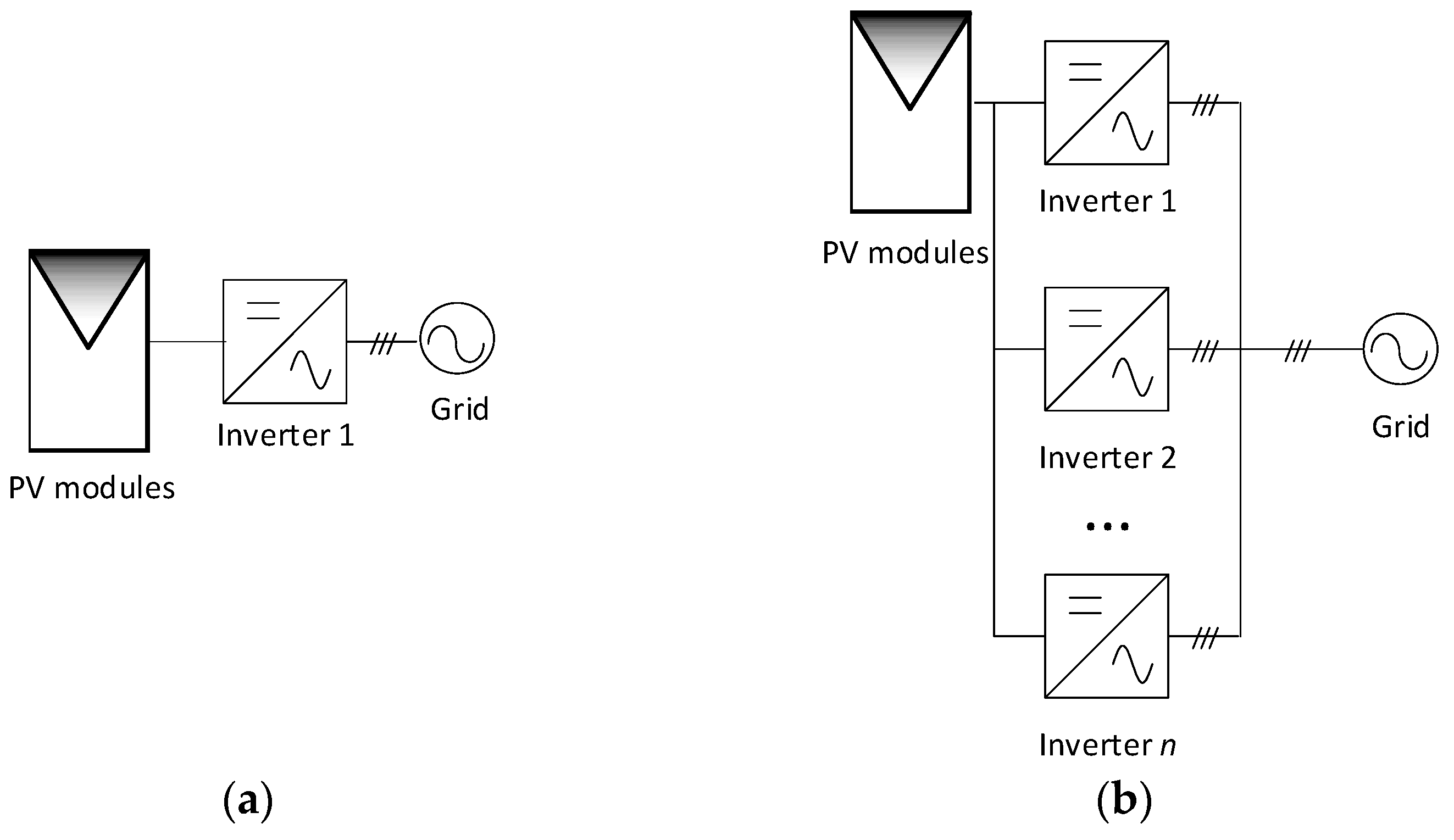
Figure 1 shows two alternatives to build up a centralized inverter that connects a large PV field to the distribution grid. The efficiency of central inverters composed by a single power stage, Figure 1a, is poor in the low power range when the radiation conditions are low. In the range of MWs, the scheme showed by Figure 1b is preferred, as the parallel connection of several modules offers redundancy, scalability, and a certain degree of fault tolerance. A popular technique to manage the connection of paralleled inverters is average current-sharing (CS). CS offers several advantages, such as a good power sharing among the modules and simplicity of implementation. However, the efficiency of the whole system with this technique at low power is not improved with regard to the single-module configuration [6,8].

To overcome this problem, the inverter modules can be connected and disconnected depending on the global delivered power. The concept of connecting/disconnecting the phases of a converter depending on the load-current level has been also applied in several works to low power converters [9,10,11,12,13]. In [9] the phase shedding points are calculated based on a lookup table defined by the junction temperature and on-resistance of MOSFETs. In [10] a multiphase buck converter with a rotating phase-shedding scheme has been presented. In [11] a method is proposed that linearly increases/reduces the power delivered by some channels when the demanded power changes. In [13] a time optimal digital controller for the phase shedding in multiphase buck converters has been developed. Although all these methods are based on the connection/disconnection of phases (or modules) to improve the efficiency of the global system, they cannot be directly extrapolated to high-power inverters.

Some studies regarding the connection/disconnection of paralleled inverters have been developed in the past. In [14] a methodology based on unidimensional efficiency curves and a genetic algorithm was presented. In that work, a unidimensional model is used, so the changes in the maximum power point tracking (MPPT) voltage are not considered. Therefore, this algorithm could be inappropriate in most of the photovoltaic applications. Moreover, the stochastic nature of the genetic algorithm requires the implantation of complex processes to obtain a useful result. This fact could impede the real-time implementation of the technique. In [15], a piecewise curve fitting is used to define the efficiency function and an artificial-intelligence-based algorithm is implemented to obtain the optimized current-sharing. As in [15], a unidimensional model is used to calculate the efficiency of the inverter, and the algorithm proposes a random initialization that requires many iterations to obtain a valid result. Finally, in [16], each converter regulates its respective output power following an algorithm of prioritization. However, the algorithm improves the efficiency in the low range of power but worsens the efficiency in the middle and high power range.

Regarding the efficiency of inverters, there are several efficiency models for photovoltaic inverters that have been proposed in the literature. These models can be classified as unidimensional and bidimensional, depending on whether they only take into account the generated power, or if they consider both the power generation and the DC voltage at the input of the inverter. Some unidimensional and bidimensional models were studied in [17,18,19,20,21,22,23,24,25].

In this work, a control technique is proposed that decides, in real time conditions, the proper number of inverters that should be on stream to improve the global efficiency in the whole power range. The developed algorithm is based on a bidimensional model of the inverters’ efficiency, which takes into account not only the amount of delivered power but also the value of the DC voltage at the input of the inverters, which is continuously changing to achieve the maximum power point (MPP) of the PV field. The algorithm calculates the efficiency of the whole power system by taking into account various scenarios and selects the one that offers the best instantaneous efficiency. A comparative study of the model’s accuracy has also been carried out by considering data of several commercial inverters. Data have been obtained from the “Grid Support Inverters List” published by the California Energy Commission [26]. However, it is worth noting that the parameters could be easily extracted from the datasheet of manufacturers, or obtained by means of a reduced number of efficiency measurements on the inverter.

The main contributions of this paper are the following:

• A comparative study of the advantages and limitations of various models of efficiency for photovoltaic inverters.
• The proposal of an algorithm that decides the number of inverter modules that should be on stream to obtain the maximum efficiency of the global system in the whole operation range. An advantage of the proposed algorithm is the low requirements in terms of computational resources so that it can be easily implemented in a real time operation.
• A detailed study of the expected performance of the proposed algorithm when it is applied to several commercial photovoltaic inverters.

2. Efficiency Modeling of PV Inverters

As it has been pointed out in the previous section, two kinds of functional models have been proposed in the literature to evaluate the efficiency of power inverters: unidimensional, in which only the generated power is considered, and bidimensional, in which takes into account both the generated power and the DC voltage at the input of the inverter, which agrees with the MPPT voltage in the case of central inverters.

2.1. Unidimensional Models

The unidimensional model of Jantsch [17,18,19] is expressed by (1), where k₀, k₁, and k₂ are the coefficients to be calculated for any inverter, and c is the load factor, which is defined as the ratio between the power that is processed at a certain instant and the nominal power of the inverter. In (1), the part of the losses that are independent of the generated power (constant losses) are weighted by k₀, the losses that linearly depend on the load factor are weighted by k₁ and the losses with a quadratic dependence on the load factor are weighted by k₂.

$$\eta \left(c\right)=\frac{c}{c+\left(k_0+k_{1}c+k_2{c}^2\right)}$$

(1)

Dupont [20] indicates that the efficiency of power inverters can be approximated by the second order function (2), being α₁, α₀, β₁, and β₀ coefficients that can be obtained by applying curve fitting algorithms over experimental measurements and c is the load factor of the inverter.

$$\eta \left(c\right)=\frac{{\propto }_{1}c+{\propto }_0}{c^2+{\beta }_{1}c+{\beta }_0}$$

(2)

2.2. Bidimensional Models

In photovoltaic inverters that are directly connected to the PV field, as is the case of central inverters, the DC input voltage of the inverters is continuously following the operation point that is calculated by the maximum power point tracking (MPPT) algorithm. Therefore, the use of unidimensional models that consider the DC voltage as constant is inappropriate to properly evaluate the actual efficiency of the inverter in the whole operation range. To overcome this problem, several bidimensional models have been proposed.

Rampinelli [23] modifies the model represented by (1), which only considers the efficiency as a function of the delivered power, by taking also into account the influence of the input voltage on the predicted efficiency. To achieve this, the coefficients k₀, k₁, and k₂ are expressed as a function of the input voltage being modified as k₀′_(vin), k₁′_(vin), and k₂′_(vin). The expressions of these coefficients are defined as (3)–(5), by assuming that the coefficients have a linear dependency with the input voltage and k_0,0, k_0,1, k_1,0, k_1,1, k_2,0, and k_2,1 are the coefficients to be calculated. This modeling approach is described by (6).

$$k_0^{\prime }\left(v_{in}\right)=K_{0,0}+k_{0,1}{v}_{in}$$

(3)

$$k_1^{\prime }\left(v_{in}\right)=K_{1,0}+k_{1,1}{v}_{in}$$

(4)

$$k_2^{\prime }\left(v_{in}\right)=K_{2,0}+k_{2,1}{v}_{in}$$

(5)

$$\eta \left(c,v_{in}\right)=\frac{c}{c+\left(k_0^{\prime }\left(v_{in}\right)+k_1^{\prime }\left(v_{in}\right)c+k_2^{\prime }\left(v_{in}\right)c^2\right)}$$

(6)

Similarly, if it is assumed that the efficiency can vary in a quadratic way regarding both the delivered power and the DC voltage, the coefficients can be calculated as (7)–(9). As a result, Equation (10) describes a model of the inverter that considers a nonlinear dependency with the input voltage.

$$k_0^{″}\left(v_{in}\right)=K_{0,0}+k_{0,1}{v}_{in}+k_{0,2}{v}_{in}^2$$

(7)

$$k_1^{″}\left(v_{in}\right)=K_{1,0}+k_{1,1}{v}_{in}+k_{1,2}{v}_{in}^2$$

(8)

$$k_2^{″}\left(v_{in}\right)=K_{2,0}+k_{2,1}{v}_{in}+k_{2,2}{v}_{in}^2$$

(9)

$$\eta \left(c,v_{in}\right)=\frac{c}{c+\left(k_0^{″}\left(v_{in}\right)+k_1^{″}\left(v_{in}\right)c+k_2^{″}\left(v_{in}\right)c^2\right)}$$

(10)

In [24] Sandia Laboratories propose a mathematical model that describes the performance of inverters. The Sandia model is represented in (11)–(14), where pac is the output power of the inverter; p_{ac_o} is the nominal AC power rating, pdc is the input power of the inverter, vdc is the input voltage of the inverter, vdc_o is the nominal DC voltage, pdc_o is the nominal input power, pso is the minimum considered DC power; co is a parameter that defines the curvature of the relationship between AC power and DC power at nominal voltage. Finally, c1, c2, and c3 are coefficients that represent the linear relationship between p_{dc_o}, p_so, and c_o, respectively, and the DC input voltage.

$$A=p_{dc\_o}\left(1+c_1\left(v_{dc}-v_{dc\_o}\right)\right)$$

(11)

$$B=p_{so}\left(1+c_2\left(v_{dc}-v_{dc\_o}\right)\right)$$

(12)

$$C=c_o\left(1+c_3\left(v_{dc}-v_{dc\_o}\right)\right)$$

(13)

$$p_{ac}=\left(\frac{p_{ac\_o}}{A-B}-C\left(A-B\right)\right)\left(p_{dc}-B\right)+C{\left(p_{dc}-B\right)}^2$$

(14)

$$\eta =\frac{p_{ac}}{p_{dc}}$$

(15)

Finally, Driesse [25] proposes a model defined as (16)–(19), with b_0,0…2, b_10…2, b_2,0…2 being the coefficients to be fitted.

$$b_0\left(v_{in}\right)=b_{0,0}+b_{0,1}\left(v_{in}-1\right)+b_{0,2}\left(\frac{1}{v_{in}}-1\right)$$

(16)

$$b_1\left(v_{in}\right)=b_{1,0}+b_{1,1}\left(v_{in}-1\right)+b_{1,2}\left(\frac{1}{v_{in}}-1\right)$$

(17)

$$b_2\left(v_{in}\right)=b_{2,0}+b_{2,1}\left(v_{in}-1\right)+b_{2,2}\left(\frac{1}{v_{in}}-1\right)$$

(18)

$$\eta \left(c,v_{in}\right)=\frac{c}{c+b_0\left(v_{in}\right)+b_1\left(v_{in}\right)c+b_2\left(v_{in}\right)c^2}$$

(19)

3. Description of the Proposed Efficiency Oriented Algorithm

As it was described in the introduction section, the proposed algorithm calculates the optimal number of parallel modules of a central inverter that should be on stream to maximize the global efficiency in the whole power range.

The algorithm is initially based on the calculation of the local maxima by applying the second derivative test to the function that predicts the efficiency of the whole system, eff(c_i, v_in). This function (20) computes the efficiency of the whole system starting from the efficiency of each one of the modules, η(c_i, v_in) that can be obtained by means of one of the functional models that were described in the previous section. In (20), c_i (i = 1, 2, …, n) is the load factor of each parallel inverter, i.e., the ratio between the power that is actually managed by each module and its nominal power. The DC voltage of the central inverter is represented by v_in.

$$eff\left(c_i,v_{in}\right)={\displaystyle \sum }_{i=1}^n\frac{c_i}{c_1+c_2+\dots +c_n}·\eta \left(c_i,v_{in}\right)$$

(20)

To apply the second derivative test, the critical points of the function (20) can be calculated by solving the equations’ system obtained from the first partial derivatives. From the second derivative, the Hessian matrix (21) can be obtained [27]. Finally, if H in a critical point is negative definite, that critical point is a local maximum. Therefore, the optimal load factor for each one of the modules on stream that maximizes the global efficiency can be obtained by solving (20) and (21) for a certain operating point described by both the DC voltage and the supplied power. It is worth pointing out that the second derivative test does not calculate the maxima points when some of c_i = 0. To solve this issue, n different eff_j(c_i, v_in) can be defined, being j = 1…n and i = 1…n. Following this procedure, j relative maximums are obtained, one for each eff_j(c_i, v_in), with the searched maximum being the highest of these.

$$H=\left[\begin{array}{ccc}\frac{{\partial }^{2}eff}{\partial c_1^2}& \dots & \frac{{\partial }^{2}eff}{\partial c_n{c}_1}\\ ⋮& \ddots & ⋮\\ \frac{{\partial }^{2}eff}{\partial c_1{c}_n}& \dots & \frac{{\partial }^{2}eff}{\partial c_n{c}_n}\end{array}\right]$$

(21)

One disadvantage of this procedure is the very high computation time needed to calculate all the critical points for a large set of c_i values. However, all the local maximums for a certain eff_j(c_i, v_in) are produced when the power is equally shared among the modules, i.e., c₁ = c₂ … = c_n. Therefore, the method can be simplified since only the number of modules on stream that maximizes the global efficiency should be calculated. By applying this condition, a practical implementation of the proposed method can be obtained, which is shown in the following section.

Practical Implementation of the Proposed Efficiency Oriented Algorithm

Starting from the predictions of a functional model of inverters efficiency, the algorithm calculates the efficiency of the central inverter by considering all possible combinations of modules on stream and chooses the result that offers the maximum efficiency. As it has been highlighted before, the relative maximum values of efficiency are achieved when the power is equally shared among the modules, so it should be calculated only the value of n that maximizes the global efficiency. One of the most important characteristics of the simplified algorithm is the low need for computational resources and its easy implementation to work in real time conditions.

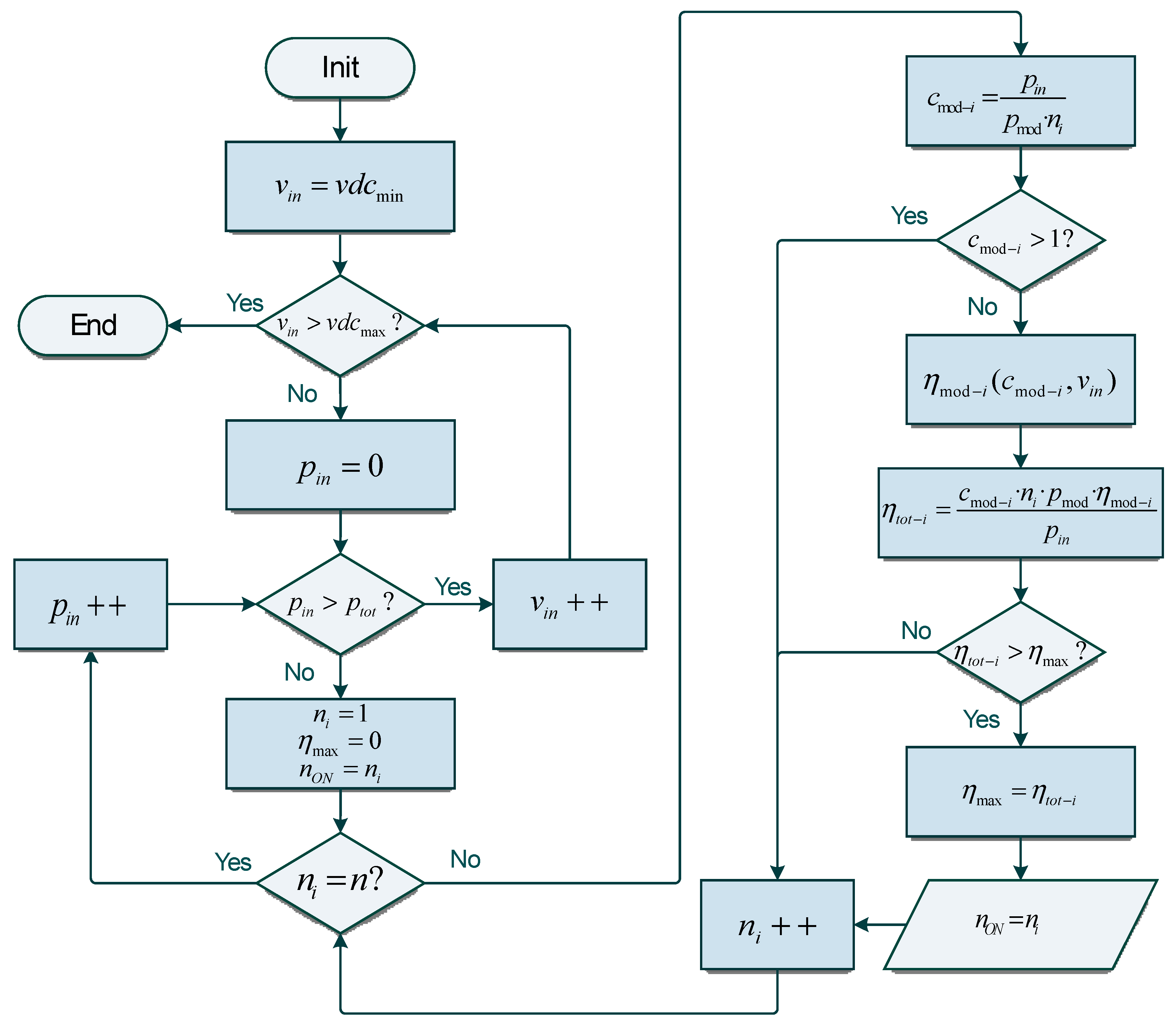
Figure 2 shows the flowchart of the proposed algorithm. In the figure, v_in and p_in are the MPPT input voltage and the generated power, respectively, while vdc_min and vdc_max are the limits of the MPP voltage range of the inverter. The nominal power of the photovoltaic farm and the one of each parallel inverter are represented by p_tot and p_mod, respectively; n is the total number of parallel modules; n_i, c_mod-i, c_tot-i, η_mod-I, and η_tot-i (for i = 1 to n) represent the number of inverters considered in each iteration, the load factor of only a module, the load factor of the whole system, the efficiency of each module and the one of the whole system, respectively, in all cases for the corresponding iteration. Finally, n_ON is the number of modules on stream that achieves the global maximum efficiency η_max.

4. Methods

4.1. Selection of Inverters for the Study

Table 1. List of inverters under study (Source: CEC (California Energy Commission) Grid Support Inverters List).

Number of Inverter	Inverter	Company	Nominal Power
1	MPS-250HV	Dynapower	250 kW
2	EQX0250UV480TN	Perfect Galaxy International Ltd.	250 kW
3	FS0501CU	Power Electronics	500 kW
4	IF500TL-UL OUTDOOR	Jema Energy	500 kW
5	XP500U-TL	KACO new energy	500 kW
6	EQMX0500UV320XP	Perfect Galaxy International Ltd.	500 kW
7	SGI 500XTM	Yaskawa Solectria Solar	500 kW
8	PV-625-XRLS-VV-STG	Perfect Galaxy International Ltd.	625 kW
9	Conext Core XC680-NA	Schneider Electric	680 kW
10	EQX0750UV320XP	Perfect Galaxy International Ltd.	750 kW
11	ULTRA-750-TL-OUTD-4-US	Power-One	750 kW
12	SC750CP-US	SMA America	770 kW
13	ULTRA-750-TL-OUTD-1-US	ABB	780 kW
14	HS-P1000GLO-U	Hyosung Heavy Industries	1 MW
15	ULTRA-1100-TL-OUTD-2-US	ABB	1 MW
16	ULTRA-1100-TL-OUTD-4-US	ABB	1 MW
17	EQX1000UV400XP	Perfect Galaxy International Ltd.	1 MW
18	ULTRA-1100-TL-OUTD-4-US	Power-One	1 MW
19	SG1000MX	Sungrow Power Supply	1 MW
20	FS0900CU	Power Electronics	1 MW

summarizes the commercial inverters that have been evaluated to validate the proposed concepts. The required data to build up the efficiency models of the inverters have been extracted from the “Grid Support Inverters List” that California Energy Commission (CEC) publishes [26].

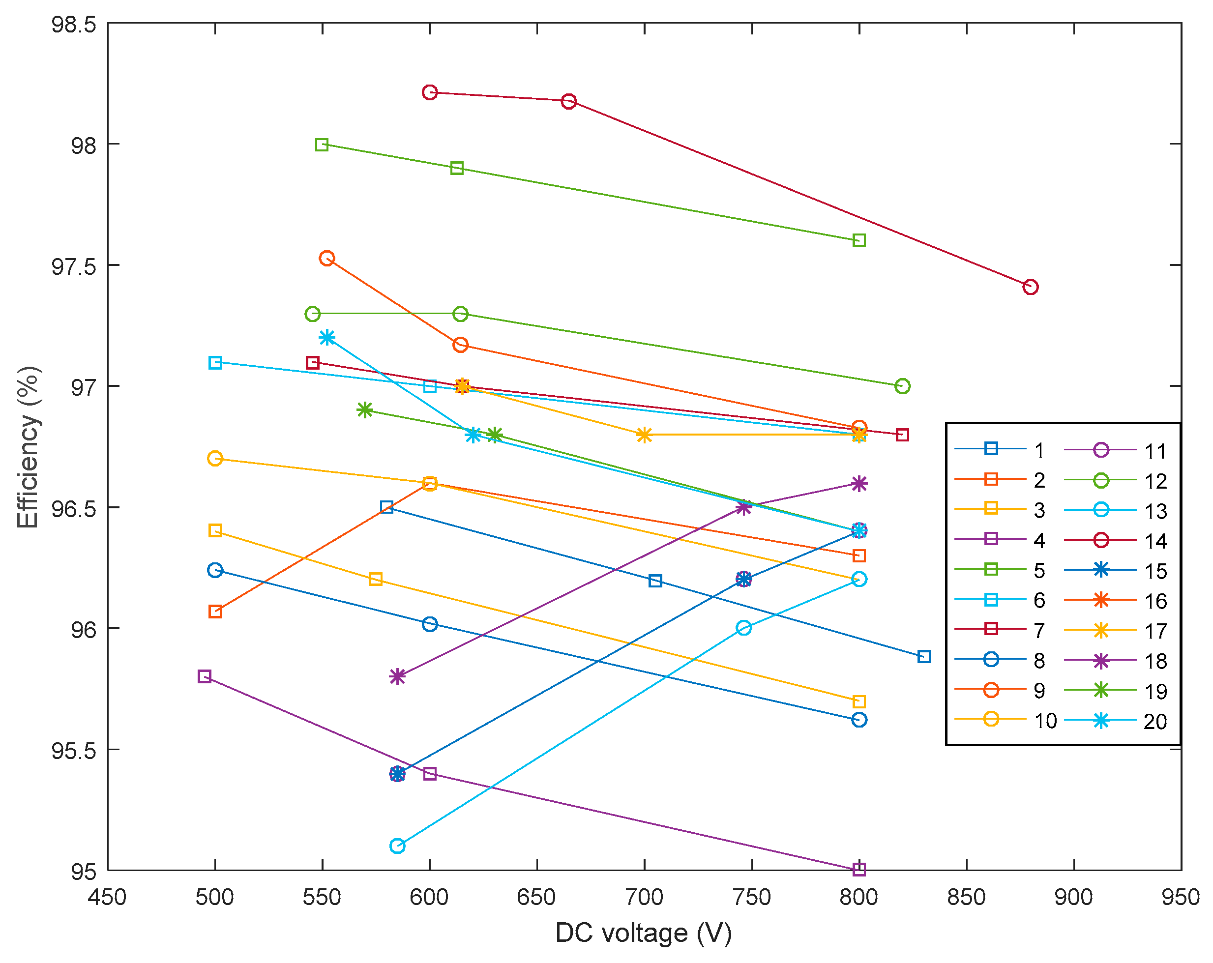
Although the proposed methods have been applied to all the inverters summarized by Table 1, in the following only a selection of the most representative results is shown. To choose those representative results, 3 inverters with significant differences in their respective dependence of the MPP voltage on the inverter efficiency have been considered. In Figure 3, the relationship between the input voltage and the efficiency of the listed inverters has been represented. Note that, in some cases, the curves have an ascendant and nonlinear relationship with the input voltage; in some others, they have a descendant and linear relationship with the voltage and, finally, some curves have a descendant and nonlinear relationship with the voltage.

To consider the three possibilities (categories) of the efficiency dependency regarding the voltage, a sample of each category for the study presented in this paper has been chosen. Thus, the three chosen inverters have been the following: EQX0250UV480TN (Perfect Galaxy International Ltd.), ULTRA-750-TL-OUTD-4-US (Power-One), and FS0900CU (Power Electronics).

Table 2. Perfect Galaxy International Ltd. EQX0250UV480TN efficiency data.

vin	10%	20%	30%	50%	75%	100%
500 V	94.8%	96.4%	96.8%	97%	96.9%	96.07%
600 V	94.4%	96.1%	96.6%	96.8%	96.8%	96.6%
800 V	93.4%	95.5%	96.1%	96.6%	96.5%	96.3%

,

Table 3. Power-One ULTRA-750-TL-OUTD-4-US efficiency data.

vin	10%	20%	30%	50%	75%	100%
585 V	94.4%	96%	96.4%	96.5%	96.1%	95.4%
746 V	94.9%	96.5%	96.8%	97.1%	96.8%	96.2%
800 V	95%	96.6%	96.9%	97.1%	96.9%	96.4%

and

Table 4. Power Electronics FS0900CU efficiency data.

vin	10%	20%	30%	50%	75%	100%
552 V	95.8%	97.5%	97.9%	97.9%	97.7%	97.2%
620 V	95.5%	97.1%	97.5%	97.6%	97.3%	96.8%
800 V	94.8%	96.6%	97.1%	97.2%	96.9%	96.4%

express the data of the selected inverters that have been extracted from the CEC “Grid Support Inverters List”. The intermediate value of v_in will be denoted as nominal in the following.

4.2. Modeling of Inverters

In this section, the parameters of the efficiency models presented in Section 2 have been calculated.

Table 5. Jantsch coefficients.

Coefficient	Perfect Galaxy International Ltd. EQX0250UV480TN	Power-One ULTRA-750-TL-OUTD-4-US	Power Electronics FS0900CU
k0	0.0044	0.0041	0.0042
k1	0.016	0.0123	0.0044
k2	0.0171	0.02245	0.0243

,

Table 6. Dupont coefficients.

Coefficient	Perfect Galaxy International Ltd. EQX0250UV480TN	Power-One ULTRA-750-TL-OUTD-4-US	Power Electronics FS0900CU
α0	1.2204	1.2469	0.2538
α1	46.9698	33.3255	39.5753
β0	1.5224	1.4687	0.4354
β1	47.4906	33.5318	39.704

,

Table 7. Rampinelli coefficients.

Coefficient		Perfect Galaxy International Ltd. EQX0250UV480TN	Power-One ULTRA-750-TL-OUTD-4-US	Power Electronics FS0900CU
k0′	k0,0	0.0024	0.0055	0.0028
	k0,1	3.2176 × 10−6	−1.9691 × 10−6	2.1341 × 10−6
k1′	k1,0	0.0013	0.0189	−0.0105
	k1,1	2.3093 × 10−5	−9.3061 × 10−6	2.2688 × 10−5
k2′	k2,0	0.0342	0.0526	0.0195
	k2,1	−2.6958 × 10−5	−3.9468 × 10−5	7.3485 × 10−6

,

Table 8. Rampinelli nonlinear model coefficients.

Coefficient		Perfect Galaxy International Ltd. EQX0250UV480TN	Power-One ULTRA-750-TL-OUTD-4-US	Power Electronics FS0900CU
k0″	k0,0	0.013	0.002	0.0099
	k0,1	−3.0294 × 10−5	8.2289 × 10−6	−1.9309 × 10−5
	k0,2	2.5508 × 10−8	−7.4294 × 10−9	1.5703 × 10−8
k1″	k1,0	−0.0961	0.0764	−0.0982
	k1,1	3.3111 × 10−4	−1.8013 × 10−4	2.8608 × 10−4
	k1,2	−2.3442 × 10−7	1.2444 × 10−7	−1.9289 × 10−7
k2″	k2,0	0.1967	−0.0461	−0.0343
	k2,1	−5.4074 × 10−4	−3.9468 × 10−5	−3.7155 × 10−5
	k2,2	3.9098 × 10−7	−1.4074 × 10−8	3.259 × 10−8

,

Table 9. Sandia coefficients.

Coefficient	Perfect Galaxy International Ltd. EQX0250UV480TN	Power-One ULTRA-750-TL-OUTD-4-US	Power Electronics FS0900CU
pac_o	250,000	750,000	1.02 × 106
vdc_o	600	746	620
pdc_o	259,520	779,730	1.0524 × 106
pso	1216.1	3395.1	4260.9
co	−7.8878 × 10−8	−3.2207 × 10−8	−2.2411 × 10−8
c1	−2.9565 × 10−6	−4.9517 × 10−5	3.1507 × 10−5
c2	1.1491 × 10−4	−4.858 × 10−4	5.7319 × 10−4
c3	−0.002	−0.0014	2.9497 × 10−4

and

Table 10. Driesse coefficients.

Coefficient		Perfect Galaxy International Ltd. EQX0250UV480TN	Power-One ULTRA-750-TL-OUTD-4-US	Power Electronics FS0900CU
b0	b0,0	−0.302	2.96	0.0755
	b0,1	2.4712 × 10−6	4.465 × 10−6	2.2934 × 10−6
	b0,2	−0.3054	2.9634	0.073
b1	b1,0	3.9675	7.7702	−22.9922
	b1,1	3.283 × 10−5	7.5838 × 10−6	−2.8361 × 10−5
	b1,2	3.9788	7.7744	−23.0511
b2	b2,0	17.3126	4.4107	−15.3265
	b2,1	1.5323 × 10−5	−2.9989 × 10−5	−2.6754 × 10−5
	b2,2	17.3335	4.3712	−15.3923

show the coefficients of the models for each inverter under study.

The coefficients that Table 5, Table 6, Table 7 and Table 8 show have been calculated by applying fitting algorithms to the data obtained from the CEC for each inverter under study (Table 2, Table 3 and Table 4). The fitting algorithms have been applied to Equations (1), (2), (6), and (10) for the Jantsch, Dupont, Rampinelli, and Rampinelli nonlinear models, respectively. To apply the fitting algorithms the Statistics and Machine Learning Toolbox of MATLAB^TM has been employed [28].

In Table 9, the coefficients of the Sandia model have been expressed. To obtain the parameters of the Sandia Model (11)–(14), three separate parabolic fits (2nd order polynomial) have been carried out providing the parameters pdc_o, pso, and co for each value of DC voltage. The resultant quadratic formula for each voltage value has been used to obtain p_so by solving the x-intercept when p_ac = 0. In a similar way, p_{dc_o} can be obtained by calculating the x-intercept when p_ac = p_{ac_o}. In the model, p_{ac_o} is assumed to be equal to the nominal power of each module and the parameter co has been considered as the second order coefficient obtained in the polynomial fit. The coefficients c1, c2, and c3 have been determined using the p_{dc_o}, p_so, and c_o values obtained from the separate parabolic fits. These values are linearly fitted considering their DC voltage dependence. From the resultant equations the coefficients p_{dc_o}, c₁; p_so, c₂, and c_o, c₃ have been obtained.

The coefficients of Table 10 have been calculated by applying the fitting algorithms to the data obtained from the CEC and considering Equations (16)–(19).

5. Results

5.1. Evaluation of the Model’s Performance

A comparative study of the accuracy of the efficiency models is carried out in this section. The results are compared to the actual CEC measurements to evaluate the proper prediction capability of each model.

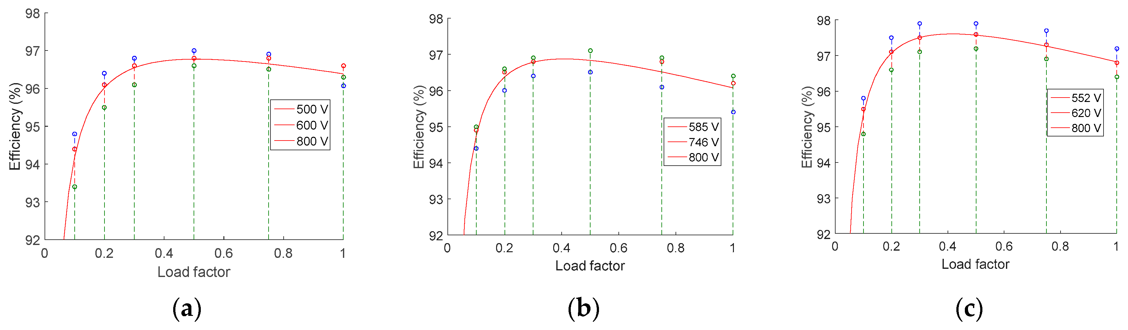
Figure 4 and Figure 5 show the efficiency curves that are computed by the unidimensional models Jantsch and Dupont when they are applied to the inverters under study. The CEC data around the fitted curve have been highlighted. As expected, with both models the predicted values cannot be accurate in all the range of the DC voltage.

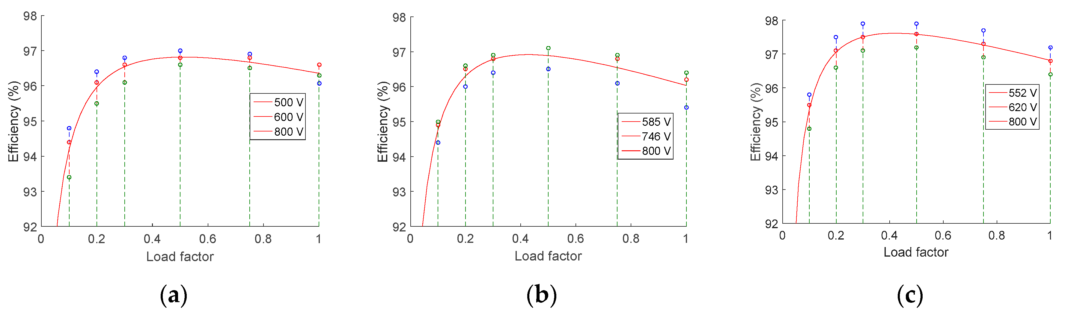
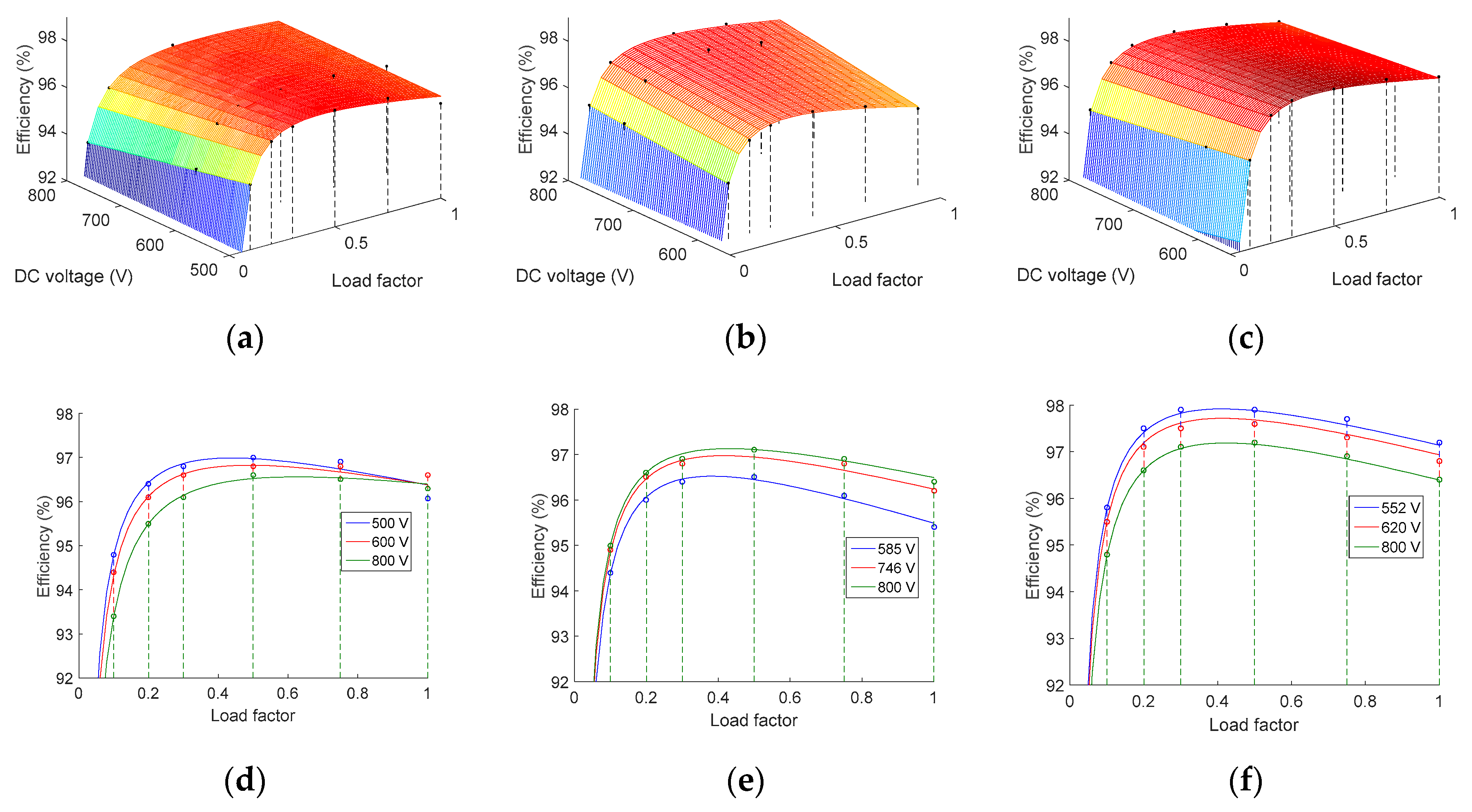
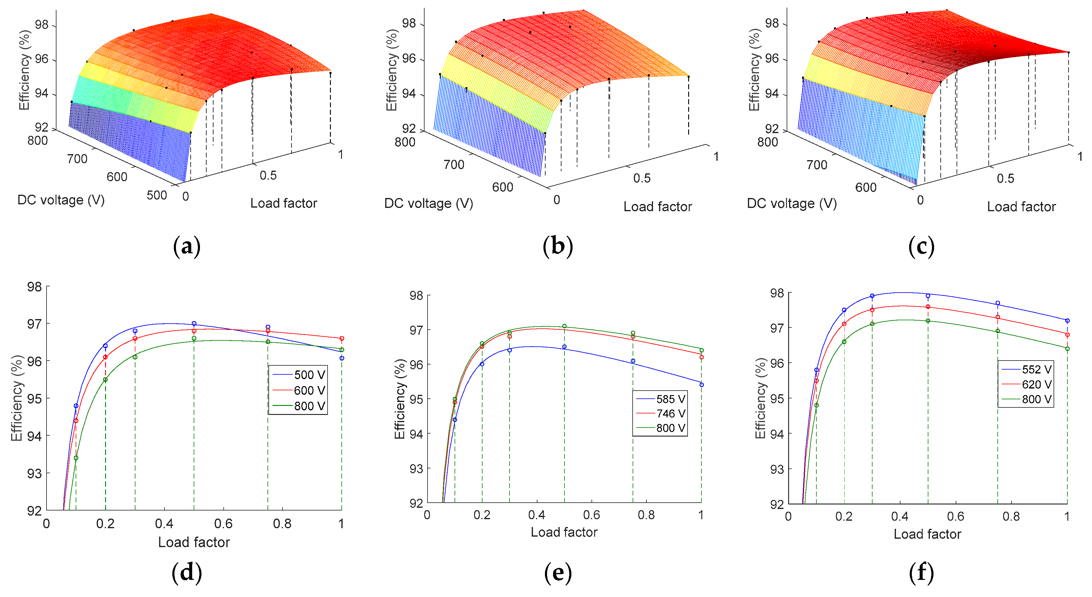
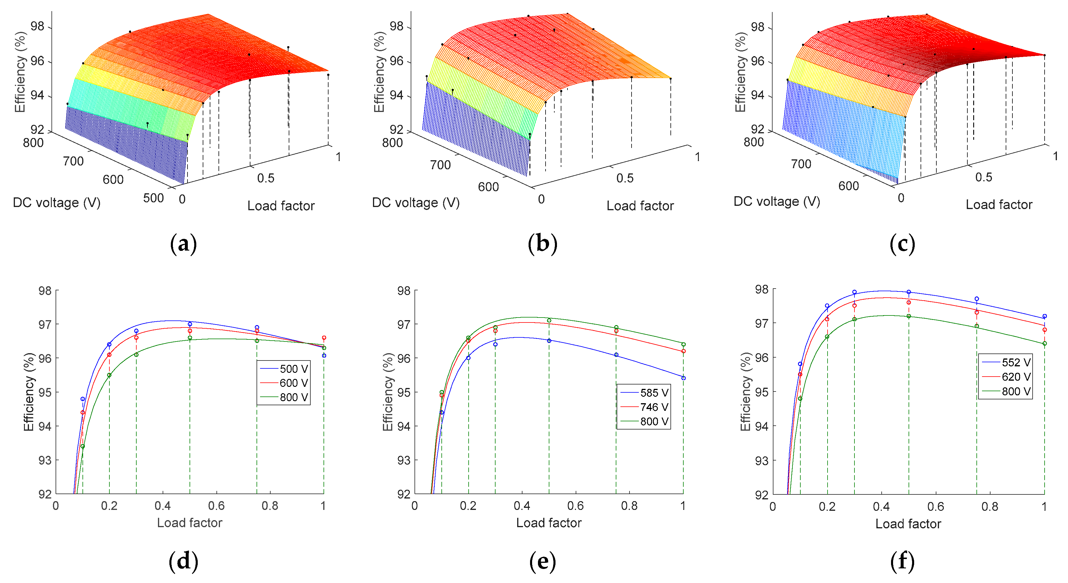
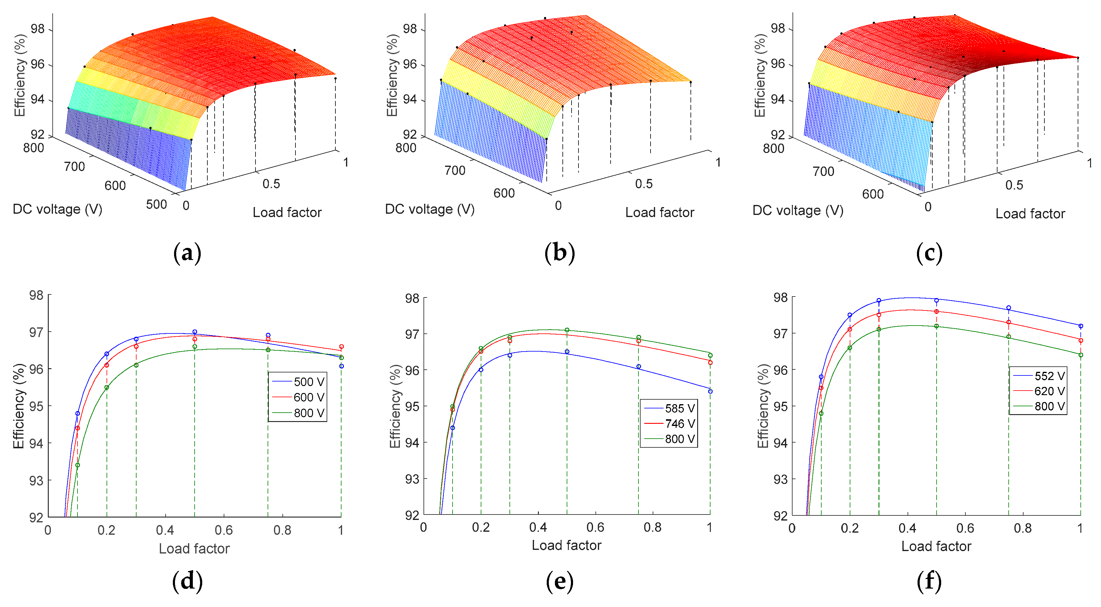
Figure 6a–c show the efficiency surfaces of the inverters, which have been computed by means of the Rampinelli model in the whole range of MPPT voltages. Figure 6d–f detail these results only for the three values of the DC voltage given by CEC. In Figure 7, Figure 8 and Figure 9, the same results are depicted, obtained in the same conditions, but in these cases by means of Rampinelli nonlinear model, Sandia model, and Driesse model, respectively. As expected, the results obtained by using bidimensional models significantly improve compared to the ones achieved by means of the unidimensional ones. Regarding the dependence of the efficiency curves with v_in, note that for the inverter #2 (Power-One ULTRA-750-TL-OUTD-4-US) there are no significant differences between the results offered by the four evaluated bidimensional models. The reason for that is the strong linear dependence with the DC voltage that the efficiency curves of this inverter present. In contrast, in the case of the other two inverters under study, the dependence of the efficiency curves with the DC voltage is not linear and, therefore, the results achieved by means of Rampinelli nonlinear and the Driesse models fit better with the actual CEC data than the Rampinelli and the Sandia models.

In summary, it may be concluded that the Rampinelli nonlinear and the Driesse models are the best approaches to predict the performance of photovoltaic inverters in terms of efficiency, independent of the relationship between efficiency and MPP voltage of the inverter.

5.2. Evaluation of the Proposed Efficiency-Oriented (EO) Algorithm

The algorithm for the activation/deactivation of the power modules that were described in Section 4 is applied in this section to a central inverter with a nominal power of 3 MW. The algorithm has been tested considering two significant profiles of photovoltaic generation, in sunny and cloudy conditions.

Table 11. Number of modules to achieve 3 MW with the inverters under study.

Inverter	Company	Nominal Power	Number of Modules
EQX0250UV480TN	Perfect Galaxy International Ltd.	250 kW	12
ULTRA-750-TL-OUTD-4-US	Power-One	750 kW	4
FS0900CU	Power Electronics	1 MW	3

shows the number of units that are needed to achieve the nominal power with the commercial inverters under study.

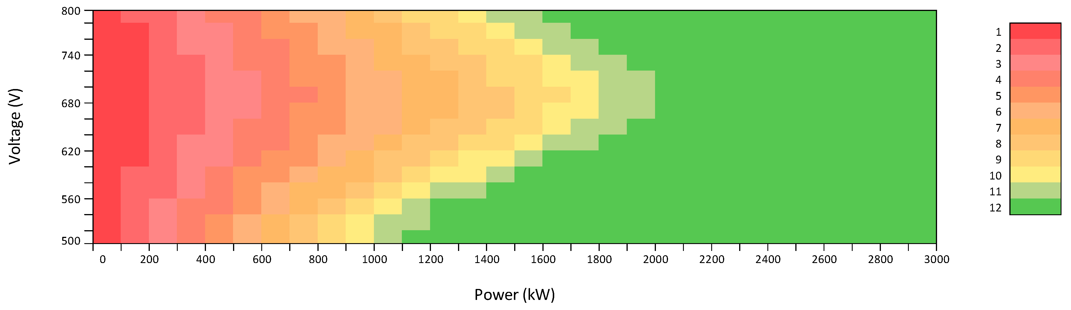
As explained in Section 3, for a certain set of values of both the load factor and the MPP voltage, the algorithm calculates the optimal number of connected modules to maximize the efficiency of the whole system. To illustrate by means of an example how the algorithm works, Figure 10 shows the optimal number of modules on stream that are calculated by the proposed EO algorithm for a 3 MW central inverter composed by twelve modules of Perfect Galaxy International Ltd. EQX0250UV480TN. The figure depicts the number of inverters in operation that maximizes the efficiency in the whole range of MPP voltages and power.

The proposed algorithm has been implemented in the TMS320F28379D to evaluate the needed computing resources (execution time and memory). To achieve this, a central inverter composed of twelve modules of the Perfect Galaxy International Ltd. EQX0250UV480TN has been considered. Two options for implementing the algorithm have been evaluated. In the first one, the operation map that Figure 10 shows has been programmed by means of a lookup (LU) table. With this approach, the algorithm equations are not solved in real time, so the execution time of the algorithm is expected to be low. In return, the memory requirements increase due to the need of storing in the DSP all the points of the operation map. The second option to implement the algorithm is directly programming the equations in the DSP and solve them in real time. In this case, lower memory requirements and larger execution time are expected than in the case of using a lookup table.

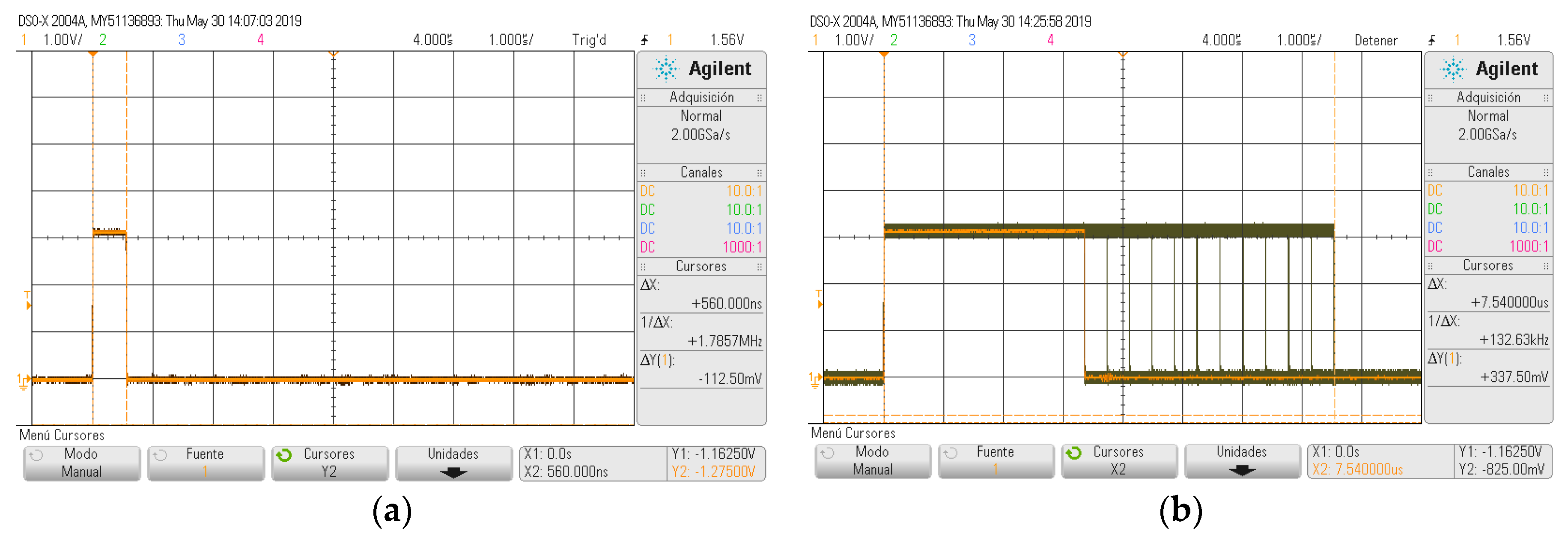
Figure 11a shows the execution time for option #1. In the case under study (12 modules in parallel), the chosen lookup table has a size 15 × 60 (15 input voltages and 60 power levels), needing 1800 bytes of data memory and 47 words of program memory. With this implementation, the algorithm use and its execution time is 540 ns. Note that the memory resources could vary depending on the resolution of the LU table.

Figure 11b shows the measured execution time when the equations of the algorithm are solved in real time. Note that, in this case, the execution time depends on the number of iterations performed by the algorithm, which are related to the number of modules that compose the central inverter and also on the power generated by the PV field. In the case under study, the execution time at low power is 7.54 µs and at high power is reduced to approximately 3.5 µs. The reason for this difference is that at low power, the efficiency must be calculated considering 1 to n inverters on stream. When the power generation increases, the execution time decreases since the algorithm does not calculate the efficiency when the power managed by each module is greater than its nominal power. In other words, the iteration of the loop is not executed when c_mod-i > 1, as it can be seen in Figure 2. The program memory used in this case is 37 words and the use of data memory is negligible.

Table 12. Execution time and memory resources.

Implementation	Data Memory	Program Memory	Execution Time
Option #1	1800 bytes	47 words	540 ns
Option #2	-	37 words	3.5–7.4 µs

summarizes the measured execution times as well as the memory resources for both implementations. The results confirm the expectations about execution time and memory requirements of both kind of implementations, so the choice for a certain application would depend on the need for reducing the implementation time or memory.

5.2.1. Global Efficiency in the Whole Range of Operation of the PV Farm

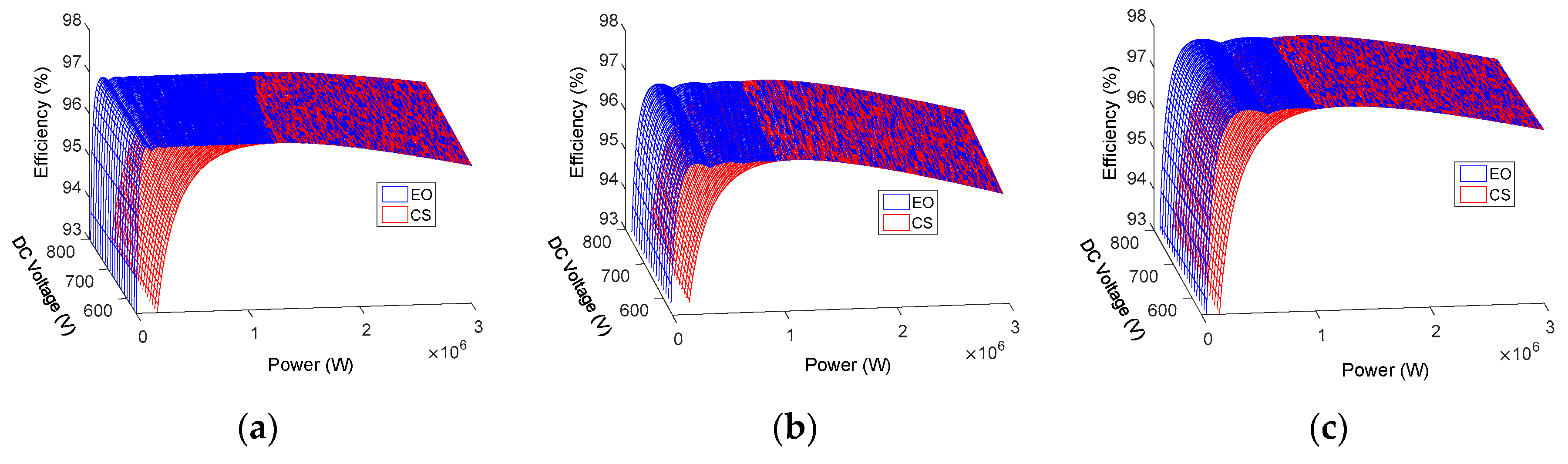
Figure 12 depicts the efficiency surfaces obtained by applying the conventional average current-sharing control method (CS) and the efficiency-oriented (EO) method algorithm of activation/deactivation to the 3 MW central inverter described before.

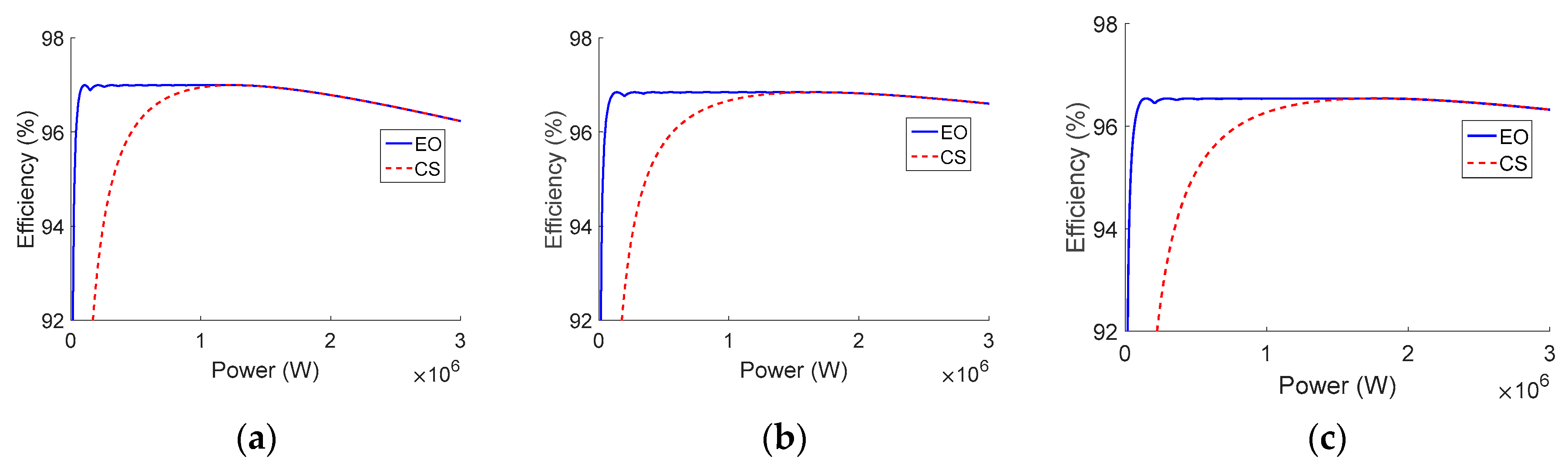
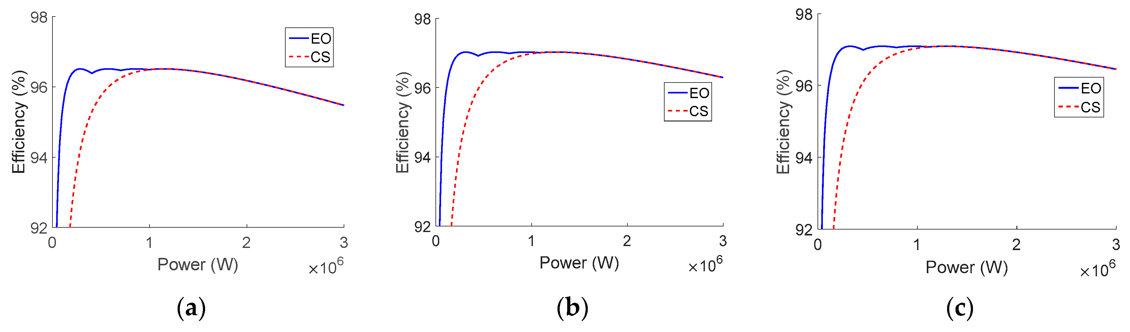
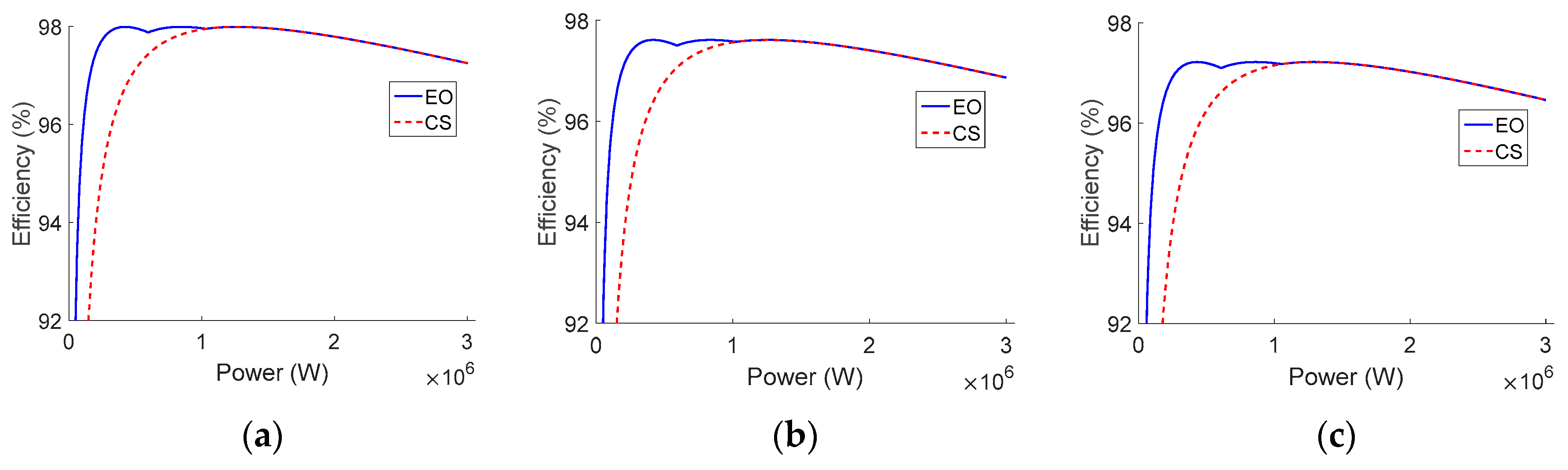
Figure 13a–c depict the detail at 500, 600, and 800 V of the efficiency obtained by both methods applied to the central inverter composed of twelve modules of Perfect Galaxy International Ltd. EQX0250UV480TN. Similarly, Figure 14 and Figure 15 show the results considering the central inverters composed of four modules of Power-One ULTRA-750-TL-OUTD-4-US and three modules of Power Electronics FS0900CU, respectively.

These results show that the efficiency-oriented method achieves the best global efficiency in the whole power range independently of the kind of commercial inverter used to build up the central inverter.

5.2.2. Study for a Typical Daily Power Profile

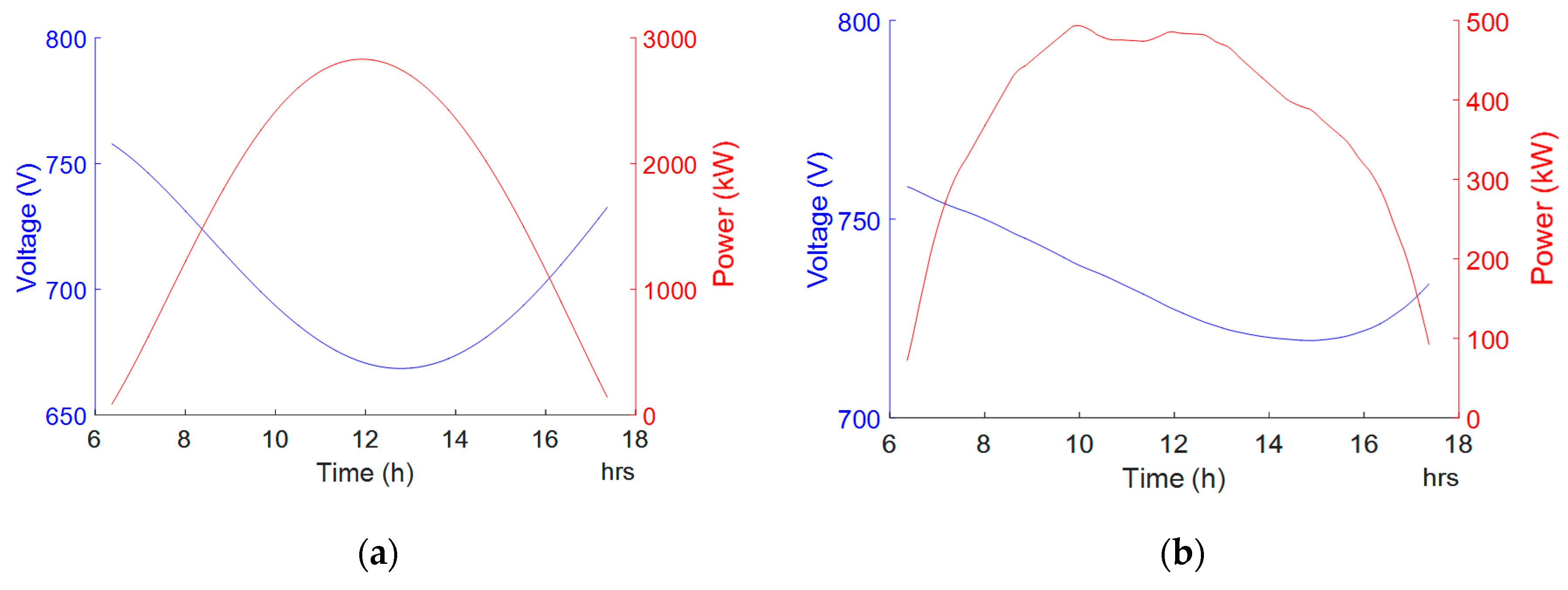
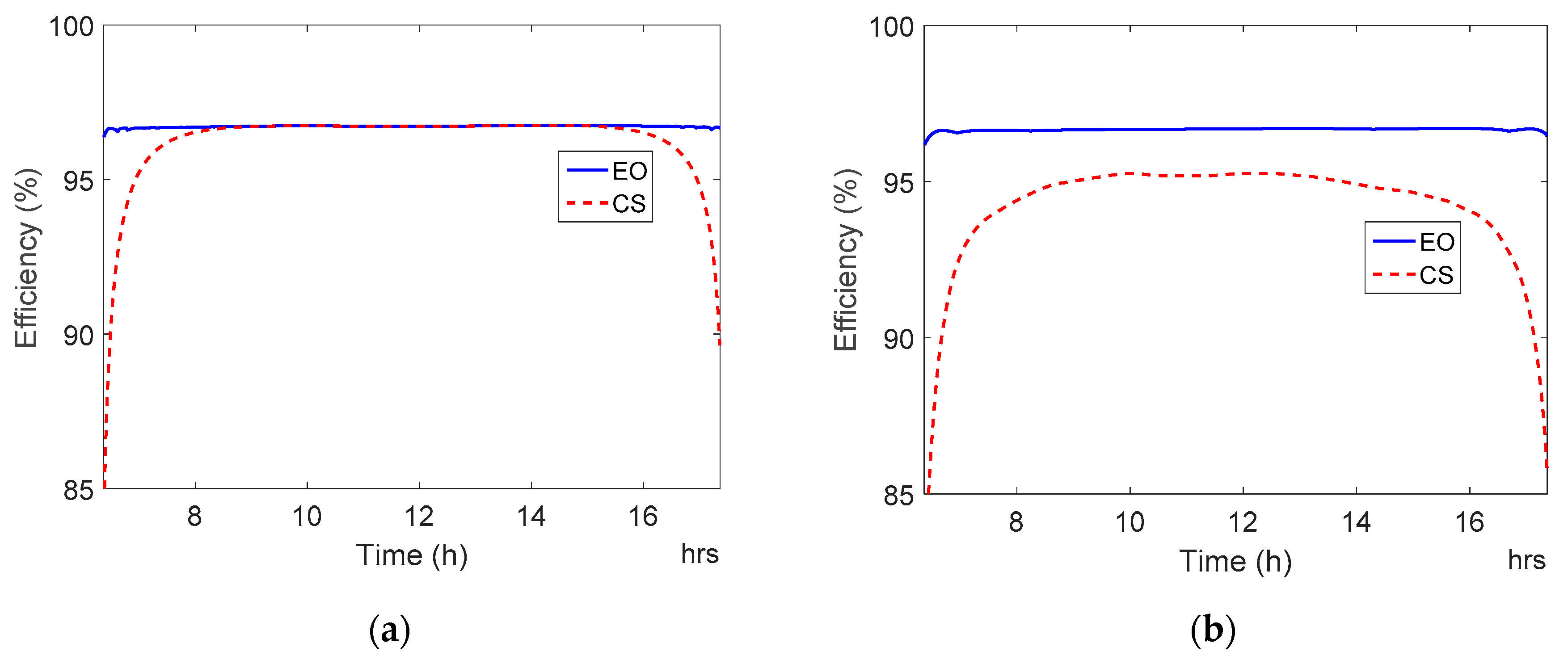
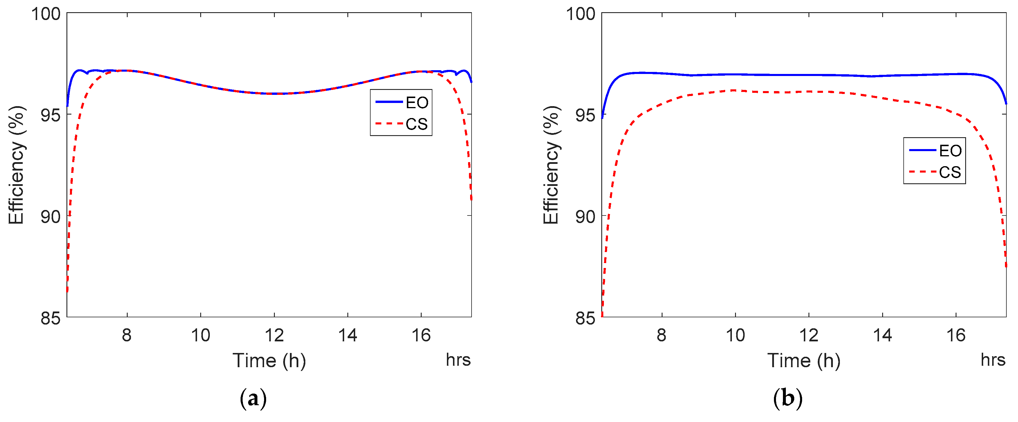
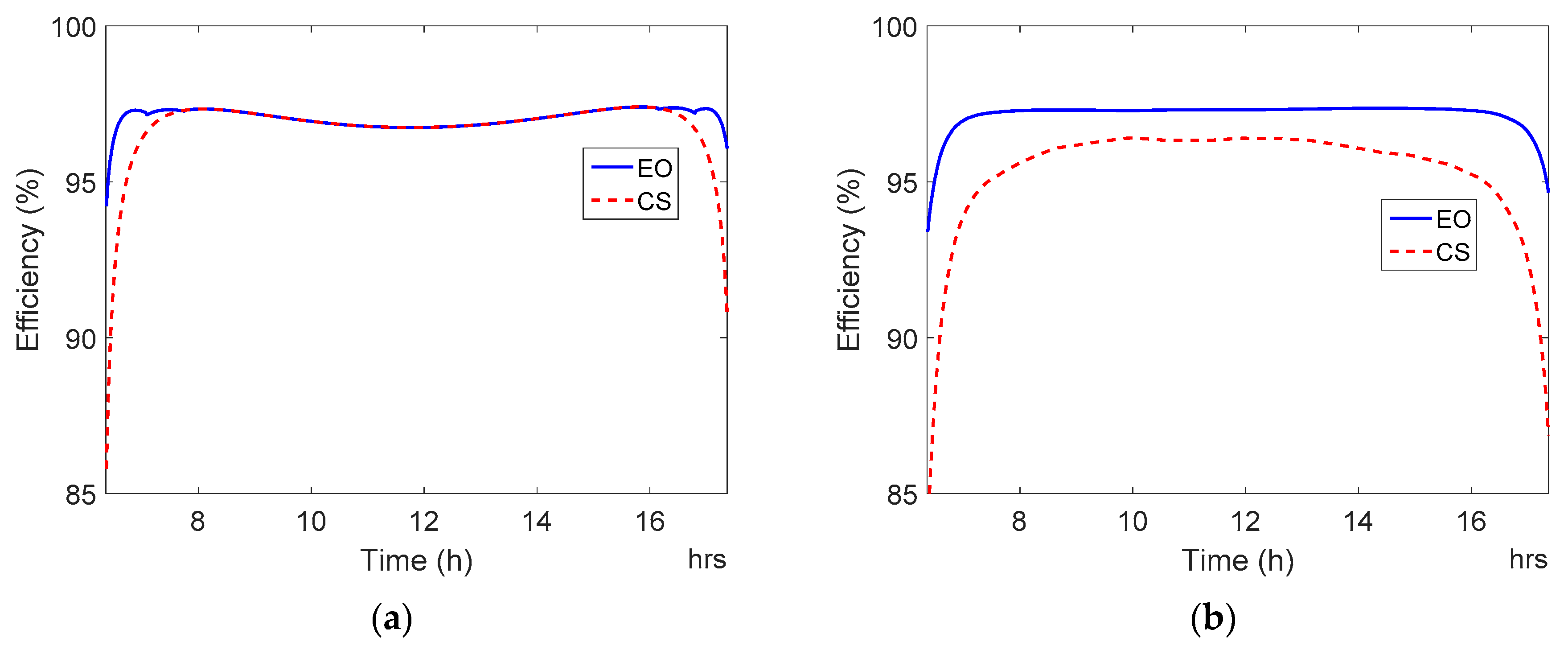
To evaluate the performance of the proposed EO method in realistic conditions, generation profiles in different scenarios have been considered. Figure 16a shows a typical sunny day generation profile while Figure 16b shows a cloudy day generation profile. In the graphics, both the generated power and the DC voltage vary simultaneously.

Figure 17a, Figure 18a and Figure 19a show the efficiency of the evaluated 3 MW central inverter by considering a typical generation profile on a sunny day. Figure 17b, Figure 18b and Figure 19b shows the efficiency of the inverters by considering a typical generation profile on a cloudy day. It can be noticed that, for the central inverters composed by different commercial inverters, the performance of the proposed EO method is clearly better than the efficiency applying the current-sharing method, CS, considering both the sunny and the cloudy day.

6. Conclusions

A control technique to activate/deactivate the power modules of high-power central inverters has been proposed in this paper. The proposed method maintains the advantages of conventional current sharing methods that are usually used to manage the parallel connection of power inverters, as the low need for computational resources, easy implementation, and capability to operate in real time conditions.

The proposed efficiency oriented method is based on a functional model of PV inverters that predicts the efficiency of the system starting from the measurements of the processed power and the MPPT voltage and takes decisions about the number of inverters that should be on stream to improve the global efficiency of the whole central inverter.

A comparative study of several kinds of models to calculate the efficiency of PV inverters has been carried out. The models have been tested by using data of commercial inverters from the “Grid Support Inverters List” published by the California Energy Commission. Unidimensional and bidimensional models have been evaluated, showing that bidimensional and nonlinear models fit much better with the available data. It can then be concluded that bidimensional and nonlinear models are the best choice to be implemented in the proposed EO method.

Regarding the implementation of the proposed algorithm, two options have been evaluated, showing that the execution time can be significantly reduced by implementing the operation map in the whole power and voltage ranges by means of a lookup table. On the contrary, the memory requirements are much lower if the equations of the algorithm are implemented and solved in real time. Therefore, it can be concluded that the choice for a certain application would depend on which factor is preferred to be reduced.

The proposed algorithm of activation/deactivation of the power modules has been applied to a PV field with a nominal power of 3 MW. The inverter’s efficiency achieved by the proposed EO method has been compared to the one with the current sharing technique in the whole range of operation of the PV farm. Moreover, the algorithm has been tested considering two significant profiles of photovoltaic generation, in sunny and cloudy conditions. At the beginning and the end of the day in both profiles, when the PV generation is low, the global efficiency is clearly improved with regard to the conventional current sharing method. Moreover, in cloudy conditions, the improvement is significant during all day.

References

- Wu, H.; Locment, F.; Sechilariu, M. Experimental Implementation of a Flexible PV Power Control Mechanism in a DC Microgrid. Energies 2019, 12, 1233. [Google Scholar] [CrossRef]
- Strzalka, A.; Alam, N.; Duminil, E.; Coors, V.; Eicker, U. Large scale integration of photovoltaics in cities. Appl. Energy 2012, 93, 413–421. [Google Scholar] [CrossRef]
- Zhanga, P.; Li, W.; Li, S.; Wang, Y.; Xiao, W. Reliability assessment of photovoltaic power systems: Review of current status and future perspectives. Appl. Energy 2013, 104, 822–833. [Google Scholar] [CrossRef]
- Kim, Y.S.; Kang, S.-M.; Winston, R. Modeling of a concentrating photovoltaic system for optimum land use. Prog. Photovolt. Res. Appl. 2013, 21, 240–249. [Google Scholar] [CrossRef]
- Müller, B.; Hardt, L.; Armbruster, A.; Kiefer, K.; Reise, C. Yield predictions for photovoltaic power plants: Empirical validation, recent advances and remaining uncertainties. Prog. Photovolt. Res. Appl. 2016, 24, 570–583. [Google Scholar] [CrossRef]
- Borrega, M.; Marroyo, L.; González, R.; Balda, J.; Agorreta, J.L. Modeling and Control of a Master–Slave PV Inverter With N-Paralleled Inverters and Three-Phase Three-Limb Inductors. IEEE Trans. Power Electron. 2013, 28, 2842–2855. [Google Scholar] [CrossRef]
- Araujo, S.V.; Zacharias, P.; Mallwitz, R. Highly Efficient Single-Phase Transformerless Inverters for Grid-Connected Photovoltaic Systems. IEEE Trans. Ind. Electron. 2010, 57, 3118–3128. [Google Scholar] [CrossRef]
- Mohd, A.; Ortjohann, E.; Morton, D.; Omari, O. Review of control techniques for inverters parallel operation. Electr. Power Syst. Res. 2010, 80, 1477–1487. [Google Scholar] [CrossRef]
- Su, J.; Liu, C. A Novel Phase-Shedding Control Scheme for Improved Light Load Efficiency of Multiphase Interleaved DC–DC Converters. IEEE Trans. Power Electron. 2013, 28, 4742–4752. [Google Scholar] [CrossRef]
- Ahn, Y.; Jeon, I.; Roh, J. A Multiphase Buck Converter with a Rotating Phase-Shedding Scheme For Efficient Light-Load Control. IEEE J. Solid-State Circuits 2014, 49, 2673–2683. [Google Scholar] [CrossRef]
- Chen, Y.; Hsu, J.; Ang, Y.; Yang, T. A new phase shedding scheme for improved transient behavior of interleaved Boost PFC converters. In Proceedings of the 2014 IEEE Applied Power Electronics Conference and Exposition—APEC 2014, Fort Worth, TX, USA, 16–20 March 2014; pp. 1916–1919. [Google Scholar]
- Peng, H.; Anderson, D.I.; Hella, M.M. A 100 MHz Two-Phase Four-Segment DC-DC Converter With Light Load Efficiency Enhancement in 0.18/spl mu/m CMOS. IEEE Trans. Circuits Syst. Regul. Pap. 2013, 60, 2213–2224. [Google Scholar] [CrossRef]
- Costabeber, A.; Mattavelli, P.; Saggini, S. Digital Time-Optimal Phase Shedding in Multiphase Buck Converters. IEEE Trans. Power Electron. 2010, 25, 2242–2247. [Google Scholar] [CrossRef]
- Dupont, F.H.; Zaragoza, J.; Rech, C.; Pinheiro, J.R. A new method to improve the total efficiency of parallel converters. In Proceedings of the 2013 Brazilian Power Electronics Conference, Gramado, Brazil, 27–31 October 2013; pp. 210–215. [Google Scholar]
- Huang, W.; Liao, S.; Teng, J.; Hsieh, T.; Lan, B.; Chiang, C. Intelligent control scheme for output efficiency improvement of parallel inverters. In Proceedings of the 2016 IEEE/ACIS 15th International Conference on Computer and Information Science (ICIS), Okayama, Japan, 26–29 June 2016; pp. 1–6. [Google Scholar]
- Effler, S.; Halton, M.; Rinne, K. Efficiency-Based Current Distribution Scheme for Scalable Digital Power Converters. IEEE Trans. Power Electron. 2011, 26, 1261–1269. [Google Scholar] [CrossRef]
- Monteiro, L.; Finelli, I.; Quinan, A.; Macêdo, W.N.; Torres, P.; Pinho, J.T.; Nohme, E.; Marciano, B.; Silva, S.R. Implementation and Validation of Energy Conversion Efficiency Inverter Models for Small PV Systems in the North of Brazil. In Renewable Energy in the Service of Mankind Vol II; Springer: Cham, Switzerland, 2016; pp. 93–102. [Google Scholar]
- Sánchez Reinoso, C.R.; Milon, D.H.; Buitrago, R.H. Simulation of photovoltaic centrals with dynamic shading. Appl. Energy 2013, 103, 278–289. [Google Scholar] [CrossRef]
- Muñoz, J.; Martínez-Moreno, F.; Lorenzo, E. On-site characterisation and energy efficiency of grid-connected PV inverters. Prog. Photovolt. Res. Appl. 2011, 19, 192–201. [Google Scholar] [CrossRef]
- Dupont, F.H.; Zaragoza Bertomeu, J.; Rech, C.; Pinheiro, J.R. A simple control strategy to increase the total efficiency of multi-converter systems. In Proceedings of the Brazilian Power Electronics Conference, Gramado, Brazil, 27–31 October 2013; pp. 284–289. [Google Scholar]
- Baumgartner, F.P. Euro Realo Inverter Efficiency: Dc-Voltage Dependency. In Proceedings of the 20th European Photovoltaic Solar Energy Conference, Barcelona, Spain, 6–10 June 2005. [Google Scholar]
- Davila-Gomez, L.; Colmenar-Santos, A.; Tawfik, M.; Castro-Gil, M. An accurate model for simulating energetic behavior of PV grid connected inverters. Simul. Model. Pract. Theory 2014, 49, 57–72. [Google Scholar] [CrossRef] [Green Version]
- Rampinelli, G.A.; Krenzinger, A.; Romero, F. Mathematical models for efficiency of inverters used in grid connected photovoltaic systems. Renew. Sustain. Energy Rev. 2014, 34, 578–587. [Google Scholar] [CrossRef]
- King, D.L.; Gonzalez, S.; Galbraith, G.M.; Boyson, W.E. Performance Model for Grid-Connected Photovoltaic Inverters; Sandia National Laboratories: Albuquerque, NM, USA, 2007.
- Driesse, A.; Jain, P.; Harrison, S. Beyond the curves: Modeling the electrical efficiency of photovoltaic inverters. In Proceedings of the 2008 33rd IEEE Photovoltaic Specialists Conference, San Diego, CA, USA, 11–16 May 2008; pp. 1–6. [Google Scholar]
- California Energy Commission Grid Support Inverters List. Available online: https://www.gosolarcalifornia.ca.gov (accessed on 14 May 2019).
- Mathai, A.M.; Haubold, H. Fractional and Multivariable Calculus: Model Building and Optimization Problems; Springer: Cham, Switzerland, 2017; ISBN 978-3-319-59993-9. [Google Scholar]
- MathWorks Statistics and Machine Learning Toolbox. Available online: https://www.mathworks.com (accessed on 14 May 2019).
Figure 1.
Topologies of high power central inverters. (a) Centralized inverter composed by a single power stage; (b) centralized inverter composed by n parallel modules.
Figure 2.
Efficiency-oriented algorithm.
Figure 3.
Relationship between the input voltage and the efficiency of the inverters extracted from the CEC Grid Support Inverters List.
Figure 4.
Efficiency curves calculated by means of the Jantsch model. (a) Perfect Galaxy International Ltd. EQX0250UV480TN. (b) Power-One ULTRA-750-TL-OUTD-4-US (c) Power Electronics FS0900CU.
Figure 5.
Efficiency curves calculated by means of the Dupont model. (a) Perfect Galaxy International Ltd. EQX0250UV480TN. (b) Power-One ULTRA-750-TL-OUTD-4-US. (c) Power Electronics FS0900CU.
Figure 6.
Efficiency surfaces and detail of curves for three values of the DC voltage calculated by means of the Rampinelli model. (a,d) Perfect Galaxy International Ltd. EQX0250UV480TN. (b,e) Power-One ULTRA-750-TL-OUTD-4-US. (c,f) Power Electronics FS0900CU.
Figure 7.
Efficiency surfaces and detail of curves for three values of the DC voltage calculated by means of the Rampinelli nonlinear model. (a,d) Perfect Galaxy International Ltd. EQX0250UV480TN. (b,e) Power-One ULTRA-750-TL-OUTD-4-US. (c,f) Power Electronics FS0900CU.
Figure 8.
Efficiency surfaces and detail of curves for three values of the DC voltage calculated by means of the Sandia model. (a,d) Perfect Galaxy International Ltd. EQX0250UV480TN. (b,e) Power-One ULTRA-750-TL-OUTD-4-US. (c,f) Power Electronics FS0900CU.
Figure 9.
Efficiency surfaces and detail of curves for three values of the DC voltage calculated by means of the Driesse model. (a,d) Perfect Galaxy International Ltd. EQX0250UV480TN. (b,e) Power-One ULTRA-750-TL-OUTD-4-US. (c,f) Power Electronics FS0900CU.
Figure 10.
Number of inverters in operation depending on the power generation and the maximum power point tracking (MPPT) voltage.
Figure 11.
Execution time of the algorithm (a) lookup table implementation. (b) equations implemented and solved in real time.
Figure 12.
Efficiency surfaces with average current-sharing control method (CS) and efficiency-oriented method (EO). (a) Perfect Galaxy International Ltd. EQX0250UV480TN. (b) Power-One ULTRA-750-TL-OUTD-4-US. (c) Power Electronics FS0900CU.
Figure 13.
Efficiency of Perfect Galaxy International Ltd. EQX0250UV480TN with average current-sharing control method (CS) and efficiency-oriented method (EO). (a) 500 V. (b) 600 V. (c) 800 V.
Figure 14.
Efficiency of Power-One ULTRA-750-TL-OUTD-4-US with average current-sharing control method (CS) and efficiency-oriented method (EO). (a) 585 V. (b) 746 V. (c) 800 V.
Figure 15.
Efficiency of Power Electronics FS0900CU with average current-sharing control method (CS) and efficiency-oriented method (EO). (a) 552 V. (b) 620 V. (c) 800 V.
Figure 16.
Daily power generation and MPPT voltage curves. (a) Sunny day. (b) Cloudy day.
Figure 17.
Daily efficiency curves of Perfect Galaxy International Ltd. EQX0250UV480TN with average current-sharing control method (CS) and efficiency-oriented method (EO). (a) Sunny day. (b) Cloudy day.
Figure 18.
Daily efficiency curves of Power-One ULTRA-750-TL-OUTD-4-US with average current-sharing control method (CS) and efficiency-oriented method (EO). (a) Sunny day. (b) Cloudy day.
Figure 19.
Daily efficiency curves of Power Electronics FS0900CU with average current-sharing control method (CS) and efficiency-oriented method (EO). (a) Sunny day. (b) Cloudy day.