Aggregation of Type-4 Large Wind Farms Based on Admittance Model Order Reduction

Abstract

This paper presents an aggregation technique based on the resolution of a multi-objective optimization problem applied to the admittance model of a wind power plant (WPP). The purpose of the presented aggregation technique is to reduce the order of the wind power plant model in order to accelerate WPP simulation while keeping a very similar control performance for both the simplified and the detailed models. The proposed aggregation technique, based on the admittance model order reduction, ensures the same DC gain, the same gain at the operating band frequency, and the same resonant peak frequency as the detailed admittance model. The proposed aggregation method is validated considering three 400-MW grid-forming Type-4 WPPs connected to a diode rectifier HVDC link. The proposed aggregation technique is compared to two existing aggregation techniques, both in terms of frequency and time response. The detailed and aggregated models have been tested using PSCAD-EMTsimulations, with the proposed aggregated model leading to a 350-fold reduction of the simulation time with respect to the detailed model. Moreover, for the considered scenario, the proposed aggregation technique offers simulation errors that are, at least, three-times smaller than previously-published aggregation techniques.

1. Introduction

Large off-shore wind power plants (WPPs) with more than one hundred wind turbine generators (WTG) are currently operational or in the planning or approval phases. Simulation studies covering individual WTGs during the design phase are very demanding from the computational point of view. When studying the impact of WPPs in the overall HVDC or HVAC transmission network, very detailed models are not generally required. Therefore, simulation complexity and computing time can be reduced by using aggregated WTG models. However, these aggregated models should provide a faithful representation of the actual WPP dynamics.

This is particularly important if the WPP consists of grid-forming converters, such as when using diode rectifier (DR)-based HVDC stations for the connection of the offshore WPP. The use of DR HVDC stations can significantly reduce capital expenditure (CAPEX) and operational expenditure (OPEX) by increasing the efficiency and robustness of the overall system [1,2,3,4,5,6]. However, a large number of case studies is required in order to verify the correct integration of DR-connected WPPs.

Therefore, this paper is focused on the procedure to obtain an aggregated WTG model for large Type-4 WPPs that allows the verification of grid-forming WTG controllers for DR HVDC station connection. The presented aggregation technique aims at reducing the computational requirements of such a verification, while achieving better simulation accuracy than current state-of-the-art aggregation techniques.

A large amount of literature has been developed on aggregation techniques for different applications [7,8]. For example, the work in [9] presented an aggregation technique based on power losses, while [10] presented an aggregation technique for grid disturbances studies. The work in [11] included a method for Type-3 and Type-1 WTG aggregation suitable for large power systems simulation. In this case, the WPP grid was aggregated using a short-circuit impedance method. In [12], an aggregated method based on voltage drop assumptions was performed as the most appropriate aggregation method for stability assessment studies. On the other hand, in [13], an aggregation method was proposed in order to represent the whole power system seen from the WTG AC terminals. Finally, an improvement on the aggregation method based on power losses for off-shore WPP with a diode-based HVDC link was proposed in [14].

However, none of the previous methods were based on a model order reduction of the total WPP admittance model. The proposed model order reduction leads to better matching between the dynamic behavior of the aggregated and full WPP models, as the aggregated system keeps the original DC admittance, fundamental frequency admittance, and first resonance peak characteristics of the original system.

The paper is organized as follows. The second section shows the procedure to obtain the full admittance model of a typical WPP, consisting of a number of radially-connected WTG strings, as this is the typical topology used in WPPs. Other WPP topologies (i.e., with different degrees of meshing) can also be aggregated with the proposed method, by suitable modification of the analytical admittance calculation. The third section explains how to apply the proposed aggregation technique. The fourth section describes the system that is used in the fifth section to compare the proposed aggregation technique with other existing aggregation techniques found in the literature. The sixth section compares the aggregated and detailed model of a WPP using PSCADsimulations, considering three different cases. The last section includes the discussion of the proposed aggregation technique compared with other existing aggregation algorithms.

2. Full-Order Admittance System Modeling

The proposed model aggregation technique was based on the resolution of a multi-objective optimization problem applied to a full-WPP admittance model. This section includes the analytical development of the WPP admittance model. The inputs to the model were the individual WTG voltages, and its output was the WPP current at the point of common coupling (PCC).

Each considered WPP consisted of n radial-connected strings, with each string consisting of $m_i$ cascaded connected WTGs. This topology corresponds to the great majority of existing WPPs, as ring-connected strings are always exploited radially. In any case, it is very easy to modify the proposed analytical model to calculate the overall grid-admittance of other WPP topologies.

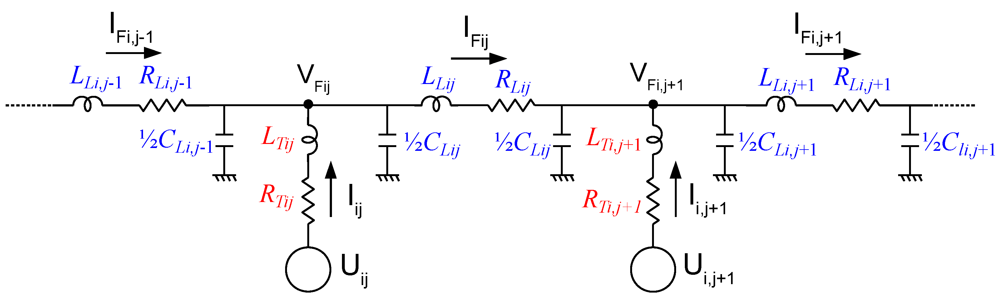
Figure 1 shows the WTG-j ($j=1,2,\dots ,m_i$) in the string-i ($i=1,2,\dots ,n$) of the WPP. $U_{ij}$ is the WTG grid-side converter, and ($L_{Tij}$ and $R_{Tij}$) represents the WTG transformer. Several alternatives have been considered to model the array cables, e.g., [15] added parallel L-R branches to a PI-model in order to represent the frequency-dependent impedance of the cable. This model has been used in [16,17] to obtain a state-space model and reduce the order of the cable model. Additionally, a frequency-dependent PI model of a three-core submarine cable was studied in [18].

In the presented case study, PI-sections will be used to represent the cable dynamics ($C_{Lij}$, $L_{Lij}$, and $R_{Lij}$), since the cable length between WTGs was less than 3 km with its resonant peak at frequencies higher than 1000 Hz. The use of PI-models offers a good trade-off between complexity and accuracy.

2.1. String Admittance Model

The dynamics of the WTG-j ($j=1,2,\dots ,m_i$) and cable shown in Figure 1 can be written as:

$$U_{ij}=R_{Tij}·I_{ij}+L_{Tij}·\frac{d{I}_{ij}}{dt}+V_{Fij}$$

(1)

$$I_{Fi,j-1}+I_{ij}-I_{Fij}=\left(\frac{C_{Li,j-1}}{2}+\frac{C_{Lij}}{2}\right)·\frac{d{V}_{Fij}}{dt}$$

(2)

$$V_{Fij}=R_{Lij}·I_{Fij}+L_{Lij}·\frac{d{I}_{Fij}}{dt}+V_{Fi,j+1}$$

(3)

where $I_{ij}$ is the current from WTG-j, $V_{Fij}$ is the voltage at the secondary side of the transformer, and $I_{Fij}$ is the current through the cable. Note that for $j=1$ (leftmost WTG), the current $I_{Fi,j-1}$ did not exist, and for $j=m_i$ (rightmost WTG), the voltage $V_{Fi,j+1}$ was the PCC voltage ($V_F$), which was considered a disturbance.

From Equations (1)–(3), the state-space admittance model of string-i ($i=1,2,\dots ,n$) can be calculated as:

$${\dot{x}}_{st,i}=A_{st,i}·x_{st,i}+B_{st,i}·u_{st,i}+W_{st,i}·V_F$$

(4)

$$y_{st,i}=C_{st,i}·x_{st,i}$$

(5)

where the state vector $x_{st,i}$ and the input vector $u_{st,i}$ are:

$$x_{st,i}=\left[\begin{array}{cccccccccc}{I}_{i1}& V_{Fi1}& I_{Fi1}& I_{i2}& V_{Fi2}& I_{Fi2}& \cdots & I_{i,m_i}& V_{Fi,m_i}& I_{Fi,m_i}\end{array}\right],u_{st,i}={\left[\begin{array}{cccc}{U}_{i1}& U_{i2}& \cdots & U_{i,m_i}\end{array}\right]}^T$$

Matrices $A_{st,i}$, $B_{st,i}$, and $C_{st,i}$ are the state, input, and output matrices, respectively:

$$A_{st,i}=\left[\begin{array}{cccccccccc}\frac{-R_{Ti1}}{L_{Ti1}}& \frac{-1}{L_{Ti1}}& 0& 0& 0& 0& & 0& 0& 0\\ \frac{2}{C_{Li1}}& 0& \frac{-2}{C_{Li1}}& 0& 0& 0& & 0& 0& 0\\ 0& \frac{1}{L_{Li1}}& \frac{-R_{Li1}}{L_{Li1}}& 0& \frac{-1}{L_{Li1}}& 0& & 0& 0& 0\\ 0& 0& 0& \frac{-R_{Ti2}}{L_{Ti2}}& \frac{-1}{L_{Ti2}}& 0& & 0& 0& 0\\ 0& 0& \frac{2}{C_{Li1}+C_{Li2}}& \frac{2}{C_{Li1}+C_{Li2}}& 0& \frac{-2}{C_{Li1}+C_{Li2}}& & 0& 0& 0\\ 0& 0& 0& 0& \frac{1}{L_{Li2}}& \frac{-R_{Li2}}{L_{Li2}}& & 0& 0& 0\\ & & & & & & \ddots & & & \\ 0& 0& 0& 0& 0& 0& & \frac{-R_{Ti,m_i}}{L_{Ti,m_i}}& \frac{-1}{L_{Ti,m_i}}& 0\\ 0& 0& 0& 0& 0& 0& & \frac{2}{C_{Li,m_i-1}+C_{Li,m_i}}& 0& \frac{-2}{C_{Li,m_i-1}+C_{Li,m_i}}\\ 0& 0& 0& 0& 0& 0& & 0& \frac{1}{L_{Li,m_i}}& \frac{-R_{Li,m_i}}{L_{Li,m_i}}\end{array}\right]$$

$$B_{st,i}=\left[\begin{array}{cccc}\frac{1}{L_{Ti1}}& 0& & 0\\ 0& 0& & 0\\ 0& 0& & 0\\ 0& \frac{1}{L_{Ti2}}& & 0\\ 0& 0& & 0\\ 0& 0& & 0\\ & & \ddots & \\ 0& 0& & \frac{1}{L_{Ti,m_i}}\\ 0& 0& & 0\\ 0& 0& & 0\end{array}\right],C_{st,i}=\left[\begin{array}{cccccccccc}0& 0& 0& 0& 0& 0& \cdots & 0& 0& 1\end{array}\right]$$

and:

$$W_{st,i}={\left[\begin{array}{cccccccccc}0& 0& 0& 0& 0& 0& \cdots & 0& 0& \frac{-1}{L_{Li,m_i}}\end{array}\right]}^T$$

2.2. Overall Admittance Model

The admittance model of the complete WPP was obtained by the radial connection of the n strings to the PCC (represented by voltage $V_F$). The state space dynamics of the overall system are:

$${\dot{x}}_o=A_o·x_o+B_o·u_o+W_o·V_F$$

(6)

$$y_o=C_o·x_o$$

(7)

where $A_o$, $B_o$, and $C_o$ are the state, input, and output of the overall system obtained by combining the string state space equations:

$$A_o=\left[\begin{array}{cccc}{A}_{st1}& 0& & 0\\ 0& A_{st2}& & 0\\ & & \ddots & \\ 0& 0& & A_{st,n}\end{array}\right],B_o=\left[\begin{array}{cccc}{B}_{st1}& 0& & 0\\ 0& B_{st2}& & 0\\ & & \ddots & \\ 0& 0& & B_{st,n}\end{array}\right]$$

$$C_o=\left[\begin{array}{cccc}{C}_{st1}& C_{st2}& \dots & C_{st,n}\end{array}\right]$$

and:

$$W_o={\left[\begin{array}{cccc}{W}_{st1}& W_{st2}& \dots & W_{st,n}\end{array}\right]}^T$$

3. Aggregation Technique

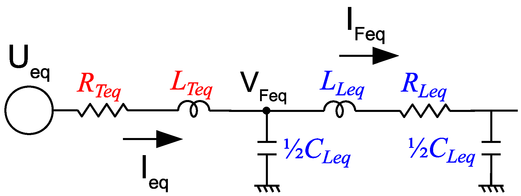
The structure of the aggregated equivalent WPP is shown in Figure 2. At this point, the aggregation technique based on multi-objective optimization was carried out by following these steps:

• Input reduction.
• Multi-objective optimization problem statement.
• Multi-objective optimization problem solution.

3.1. Input Reduction

The proposed admittance model had a total of n voltage inputs that should be reduced to a single voltage input. Using the admittance model of the overall system, the superposition principle can be applied in order to obtain a single-input single-output model. The equivalent single-input voltage source was obtained by introducing the vector $\sigma$ in Equations (6) and (7), leading to Equations (8) and (9):

$$\dot{x}=A·x+B·\sigma ·u$$

(8)

$$y=C·x+D·\sigma ·u$$

(9)

$\sigma$ is a vector with values of one for connected WTGs or zero for disconnected WTG:

$$\sigma ={\left({\sigma }_{1,1},{\sigma }_{1,2},\cdots ,{\sigma }_{i,j},\cdots ,{\sigma }_{n,m_i}\right)}^T$$

The obtained SISO system had a single equivalent voltage input (u) and the WPP PCC current as an output ($I_F=I_{F1,m_1}+I_{F2,m_2}+\dots +I_{Fn,m_n}$) and had a total of $3·n$ states, with n equal to the number of WTGs in the WPP.

3.2. Multi-Objective Optimization Problem Statement

The target aggregated model is shown in Figure 2, with dynamics:

$${\dot{x}}_{eq}=A_{eq}·x_{eq}+B_{eq}·u_{eq}$$

(10)

$$y_{eq}=C_{eq}·x_{eq}+D_{eq}·u_{eq}$$

(11)

where the inputs of the aggregated WTG model $u_{eq}$ were the aggregated voltage source ($U_{eq}$) and the voltage at the point of common coupling ($V_F$). The model output was the WPP current ($I_{Feq}$), and the state variables were $I_{eq}$, $V_{Feq}$, and $I_{Feq}$, as shown in Figure 2.

Matrices $A_{eq}$, $B_{eq}$, $C_{eq}$, and $D_{eq}$ are given below:

$$\begin{array}{cc}{A}_{eq}=\left(\begin{array}{ccc}-\frac{R_{Teq}}{L_{Teq}}& \frac{-1}{L_{Teq}}& 0\\ \frac{1}{\frac{C_{Leq}}{2}}& 0& \frac{-1}{\frac{C_{Leq}}{2}}\\ 0& \frac{1}{L_{Leq}}& -\frac{R_{Leq}}{L_{Leq}}\end{array}\right)& B_{eq}=\left(\begin{array}{cc}\frac{1}{L_{Teq}}& 0\\ 0& 0\\ 0& -\frac{1}{L_{Leq}}\end{array}\right)\end{array}$$

$$\begin{array}{cc}{C}_{eq}=\left(\begin{array}{ccc}0& 0& 1\end{array}\right)& D_{eq}=\left(\begin{array}{cc}0& 0\end{array}\right)\end{array}$$

The reduced order model in Equations (10) and (11) had five parameters to be identified ($L_{Teq}$, $R_{Teq}$, $L_{Leq}$, $R_{Leq}$, and $C_{Leq}$). In order to formulate the multi-optimization problem properly, the following considerations were made:

• The aggregated capacitance $C_{Leq}$ was considered as the sum of the total shunt capacitance in the WPP grid [9].
• The factor $X_T/R_T$ of the WTG transformer shall be maintained in the aggregated transformer ($X_{Ti}/R_{Ti}=X_{Teq}/R_{Teq}$).

At this point, three objectives are proposed to identify the remaining three parameters for the aggregated model, namely:

• Minimize the error between the DC gain of aggregated ($K_{\omega =0}$ Hz) and the high order SISO system ($K_{\omega =0}^{*}$ Hz).
• Minimize the error between the gain of the aggregated WTG model at the grid frequency ($K_{\omega ={\omega }_0}$ Hz) and that of the high order SISO system ($K_{\omega ={\omega }_0}^{*}$ Hz).
• Minimize the error between the frequency of the resonant peak (${\omega }_{peak}$) of the aggregated WTG model and the frequency of the first resonant peak of the high order SISO system (${\omega }_{peak}^{*}$).

Finally, we shall consider that the WTG model parameters to identify always shall be positive and within a defined range ($R_{Teq,min}<R_{Teq}<R_{Teq,max}$, $R_{Leq,min}<R_{Leq}<R_{Leq,max}$, and $L_{Leq,min}<L_{Leq}<L_{Leq,max}$).

From the assumptions above, the following multi-objective optimization function was defined for the aggregated model:

$$f(R_{Teq},L_{Leq},R_{Leq})=\left(\begin{array}{c}{\omega }_{peak}(R_{Teq},L_{Leq},R_{Leq})\\ K_{\omega =0}(R_{Teq},L_{Leq},R_{Leq})\\ K_{\omega =\omega 0}(R_{Teq},L_{Leq},R_{Leq},{\omega }_0)\end{array}\right)$$

(12)

The goal function ($f^{*}$) was obtained from the system described in Equations (8) and (9). Therefore, the aim of the optimization problem was to minimize the maximum of:

$$W_i(f(R_{Teq},L_{Leq},R_{Leq})-f^{*})$$

(13)

where $W_i$ is a diagonal matrix containing the weights to scale each function of $f(R_{Teq},L_{Leq},R_{Leq})$. Additionally, the minimization problem shall satisfy the constraints:

$$\begin{array}{c}\hfill \left(\begin{array}{c}{R}_{Teq,min}\\ L_{Leq,min}\\ R_{Leq,min}\end{array}\right)<\left(\begin{array}{c}{R}_{Teq}\\ L_{Leq}\\ R_{Leq}\end{array}\right)<\left(\begin{array}{c}{R}_{Teq,max}\\ L_{Leq,max}\\ R_{Leq,max}\end{array}\right)\end{array}$$

The multi-objective optimization problem was solved by the goal attainment method described in [19,20,21,22]. The criteria used to choose the initial parameter and weight estimates is included in Section 5.1.

4. HVDC Diode Rectifier-Connected Wind Power Plant

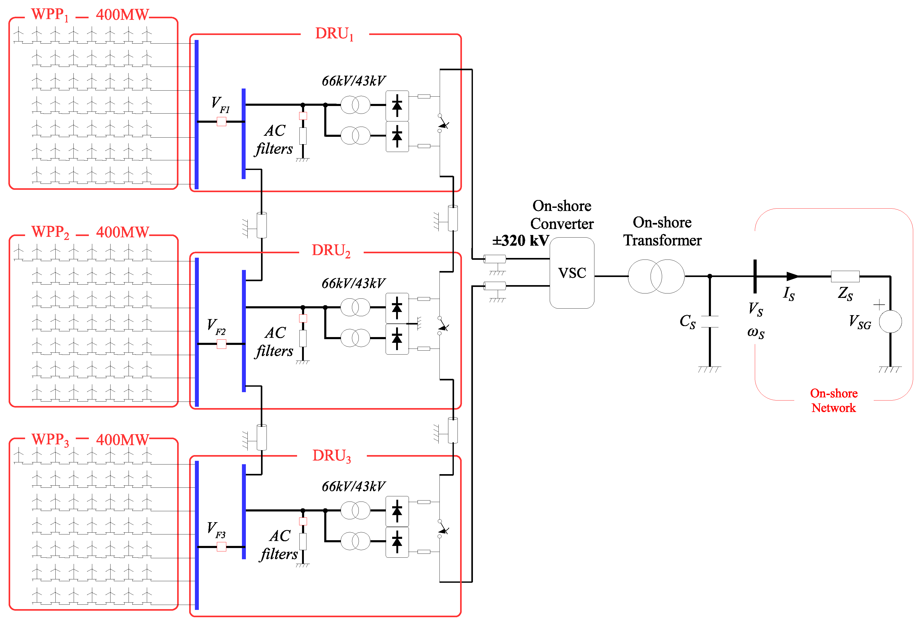
The system under study is shown in Figure 3. It consisted of three 400-MW WPPs connected to the on-shore network through a diode rectifier-based HVDC link [1,14].

Each WPP consisted of 50 Type-4 WTGs rated at 8 MW each. Each WTG generator had a full-scale back-to-back converter, a PWM filter, and a WTG transformer that were connected to the 66-kV off-shore AC grid.

Each one of the three WPPs ($k=1,2,3$) was composed of 50 WTGs, distributed in $n=7$ strings ($i=1,2,\dots n$) with $m_i$ wind turbines per string ($j=1,2,\dots m_i$).

Finally, the rectifier station consisted of three diode rectifier platforms, DC-side series connected. The rectifier stations were connected by means of the HVDC cable to the onshore VSC station, as shown in Figure 3. Each DR station consisted of two 12-pulse DR bridges, together with the corresponding transformers and AC filters [14].

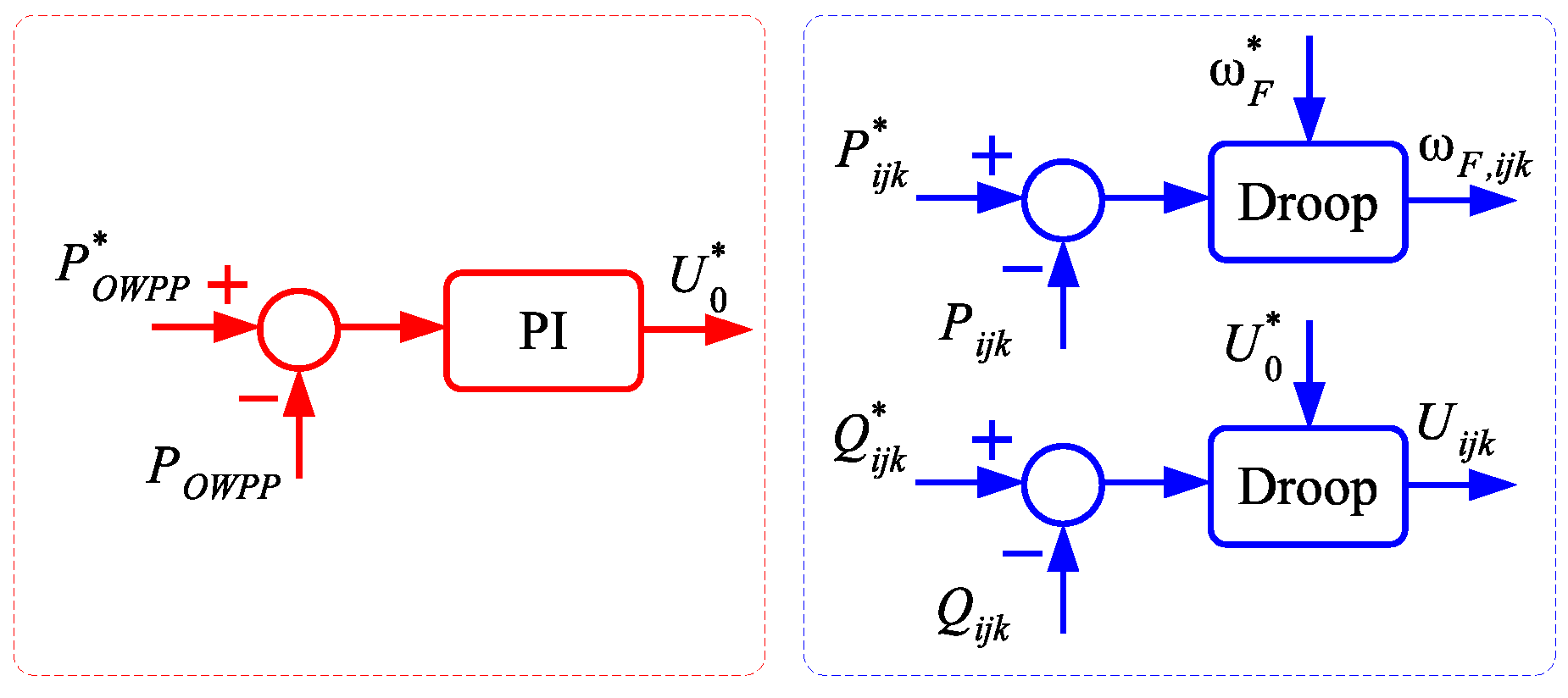
The implemented control is shown in Figure 4. The control consisted of a centralized controller for the total delivered active power $P_{OWPP}$:

$$P_{OWPP}=\sum _{k=1}^3\sum _{i=1}^n\sum _{j=1}^{m_i}{P}_{WTG,ijk}$$

and a distributed controller based on a standard $P/\omega$, $Q/V$ droop controller.

The centralized controller was based on a PI controller operating at a 20-ms sampling time. Using the total optimum power reference from the WTGs ($P_{OWPP}^{*}$) and the actual power being generated by the WPP ($P_{OWPP}$), the controller calculates the reference voltage ($U_0^{*}$) to be used by each individual WTG droop controller. ${\omega }_F^{*}$ is the grid frequency reference. A communication delay of 40 ms was considered for the WPP active power controller.The WPP active power controller had a bandwidth of 4 Hz.

Each WTG implemented a distributed $P/\omega$ and $Q/V$ droop controller. The droop controller calculates the frequency ${\omega }_{Fijk}$ and the voltage $U_{ijk}$ of the WTGs grid side converters (GSC) using the measured and reference active power $P_{ijk}$ and the reactive power $Q_{ijk}$, respectively. Local $P_{ijk}$ and $Q_{ijk}$ measurements were filtered with a 10-rad/s low pass filter. More advanced controllers can also be implemented for P and Q sharing amongst wind turbines [23].

The AC-cable parameters, as well as all those of the system in Figure 3 are listed in the Appendix A.

5. Wind Power Plant Aggregation

This section includes the application of the proposed technique to the described case and its comparison with two well-established aggregation strategies.

5.1. Aggregation Based on Multi-Objective Optimization

The state space admittance model of each one of the wind power plants was obtained following the procedure explained in Section 2, including input reduction with $\sigma$ equal to a vector of ones. The state space model thus obtained was of order 150.

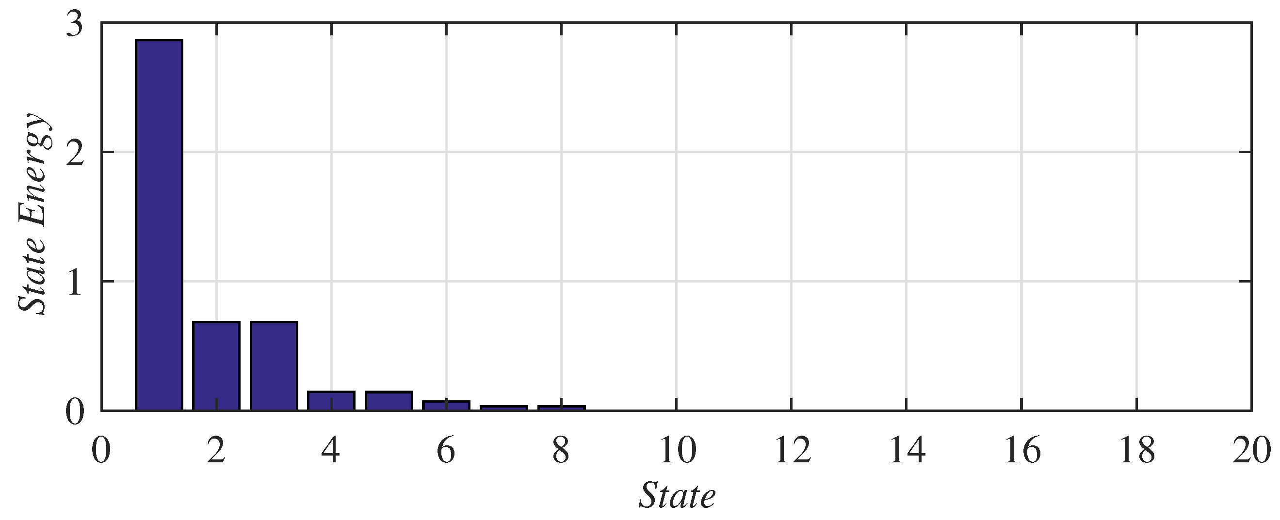
Before carrying out the multi-objective optimization, it is important to ensure that the full system can be reduced to a system with only three states (according to Equations (10) and (11)). To this avail, the contribution of each state has been analyzed obtaining the Hankel singular values of the system. Figure 5 shows that the dynamics of the complete system are mainly dominated by three states; therefore, a third order reduced system can effectively capture most of the dynamic behavior of the full-order system.

To carry out the multi-objective optimization problem, the weights $W_i$ and the restrictions on $R_{Teq}$, $L_{Leq}$, and $R_{Leq}$ need to be defined. To set the weights $W_i$ properly, it is important to notice that the first objective used in the optimization function (12) is related to a frequency, while the other two are related to gains. Therefore, the weight $W_i$ related to the first optimization objective is 1000-times higher than the other two weights. The selected weights $W_i$ are shown in the Appendix A.

The parameters $R_{Teq}$, $L_{Leq}$, and $R_{Leq}$ were restricted to be always positive. Moreover, their limits can be further refined. Restriction on the equivalent resistance can be obtained from the objective $K_{\omega =0}^{*}$. Analyzing the circuit of Figure 2, we know that the sum of $R_{Teq}+R_{Leq}$ shall be equal to $1/K_{\omega =0}^{*}$. Therefore, the maximum value of the addition of both resistors was $1/K_{\omega =0}^{*}$.

The restrictions on $L_{Leq}$ were calculated by considering the simplified expression for the cable’s first resonant frequency:

$${\omega }_{res}=\sqrt{\frac{1}{LC}}\to L_{ini}=\frac{1}{C_{eq}{\omega }_{res}^2}$$

(14)

where $C_{eq}$ is the total array cable capacitance and ${\omega }_{res}$ is the first cable resonance frequency obtained from the detailed state space admittance model. Therefore, the restrictions for $L_{Leq}$ were set to $[0.01L_{ini},100L_{ini}]$. The selected parameter ranges are shown in the Appendix A.

With all the restrictions set, the multi-objective optimization problem was solved, and the obtained parameters are shown in

Table 1. Equivalent parameters obtained from different aggregation methods.

Parameters	Voltage Drop	Power Losses	System Reduction
L${}_T$ (mH)	$3.0143$	$3.0143$	$2.825483$
R${}_T$ ($\mathsf{\Omega }$)	$0.094696$	$0.094696$	$0.088765$
C${}_L$ ($\mathsf{\mu }$F)	$18.135$	$18.135$	$18.135$
L${}_L$ (mH)	$0.41342$	$0.31412$	$0.509834$
R${}_L$ ($\mathsf{\Omega }$)	$0.08384$	$0.057677$	$0.059011$

. Figure 6 shows the admittance of the obtained aggregated model as a function of frequency.

5.2. Aggregation Based on Voltage Drop

The voltage drop aggregation method presented in [12] was proposed in order to simplify frequency response analysis for WTG interaction with the grid. The following equations are a summary of the aggregation method in [12]. When WTGs are connected in a string, the total equivalent string impedance is:

$$Z_{ik}=\frac{1}{m_i}\sum _{j=1}^{m_i}j{Z}_{ijk}$$

(15)

where $Z_{ik}$ is the equivalent R-L impedance corresponding to the $i$ string of the $k$ WPP and $Z_{ijk}$ is the cable R-L impedance between WTGs j and $j+1$. Equation (16) was used for the parallel connection of several strings.

$$Z_k=\frac{1}{{\sum }_{i=1}^n\frac{1}{Z_{ik}}}$$

(16)

where $Z_k$ is the equivalent impedance of WPP k. The aggregated capacitance of the system was obtained as follows:

$$C_k=\sum _{j=1}^{m_i}\sum _{i=1}^n{C}_{ijk}$$

(17)

where $C_{ijk}$ is the cable capacitance between WTGs j and $j+1$. Additionally, the WTG transformer impedance and PWM filter were scaled by using their per unit values and taking into consideration how many WTGs were in operation.

Following these steps, an aggregated model of the system was calculated. The obtained values are shown in Table 1.

5.3. Aggregation Based on Power Losses

WTG aggregation based on power losses was used for load-flow studies and also in electromechanical (RMS) stability. Moreover, this aggregation technique has been applied successfully in many real-life wind farm projects [7].

The power loss aggregation technique proposed in [9] was based on the following equations:

$$Z_{ik}=\frac{1}{m_i^2}\sum _{j=1}^{m_i}{j}^2{Z}_{ijk}$$

(18)

$$Z_k=\frac{{\sum }_{i=1}^n{m}_i^2{Z}_{ik}}{{\left[{\sum }_{i=1}^n{m}_i\right]}^2}$$

(19)

$$C_k=\sum _{j=1}^{m_i}\sum _{i=1}^n{C}_{ijk}$$

(20)

where $Z_{ik}$ is the equivalent R-L impedance corresponding to the $i^{\mathrm{th}}$ string of the $k^{\mathrm{th}}$ WPP, $Z_{ijk}$ is the R-L cable impedance between WTGs j and $j+1$, $C_{ijk}$ is the cable capacitance between WTGs j and $j+1$, and $C_k$ is the total capacitance of WPP k.

In the same way as the voltage drop-based aggregation, WTG transformer impedance and PWM filter were scaled from their pu values, taking into consideration how many turbines were in operation.

The values obtained for this aggregation method applied to the considered case study are shown in Table 1.

5.4. Analytical Frequency Response of Different Aggregation Techniques

Table 1 shows the resulting parameters of the aggregated models obtained with the proposed aggregation technique and with two alternative state-of-the-art techniques.

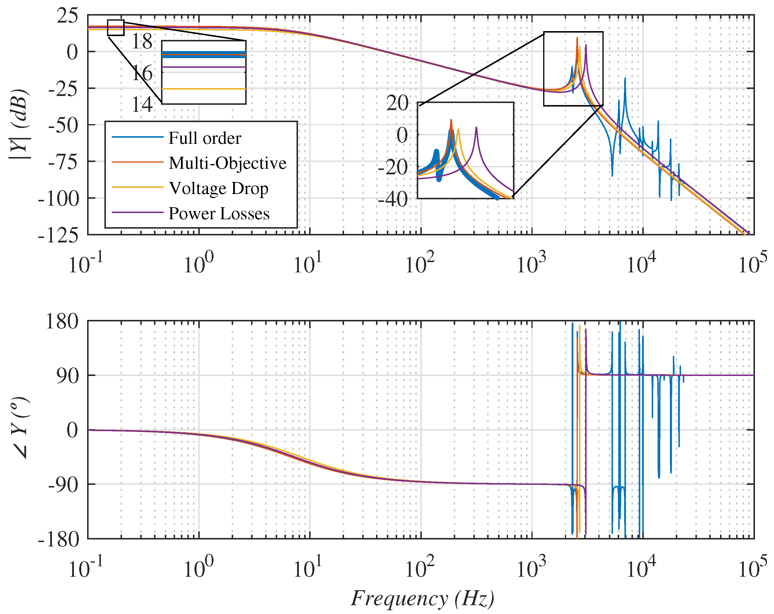
Figure 6 shows the WPP grid admittance as a function of the frequency of the complete 150-state SISO model, as well as that of each one of the aggregated models (multi-objective optimization, voltage drop, and power losses’ aggregation). All aggregation techniques showed a relative good agreement with the detailed model admittance for a wide range of frequencies.

However, the proposed technique showed a much closer match of low frequency admittance values and, more importantly, an excellent match of both main resonant peak frequency and amplitude. It is worth noting that both voltage drop- and power loss-based aggregation showed main resonant peak frequencies that were far off from the actual resonant peak. The largest error was obtained from the power loss error, which led to a resonant peak frequency of more than 500 Hz higher than its actual value.

Additionally, different WPP topologies have been studied, in order to verify that the proposed aggregation technique is valid for different WPP configurations. The studies covered different numbers of connected strings and also different numbers of connected WTGs per string. In all cases, the multi-objective aggregation technique always showed a better admittance frequency response match than the other two considered aggregation techniques.

Clearly, the results in Figure 6 represent small signal operation; however, the proposed aggregation technique had a very good agreement with the actual grid admittance for a very wide range of frequencies, including the main resonant peak. Therefore, the proposed aggregation technique is expected to show dynamic characteristics very close to the detailed 150-state system. The dynamic response of the proposed and state-of-the-art techniques is covered in Section 6.

6. Results

The frequency results in Figure 6 suggest that the proposed aggregation method should be able to represent the full system dynamics with less error than the other two considered aggregation techniques. Therefore, the EMTsimulation of the considered test cases was carried out in order to verify the dynamic behavior of each aggregation method.

Four scenarios have been considered, one with full detail models of each cluster (considering the full 150 WTGs of 8 MW each), and considering an aggregated equivalent for each one of the three 400-MW clusters (with multi-objective optimization, voltage drop, and power losses’ aggregation methods).

The PSCAD-EMT simulations for the system shown in Figure 3 have been carried out in all four scenarios considered. However, for the sake of clarity, only the full simulation results corresponding to the detailed and multi-objective aggregated model are shown in the simulation section. The results corresponding to the other two aggregation methods are shown as errors with respect to the detailed model simulations.

The validation of the aggregated models has been carried out by comparing the active and reactive power and voltage and current ($P_{Fk}$, $Q_{Fk}$, $V_{Fk}$, $I_{Fk}$) responses at the points of common coupling of each one of the wind power plants (buses PCC${}_{1,2,3}$ in Figure 3).

Three test cases have been considered:

• Fast changes in active power reference.
• Disconnection of one of the three wind power plants.
• Disconnection and re-connection of diode rectifier station AC filters.

Finally, a study of the computational load of each alternative has been carried out.

6.1. Simulation Results

6.1.1. Case 1: Fast Changes in Active Power Reference

The three wind power plants were initially operated in islanding mode (DR not conducting) with a voltage reference of $0.87$ pu. From this state, the active power reference was ramped up from 0–1 pu in 150 ms for all three WPPs at the same time. Once all the WPPs reached their steady state operation, several step transients on active power reference were applied from 1 down to $0.5$ pu, by sequentially reducing the active power reference $P_{Fk}^{*}$ of each individual wind power plant.

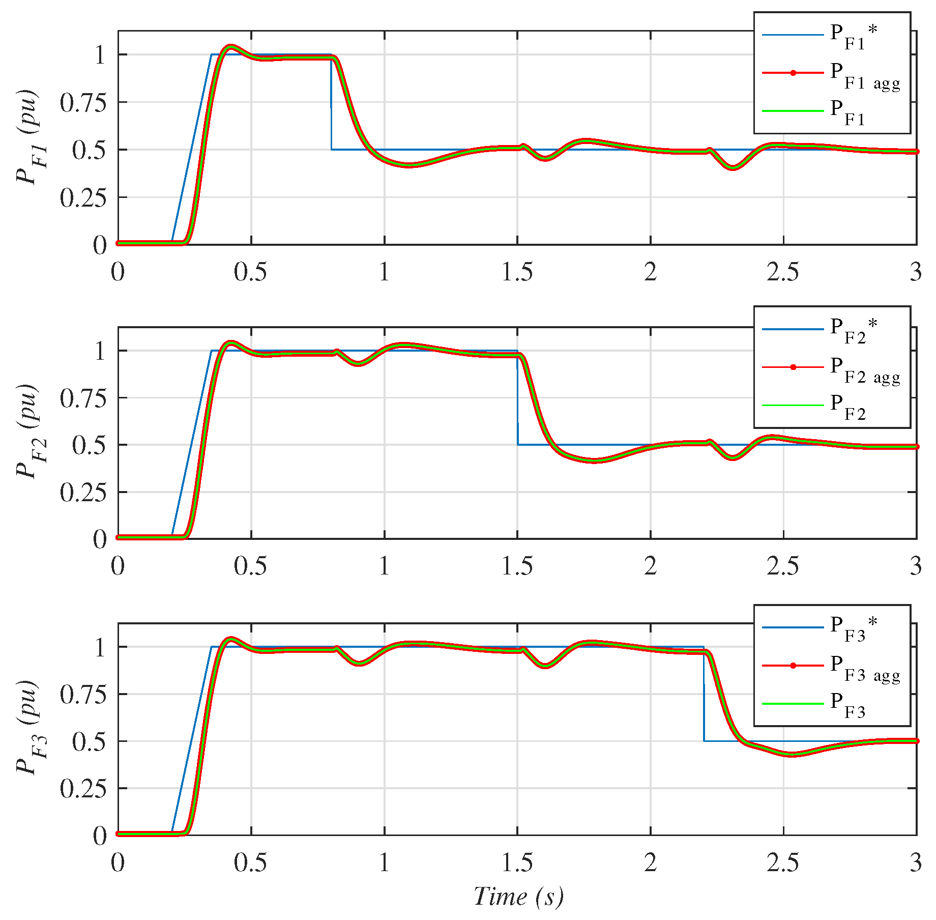
Figure 7 shows the behavior of the active power $P_{Fk}$. Initially, the active power reference $P_{Fk}^{*}$ rose to 1 pu at $t=0.2$ s, but power production did not increase until currents began to flow through the DR at $t=0.25$ s. The reason for this is that the AC-side DR voltage had to be higher than $0.9$ pu for the DR station to start conducting. Then, at $t=0.8$ s, the active power reference $P_{Fk}^{*}$ was decreased to $0.5$ pu in each cluster every $0.7$ s. Such rapid active power transients might not be realistic, but have been chosen as an extreme case for validation purposes. Figure 7 clearly shows that both aggregated and detailed models led to very similar active power dynamic results.

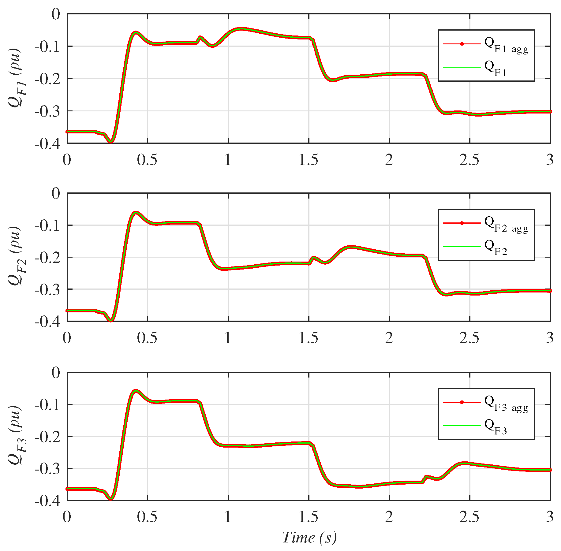
Figure 8 shows the reactive power responses for each WPP $Q_{Fk}$. The reactive power produced by the AC filters was compensated by the WTGs while DRs were not delivering power. Conversely, when the DRs started conducting, the capacitor and AC filter banks’ reactive power compensated that absorbed by the DRs, and hence, the reactive power $Q_{Fk}$ delivered by the wind farms was reduced to a value very close to zero. Reactive power ($Q_{Fk}$) responses were also very similar for both aggregated and detailed models.

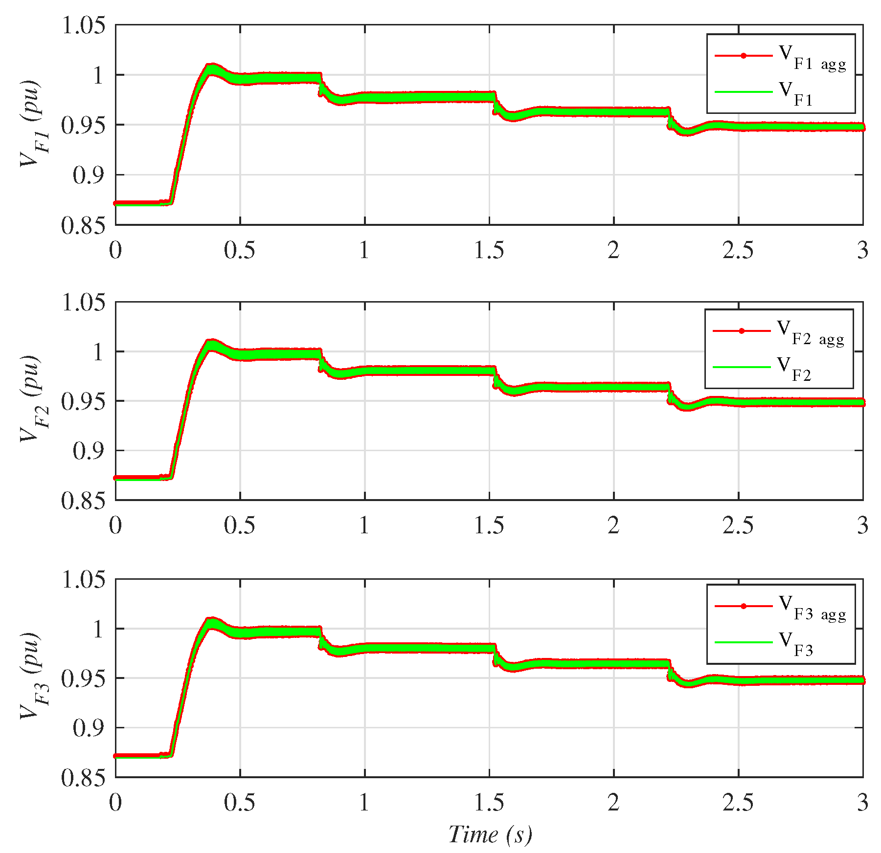
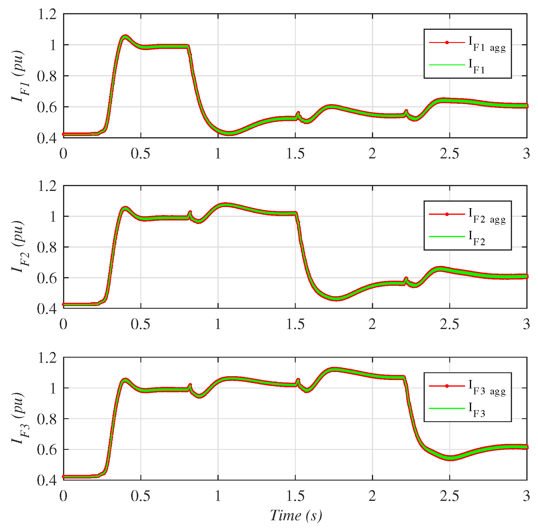
Figure 9 shows the behavior of the voltage $V_{Fk}$ at the PCC of each WPP. It shows clearly how active power flow by DRs depends of the voltage $V_{Fk}$. Figure 10 shows the magnitudes of current $I_{Fk}$ at the PCC of each WPP. The current behavior was similar to that of the active power $P_{Fk}$. Figure 9 and Figure 10 clearly show that the voltage and current dynamics from the aggregated and detailed models agree to a great extent.

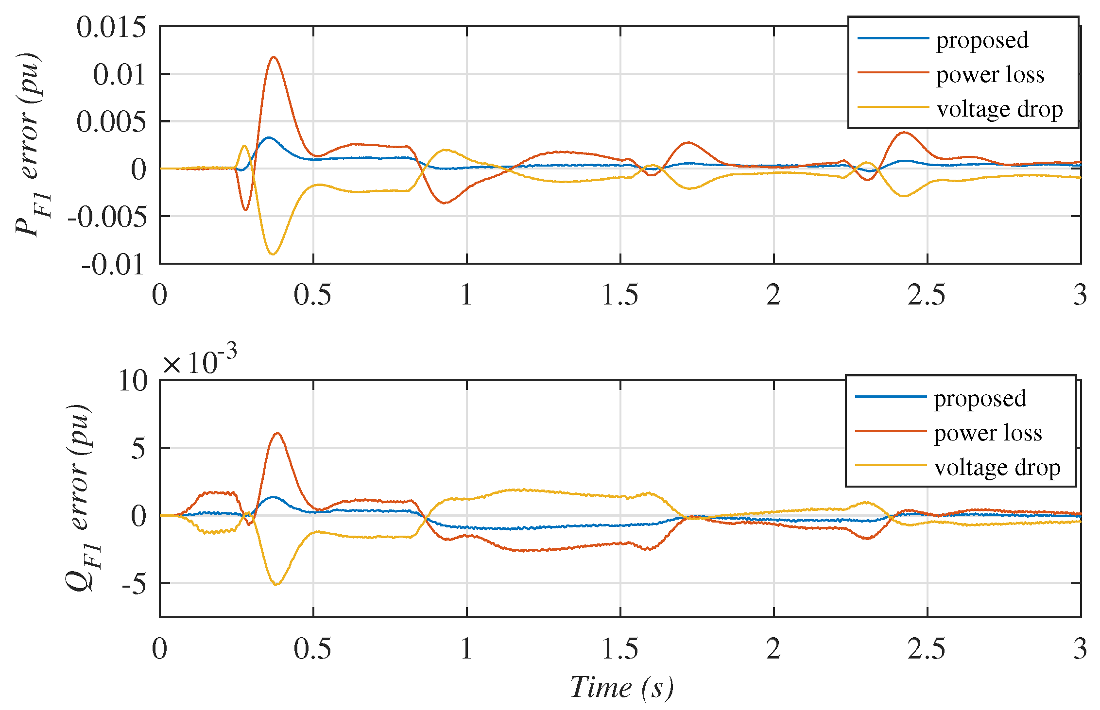
Three aggregation methods have been used to simulate the fast active power transients considered in Case 1. The results are shown in Figure 11, which shows the active and reactive power simulation errors between aggregated and detailed models at PCC-1, i.e., ($P_{F1Detailed}-P_{F1Agg}$) and ($Q_{F1Detailed}-Q_{F1Agg}$). Only the traces corresponding to PCC-1 are shown, as the other PCCs showed a very similar behavior.

The simulation error obtained using the proposed multi-objective optimization aggregation technique (in blue in Figure 11) was clearly lower than those with the alternative aggregation techniques.

The maximum active power simulation error with the proposed technique was about $0.3\%$, whereas the maximum simulation error for the reactive power simulation was approximately $0.2\%$. For the power loss technique, the active and reactive power maximum simulation errors were $0.9\%$ and $0.5\%$, respectively, whereas for the voltage drop technique for the maximum simulation, the corresponding errors were $1.2\%$ and $0.7\%$. Therefore, the proposed technique clearly showed a more accurate simulation during transients.

Moreover, for the complete case, the error variance using the multi-objective optimization aggregation technique was $0.0423$, whereas the error variance with the voltage droop and power losses techniques was $0.4094$ and $0.3120$, respectively. Therefore, the error variance for the proposed technique was up to $9.5$-times better than the other aggregation techniques.

6.1.2. Case 2: Wind Power Plant Disconnection

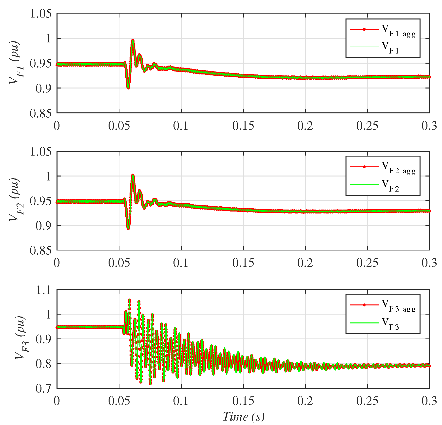
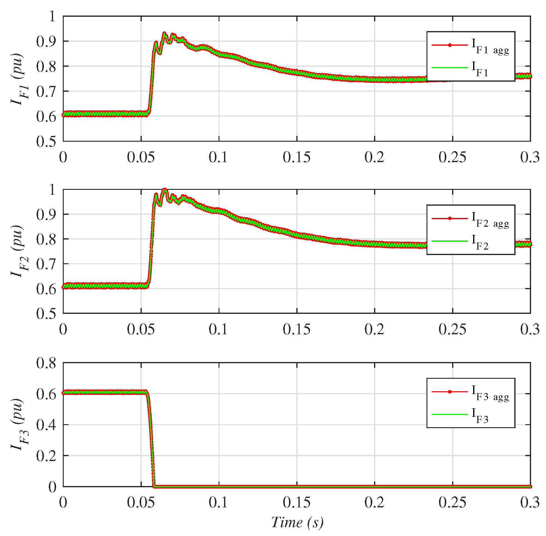
The second test case consisted of the disconnection of WPP3, by opening the breaker at $V_{F3}$ in Figure 3 at t = 0.05 s. Initially, all WPPs were generating 0.5 pu rated power. Figure 12 and Figure 13 show the behavior of the WPP voltage and current magnitude at the PCC of each wind power plant.

After disconnection, WPP3’s voltage remained at its 0.8 pu reference value, as all considered WTGs were grid-forming (Figure 12). After the transient, the voltage of the WPPs that remained connected settled to a slightly smaller voltage, as the power transmitted through the diode rectifiers was now reduced by one third [5].

From Figure 12 and Figure 13, it is clear that voltage and currents obtained from the detailed and from the proposed aggregated models showed an excellent agreement during the transient.

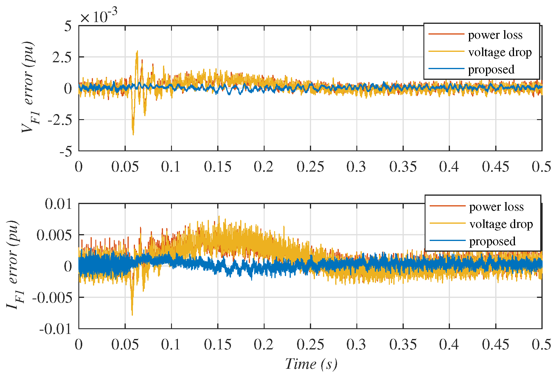
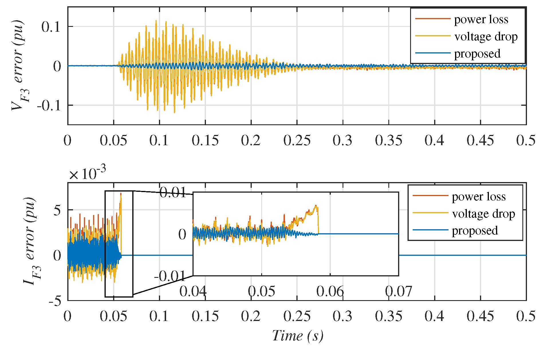
The same WPP3 disconnection case shown in Figure 12 and Figure 13 has been repeated considering two alternative aggregation techniques (power loss and voltage drop). The results are shown in Figure 14 and Figure 15, which show the difference between the detailed simulation and each one of the three considered aggregation techniques. Simulation errors are expressed as per unit with respect to rated values.

Figure 14 shows the errors on the simulated voltages and currents for the detailed and aggregated models, $(V_{F1Detailed}-V_{F1Agg})$ and $(I_{F1Detailed}-I_{F1Agg})$ respectively. These voltages and currents correspond to one of the two WPP that was not disconnected (WPP1). The proposed aggregation technique (in blue) clearly showed a better performance than existing aggregation techniques, although all aggregation techniques showed relatively small $V_{F1}$ and $I_{F1}$ simulation errors.

However, the voltage and current transients were much larger in the disconnected WPP3, as previously shown in Figure 12 and Figure 13. The top graph of Figure 15 shows that the $V_{F3}$ simulation error for the proposed aggregation method was much smaller than that of the existing aggregation methods (which even reached simulation errors larger than 10%).

On the other hand, the $I_{F3}$ simulation errors were very small for all aggregation techniques, with only a small deviation just at the instant of WPP3 disconnection (Figure 15 bottom graph).

6.1.3. Case 3: Disconnection and Re-Connection of Diode Rectifier AC Filters

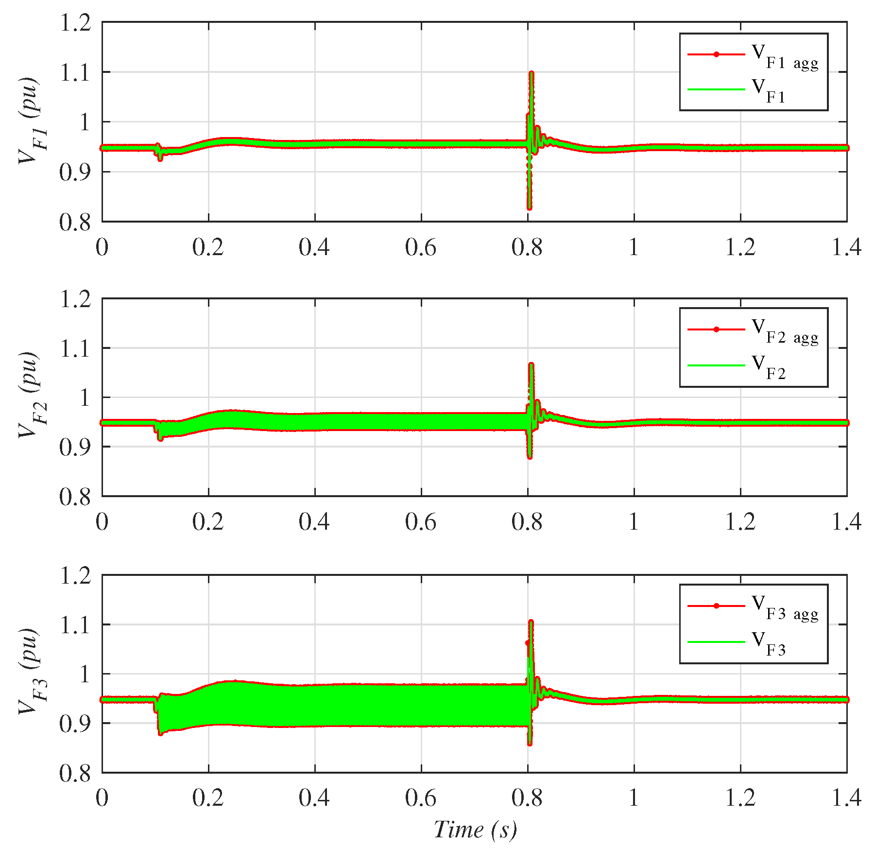
The third case consisted of the disconnection and re-connection of the AC capacitor and filter banks of DRU${}_3$(Figure 3). The capacitor and filter banks of each DRU were rated at 0.4 pu (160 MVAr) and were connected in several steps. However, this transient considered the connection and disconnection of the full AC filter banks, in order to validate the dynamic performance of the aggregated models.

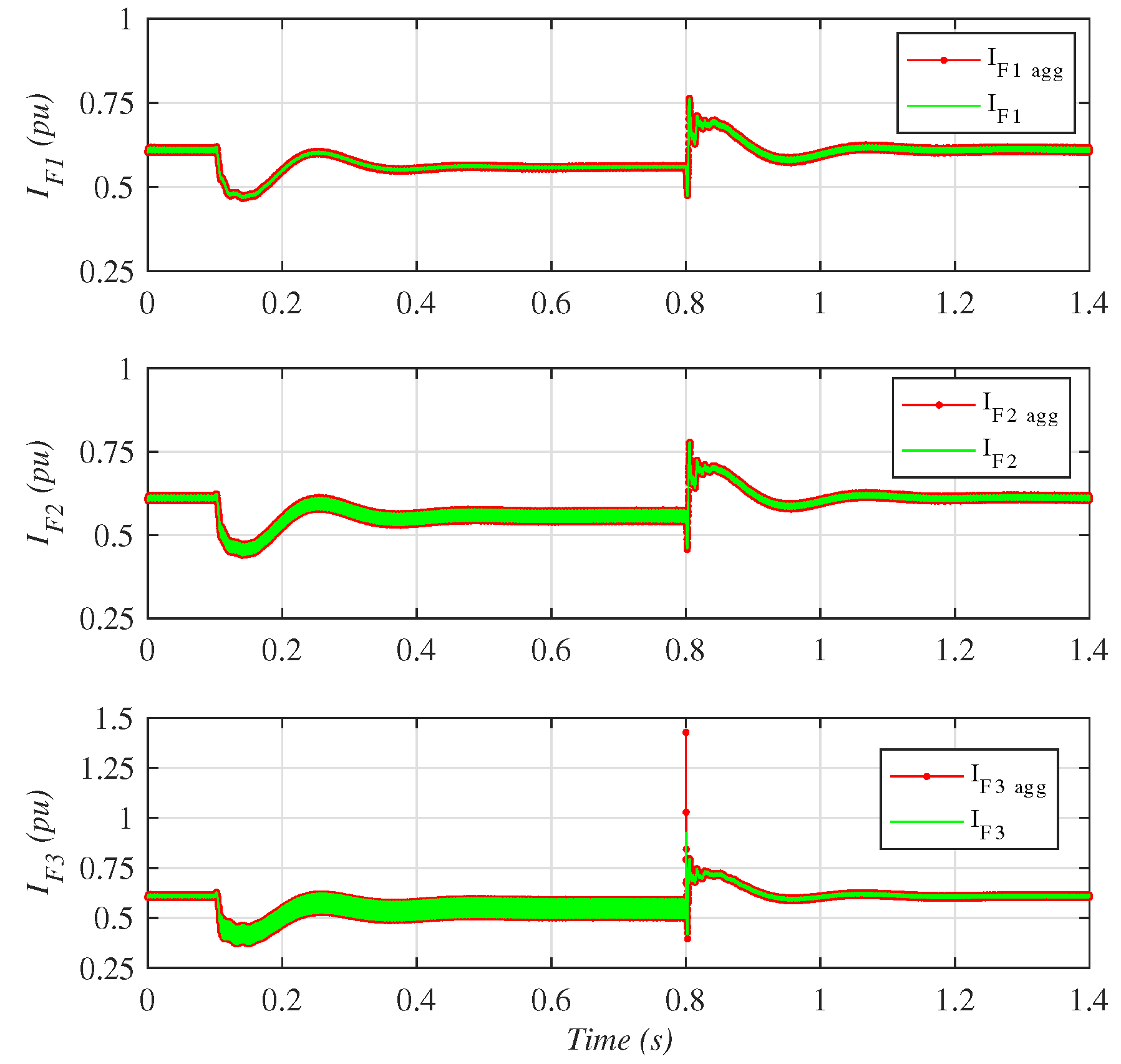
The voltages and current output of each WPP during this test case are shown in Figure 16 and Figure 17. The DRU${}_3$ AC filter banks were disconnected at t = 0.1 s and re-connected at t = 0.8 s. Clearly, the harmonic contents of both voltage and current increased when the filter banks were disconnected. Moreover, voltage and current distortion was larger for WPP3, as it was electrically closer to the DRU station with no AC filters connected. WPP1 showed a relatively small voltage and current ripple when the filters were disconnected, whereas WPP2 showed intermediate harmonic contents.

In any case, there was a very large agreement between detailed and aggregated simulations during the complete transient, except for the large current peak during AC filter bank reconnection in $I_{F3}$ at t = 0.8 s (Figure 17), where the aggregated model overestimated the $I_{F3}$ current peak.

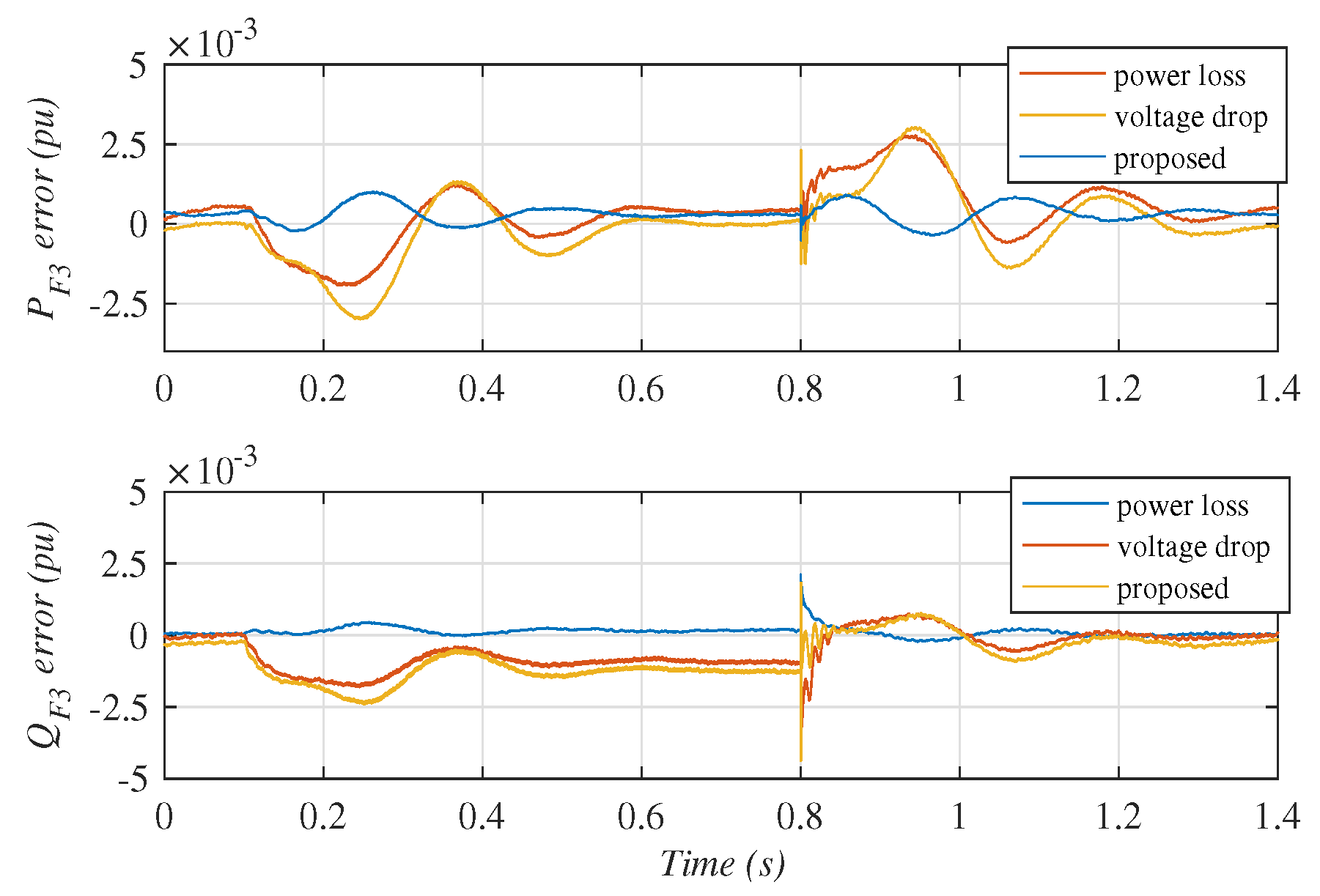
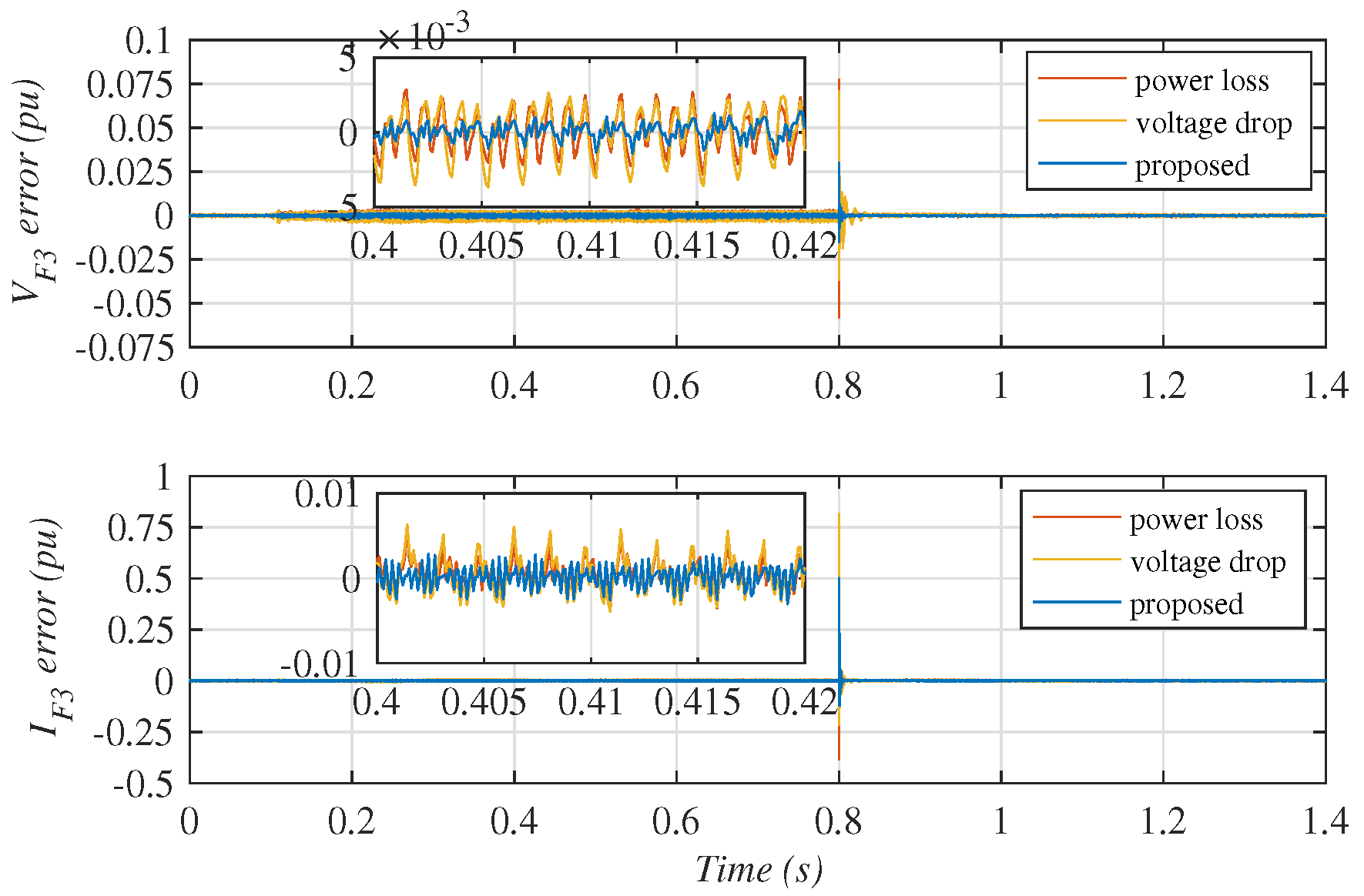
The comparison of the proposed aggregation technique with existing techniques is shown in Figure 18 and Figure 19. These figures show the simulation errors for the three aggregation techniques, during the DRU${}_3$ AC filter disconnection and re-connection transient considered in this section.

Figure 18 shows the error on WPP3 active and reactive powers ($P_{F3}$ and $Q_{F3}$) when simulated with each one of the considered aggregation techniques. All aggregation models adequately simulated the steady state active and reactive power delivered by WPP3. However, it was clear that, during the transients, the proposed aggregation technique (shown in blue) showed a smaller simulation error than existing techniques.

Figure 19 (top graph) shows that the proposed aggregation technique also showed a smaller $V_{F3}$ error than other techniques when the filters were disconnected (i.e., between t = 0.1 and t = 0.8 s). Clearly, the proposed technique was relatively better at simulating $V_{F3}$ voltage harmonics.

On the other hand, Figure 19 (bottom graph) shows that current $I_{F3}$ simulation errors between t = 0.1 and t = 0.8 s were very similar for the three considered techniques, around 0.5% (albeit that the proposed technique error was slightly better).

It is worth noting that all aggregation techniques showed relatively large simulation errors for $V_{F3}$ and $I_{F3}$ when the AC filter banks were re-connected at t = 0.8 s (Figure 19). However, the proposed technique performed clearly better than voltage drop and power loss aggregation techniques.

6.2. Simulation Performance

The simulations of all considered cases have been carried out with a 3.3-GHz Intel Core i7 PC with 16 GB DDR3 memory, SSD hard drive, and MS-Windows 7.

Considering a simulation run time of 3 s,

Table 2. Simulation times.

	WTGs	Nodes	Simulation Time
Detailed	150	2450	117 min
Aggregated	3	174	20 s

shows the complexity and simulation times of both detailed and aggregated models. The detailed simulation took 2 h, whereas the aggregated simulation was more than 350-times faster.

Therefore, the use of the proposed aggregated models for large Type-4 wind power plants was validated considering the similarity of the obtained results and the improvement on simulation times.

7. Discussion and Conclusions

This paper has presented an aggregation approach based on model order reduction using a multi-objective optimization technique. The proposed method consisted of first obtaining full admittance model of the WPP (in our case using state space techniques), then the inputs to the system were reduced to a single input applying the superposition principle, and finally, multi-objective optimization has been used to reduce the order of the system. The proposed aggregation technique considered voltage source WTGs’ line side converters; therefore, it is also applicable to current-controlled voltage source converters.

Using the multi-objective optimization aggregation technique, the achieved aggregated admittance model had the same DC gain, main resonant frequency, and the same gain at the operating frequency as the detailed admittance model.

The proposed aggregation technique was validated considering the PSCAD/EMTDC simulation of a 1.2-GW HVDC DR-connected system, consisting of three 400-MW WPP of 50 Type-4 grid-forming WTGs each. Hence, the detailed system consisted of 150 individual wind turbines and 2450 nodes.

The proposed aggregation technique and two commonly-used aggregation strategies have been used to reduce the WPPs to only three aggregated WPPs (each one equivalent to 400 MW).

The comparison has been carried out considering three different test cases, namely fast active power reference changes, disconnection of a wind power plant, and disconnection and re-connection of DRU AC filter banks. These cases cover a wide range of dynamic and transient conditions.

The response against active power changes achieved by using the proposed aggregation method showed a worst case error three-times and an error variance $9.5$-times better than aggregation techniques based on voltage drop or on power losses.

During WPP disconnection, all aggregation techniques showed relatively good PCC voltage and current simulation accuracy for the two wind power plants that remained connected. However, for the disconnected WPP, the proposed method showed voltage simulation accuracy 10-times better than standard methods, during the disconnection transient.

During disconnection and re-connection of one of the DRU AC filter banks, the proposed technique also showed better simulation accuracy regarding PCC voltage, active, and reactive power.

Finally, it has been shown that the aggregated simulations were 350-times faster than their detailed counterpart.

Therefore, when only the behavior at the points of common coupling is of interest, the proposed aggregated model provides important simulation time savings while delivering accurate results and preserving the main resonant characteristics of the full array system.

References

- Menke, P. New Grid Access Solutions for Offshore Wind Farms; EWEA Off-Shore: Copenhagen, Denmark, 2015. [Google Scholar]
- Blasco-Gimenez, R.; Añó-Villalba, S.; Rodríguez, J.; Morant, F.; Bernal, S. Uncontrolled rectifiers for HVDC connection of large off-shore wind farms. In Proceedings of the 13th European Conference on. Power Electronics and Applications, Barcelona, Spain, 8–10 September 2009; pp. 1–8. [Google Scholar]
- Blasco-Gimenez, R.; Añó-Villalba, S.; Rodríguez-D’Derlée, J.; Morant, F.; Bernal-Perez, S. Distributed Voltage and Frequency Control of Offshore Wind Farms Connected With a Diode-Based HVDC Link. IEEE Trans. Power Electron. 2010, 25, 3095–3105. [Google Scholar] [CrossRef]
- Blasco-Gimenez, R.; Añó-Villalba, S.; Rodriguez-D’Derlée, J.; Bernal-Perez, S.; Morant, F. Diode-Based HVDC Link for the Connection of Large Offshore Wind Farms. IEEE Trans. Energy Convers. 2011, 26, 615–626. [Google Scholar] [CrossRef]
- Bernal-Perez, S.; Añó-Villalba, S.; Blasco-Gimenez, R.; Rodriguez-D’Derlee, J. Efficiency and Fault Ride-Through Performance of a Diode-Rectifier- and VSC-Inverter-Based HVDC Link for Offshore Wind Farms. IEEE Trans. Ind. Electron. 2013, 60, 2401–2409. [Google Scholar] [CrossRef]
- Blasco-Gimenez, R.; Aparicio, N.; Añó-Villalba, S.; Bernal-Perez, S. LCC-HVDC Connection of Offshore Wind Farms With Reduced Filter Banks. IEEE Trans. Ind. Electron. 2013, 60, 2372–2380. [Google Scholar] [CrossRef]
- Kocewiak, L.H. Harmonics in Large Offshore Wind Farms. Ph.D. Thesis, Department of Energy Technology, Aalborg University, Aalborg, Denmark, 2012. [Google Scholar]
- Kocewiak, L.H.; Hjerrild, J.; Bak, C.L. Wind turbine converter control interaction with complex wind farm systems. IET Renew. Power Gener. 2013, 7, 380–389. [Google Scholar] [CrossRef]
- Muljadi, E.; Butterfield, C.P.; Ellis, A.; Mechenbier, J.; Hochheimer, J.; Young, R.; Miller, N.; Delmerico, R.; Zavadil, R.; Smith, J.C. Equivalencing the collector system of a large wind power plant. In Proceedings of the 2006 IEEE Power Engineering Society General Meeting, Montreal, QC, Canada, 18–22 June 2006. [Google Scholar]
- Garcia-Gracia, M.; Comech, M.P.; Sallan, J.; Llombart, A. Modeling wind farms for grid disturbance studies. Renew. Energy 2008, 33, 2109–2121. [Google Scholar] [CrossRef]
- Fernandez, L.M.; Garcia, C.A.; Saenz, J.R.; Jurado, F. Equivalent models of wind farms by using aggregated wind turbines and equivalent winds. Energy Convers. Manag. 2009, 50, 691–704. [Google Scholar] [CrossRef]
- Brogan, P. The stability of multiple, high power, active front end voltage sourced converters when connected to wind farm collector systems. In Proceedings of the EPE Wind Energy Chapter Seminar, Brno, Czech Republic, 4–6 May 2010; pp. 1–6. [Google Scholar]
- Kocewiak, L.H.; Hjerrild, J.; Bak, C.L. Wind farm structures’ impact on harmonic emission and grid interaction. In Proceedings of the European Wind Energy Conference & Exhibition, Warsaw, Poland, 20–23 April 2010. [Google Scholar]
- Martínez-Turégano, J.; Añó-Villalba, S.; Chaques-Herraiz, G.; Bernal-Perez, S.; Blasco-Gimenez, R. Model aggregation of large wind farms for dynamic studies. In Proceedings of the IECON 2017—43rd Annual Conference of the IEEE Industrial Electronics Society, Beijing, China, 29 October–1 November 2017; pp. 316–321. [Google Scholar]
- Semlyen, A.; Deri, A. Time Domain Modeling of Frequency Dependent Three-Phase Transmission Line Impedance. IEEE Trans. Power Appar. Syst. 1985, PAS-104, 1549–1555. [Google Scholar] [CrossRef]
- Garcia, N.; Acha, E. Transmission line model with frequency dependency and propagation effects: A model order reduction and state-space approach. In Proceedings of the 2008 IEEE Power and Energy Society General Meeting—Conversion and Delivery of Electrical Energy in the 21st Century, Pittsburgh, PA, USA, 20–24 July 2008; pp. 1–7. [Google Scholar]
- Beerten, J.; D’Arco, S.; Suul, J.A. Frequency-dependent cable modelling for small-signal stability analysis of VSC-HVDC systems. IET Gener. Transm. Distrib. 2016, 10, 1370–1381. [Google Scholar] [CrossRef]
- Ruiz, C.; Abad, G.; Zubiaga, M.; Madariaga, D.; Arza, J. Frequency-Dependent Pi Model of a Three-Core Submarine Cable for Time and Frequency Domain Analysis. Energies 2018, 11, 2778. [Google Scholar] [CrossRef]
- Brayton, R.; Director, S.; Hachtel, G.; Vidigal, L. A new algorithm for statistical circuit design based on quasi-Newton methods and function splitting. IEEE Trans. Circuits Syst. 1979, 26, 784–794. [Google Scholar] [CrossRef]
- Gembicki, F.W. Vector Optimization for Control with Performance and Parameter Sensitivity Indices. Ph.D. Thesis, Case Western Reserve University, Cleveland, OH, USA, 1974. [Google Scholar]
- Fleming, P.J. Computer aided control system design using a multi-objective optimization approach. In Proceedings of the Control 1985 Conference, Cambridge, UK, 22 January 1985; pp. 174–179. [Google Scholar]
- Han, S.P. A globally convergent method for nonlinear programming. J. Optim. Theory Appl. 1977, 22, 297–309. [Google Scholar] [CrossRef]
- Guerrero, J.M.; Vasquez, J.C.; Matas, J.; de Vicuna, L.G.; Castilla, M. Hierarchical Control of Droop-Controlled AC and DC Microgrids—A General Approach Toward Standardization. IEEE Trans. Ind. Electron. 2011, 58, 158–172. [Google Scholar] [CrossRef]
- Szechtman, M.; Wess, T.; Thio, C.V. First benchmark model for HVDC control studies. Electra 1991, 135, 54–73. [Google Scholar]
Figure 1.
WTG-j () in the string-i () of the wind power plant (WPP).
Figure 2.
Model of an aggregated WPP.
Figure 3.
Off-shore WPP with three WPPs of 400 MW each connected to the on-shore grid through a diode-based HVDC link.
Figure 4.
Left: centralized power control; right: distributed droop controls.
Figure 5.
Hankel singular values (state contributions; the first 20 states are shown).
Figure 6.
WPP grid admittance as a function of frequency: blue: 150 order system; red: multi-objective optimization; yellow: voltage drop; purple: power loses.
Figure 7.
Case 1—Active power at PCC-k of each diode rectifier platform for detailed and aggregated models.
Figure 8.
Case 1—Reactive power at PCC-k of each diode rectifier platform for the detailed and aggregated models.
Figure 9.
Case 1—Voltage amplitude at the PCC of each WPP () for detailed and aggregated models.
Figure 10.
Case 1—Current amplitude at the PCC of each WPP () for detailed and aggregated models.
Figure 11.
Case 1—Simulation errors for different aggregation techniques: top: ; bottom: .
Figure 12.
Case 2—Comparison of detailed and proposed aggregated simulations. WPP voltage .
Figure 13.
Case 2—Comparison of detailed and proposed aggregated simulations. WPP current .
Figure 14.
Case 2—Simulation errors for different aggregation techniques: top: ; bottom: .
Figure 15.
Figure 16.
Case 3—Comparison of detailed and proposed aggregated simulations. WPP voltage .
Figure 17.
Figure 18.
Case 3—Simulation errors for different aggregation techniques: top: ; bottom: .
Figure 19.