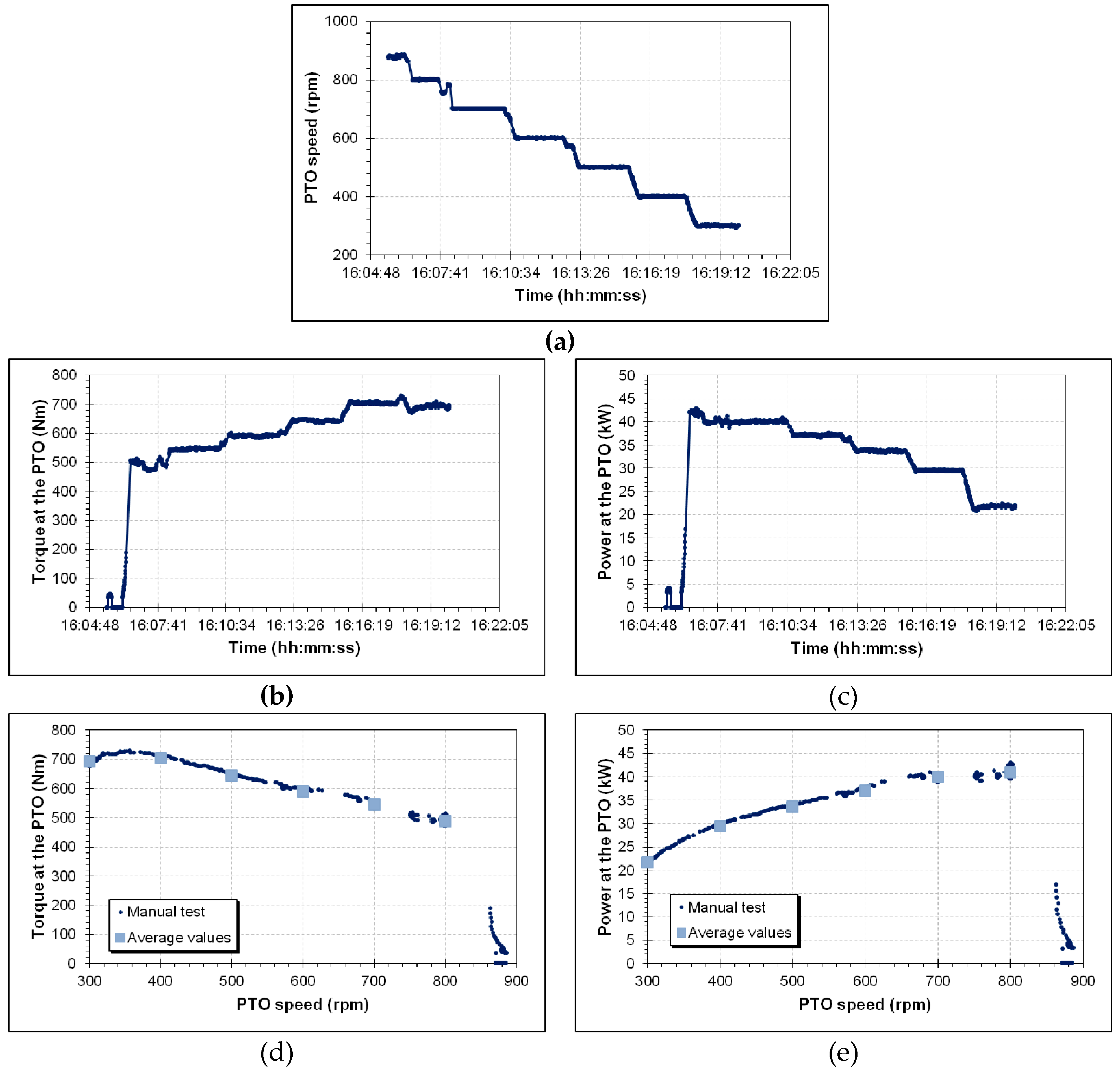
Figure 1.
Examples of outputs from the PTO-dyno during a (speed-controlled) manual test on the New Holland T4020V farm tractor fuelled with pure pump diesel oil (D100); (top) temporal trends of PTO speed (a), torque (b) and power (c); (bottom) positioning of the experimental points in a “torque vs. speed” (d) and “power vs. speed” space (e).
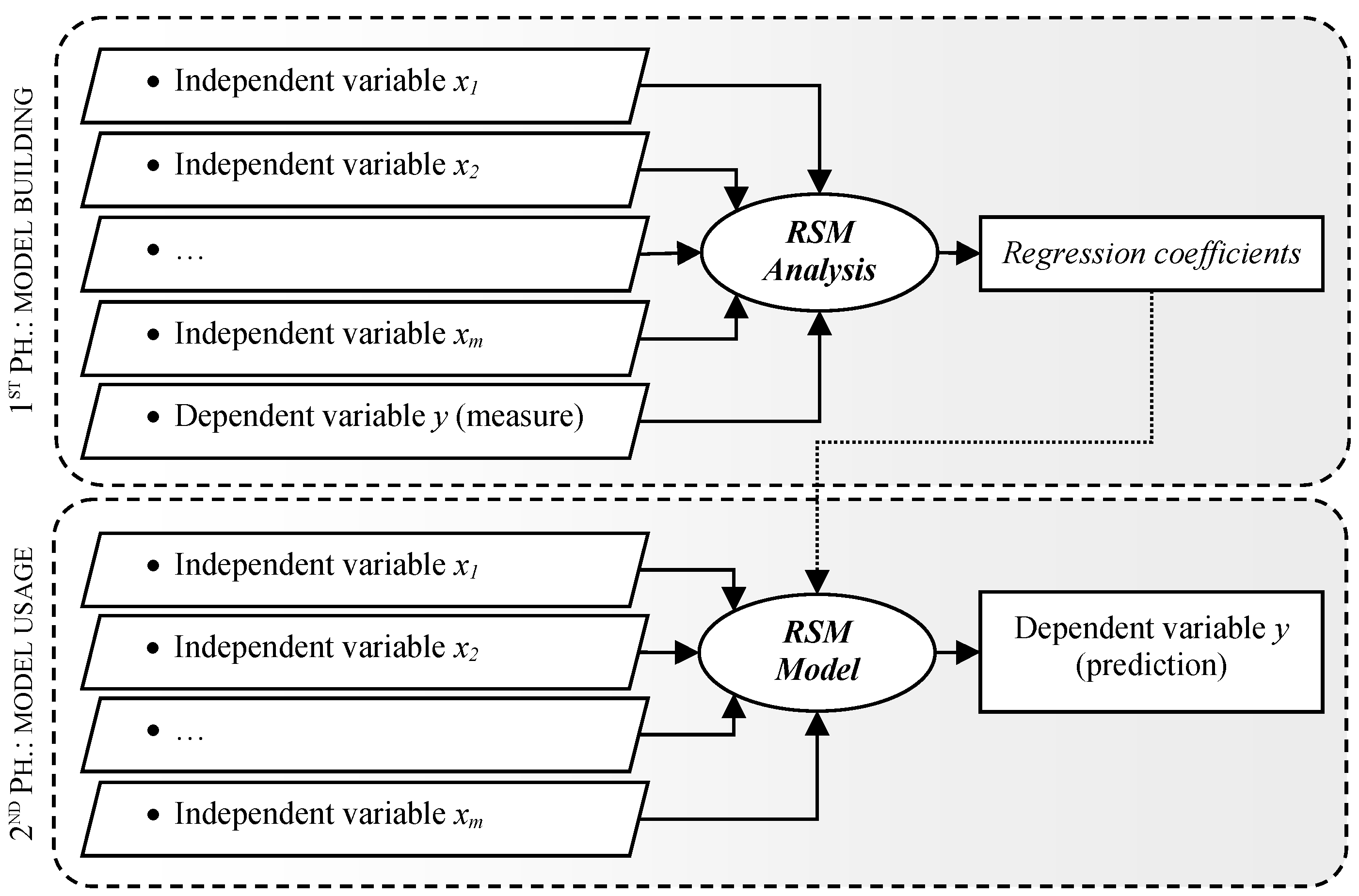
Figure 2.
General procedure of use of experimental data to build a model later useful to indirectly forecast the values of an independent variable y, given the values of m dependent variables xi. (parallelograms/rectangles: input/output quantities; ellipses: tools involved in the computations).
Figure 2.
General procedure of use of experimental data to build a model later useful to indirectly forecast the values of an independent variable y, given the values of m dependent variables xi. (parallelograms/rectangles: input/output quantities; ellipses: tools involved in the computations).
Figure 3.
Detailed list of all technical characteristics, machine settings and other quantities (independent variables; on the left) fixing the operative point of a tractor involved in performing a task, defined by the engine speed and a certain level of power delivered by the engine, of consumptions, of CO, NOx and particulate matter in its exhaust gases (dependent variables; on the right).
Figure 4.
Variables considered in the assessment of the performances of the tested tractor (model including the composition of the fuel blends).
Figure 4.
Variables considered in the assessment of the performances of the tested tractor (model including the composition of the fuel blends).
Figure 5.
Variables considered in the assessment of the performances of the tested tractor (models including the kinematic viscosity of the fuel blends).
Figure 5.
Variables considered in the assessment of the performances of the tested tractor (models including the kinematic viscosity of the fuel blends).
Figure 6.
Procedure followed in the application of the Response Surface Methodology (RSM) approach to the experimental data.
Figure 6.
Procedure followed in the application of the Response Surface Methodology (RSM) approach to the experimental data.
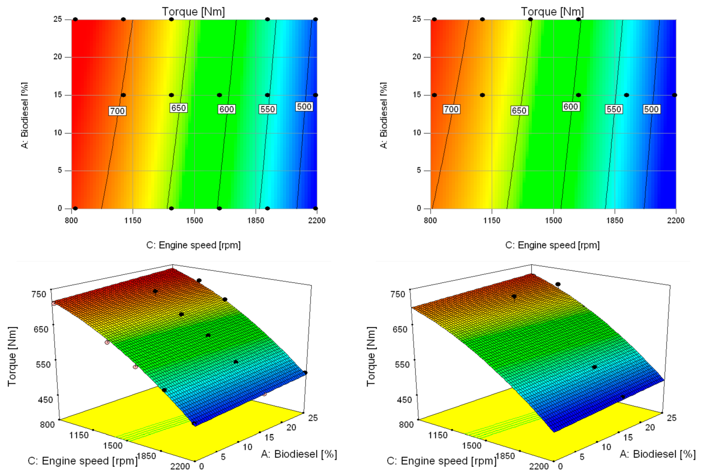
Figure 7.
Contour plots (top) and 3D-graphs (bottom) of the engine torque as a function of the biodiesel percentage and of the engine speed referred to the 1st model (24 cases), with the 0% (left) and the 3% (right) of bioethanol in the blend (NB: the values of torque are reported as labels directly on the contours). The same pictures show also the positions of the experimental measurements (black dots positioned within the investigated hyperspace; notice that many points are positioned under the represented surface and hence are not visible).
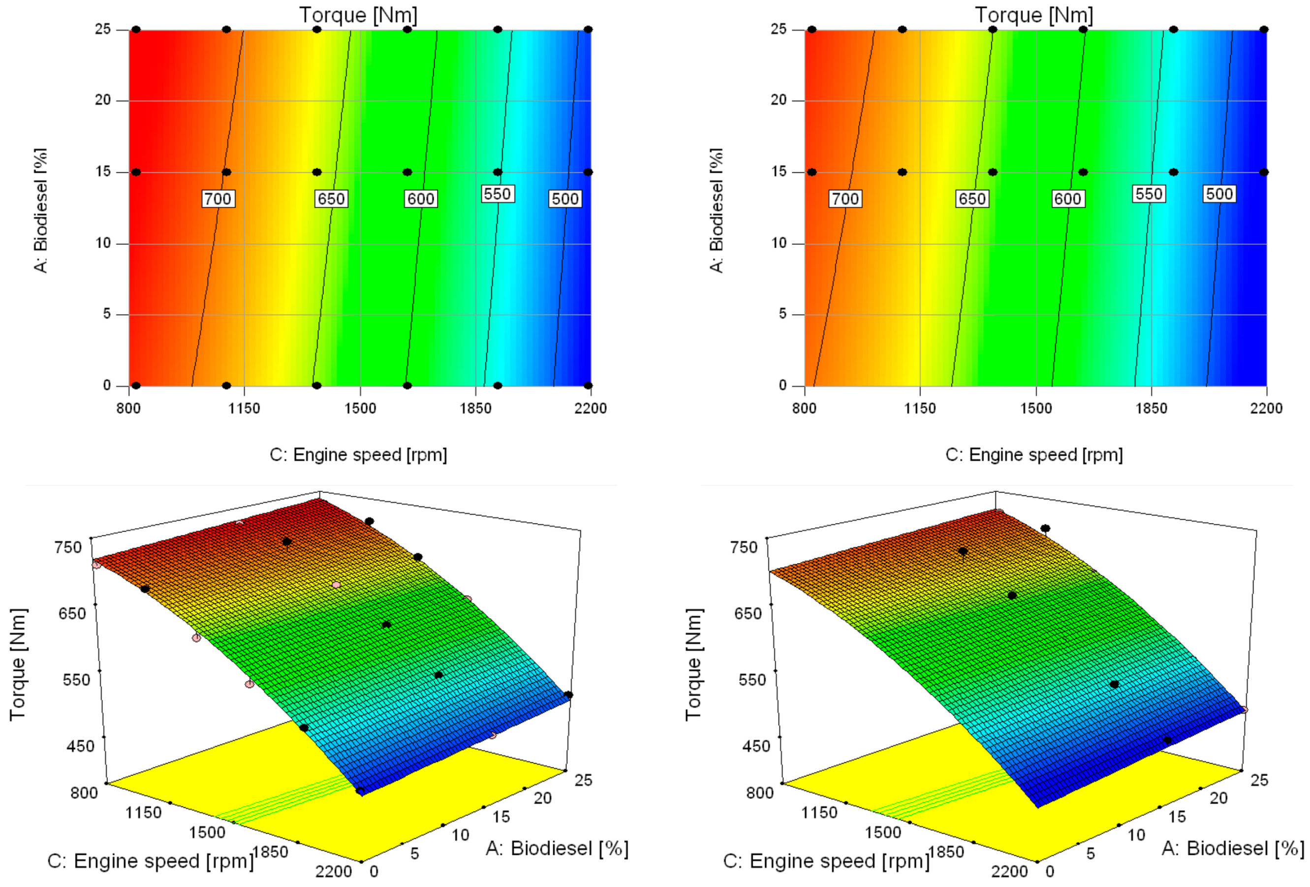
Figure 8.
Contour plots (top) and 3D-graphs (bottom) of the engine torque as a function of the biodiesel percentage and of the engine speed referred to the 2nd model (30 cases), with the 0% (left) and the 3% (right) of bioethanol in the blend (NB: the values of torque are reported as labels directly on the contours). The same pictures show also the positions of the experimental measurements (black dots positioned within the investigated hyperspace; notice that many points are positioned under the represented surface and hence are not visible).
Figure 9.
Contour plots (top) and 3D-graphs (bottom) of the hourly fuel consumption at full load as a function of the biodiesel percentage and of the engine speed referred to the 1st model (24 cases), with the 0% (left) and the 3% (right) of bioethanol in the blend (NB: the values of hourly consumption are reported as labels directly on the contours). The same pictures show also the positions of the experimental measurements (black dots positioned within the investigated hyperspace; notice that many points are positioned under the represented surface and hence are not visible).
Figure 10.
Contour plots (top) and 3D-graphs (bottom) of the hourly fuel consumption at full load as a function of the biodiesel percentage and of the engine speed referred to the 2nd model (30 cases), with the 0% (left) and the 3% (right) of bioethanol in the blend (NB: the values of hourly consumption are reported as labels directly on the contours). The same pictures show also the positions of the experimental measurements (black dots positioned within the investigated hyperspace; notice that many points are positioned under the represented surface and hence are not visible).
Figure 11.
Contour plots (top) and 3D-graphs (bottom) of the NOx concentration as a function of the biodiesel percentage and of the engine speed referred to the 1st model (24 cases), with the 0% (left) and the 3% (right) of bioethanol in the blend (NB: the values of NOx are reported as labels directly on the contours). The same pictures show also the positions of the experimental measurements (black dots positioned within the investigated hyperspace; notice that many points are positioned under the represented surface and hence are not visible).
Figure 12.
Contour plots (top) and 3D-graphs (bottom) of the NOx concentration as a function of the biodiesel percentage and of the engine speed referred to the 2nd model (30 cases), with the 0% (left) and the 3% (right) of bioethanol in the blend (NB: the values of NOx are reported as labels directly on the contours). The same pictures show also the positions of the experimental measurements (black dots positioned within the investigated hyperspace; notice that many points are positioned under the represented surface and hence are not visible).
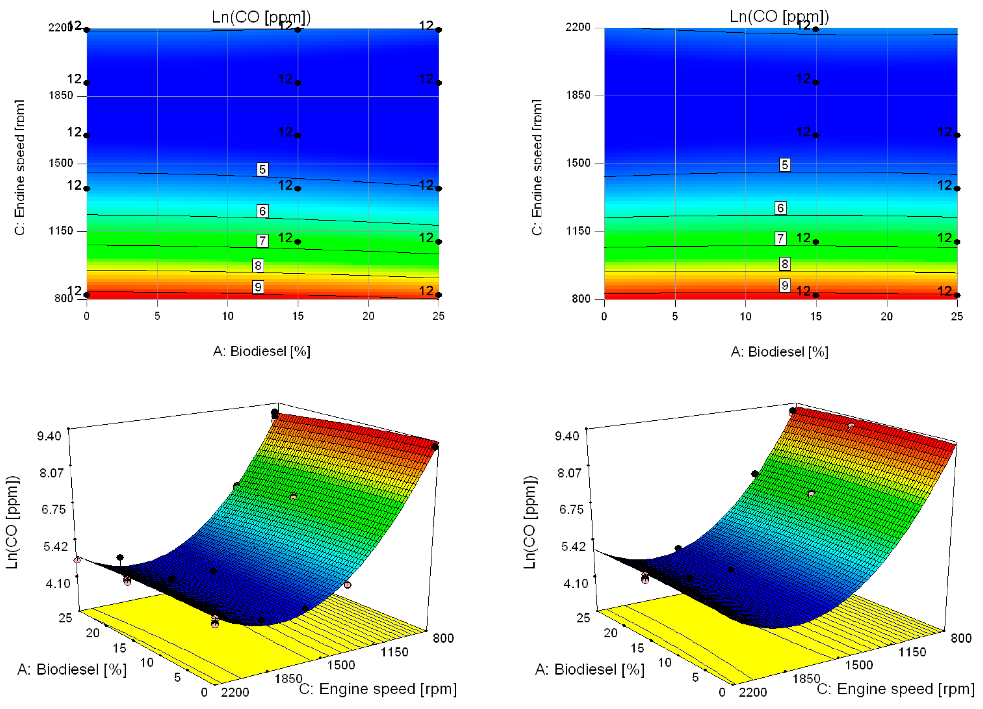
Figure 13.
Contour plots (top) and 3D-graphs (bottom) of the CO concentration as a function of the biodiesel percentage and of the engine speed referred to the 1st model (24 cases), with the 0% (left) and the 3% (right) of bioethanol in the blend (NB: the values of CO are reported as labels directly on the contours). The same pictures show also the positions of the experimental measurements (black dots positioned within the investigated hyperspace; notice that many points are positioned under the represented surface and hence are not visible).
Figure 14.
Contour plots (top) and 3D-graphs (bottom) of the CO concentration as a function of the biodiesel percentage and of the engine speed referred to the 2nd model (30 cases), with the 0% (left) and the 3% (right) of bioethanol in the blend (NB: the values of CO are reported as labels directly on the contours). The same pictures show also the positions of the experimental measurements (black dots positioned within the investigated hyperspace; notice that many points are positioned under the represented surface and hence are not visible).
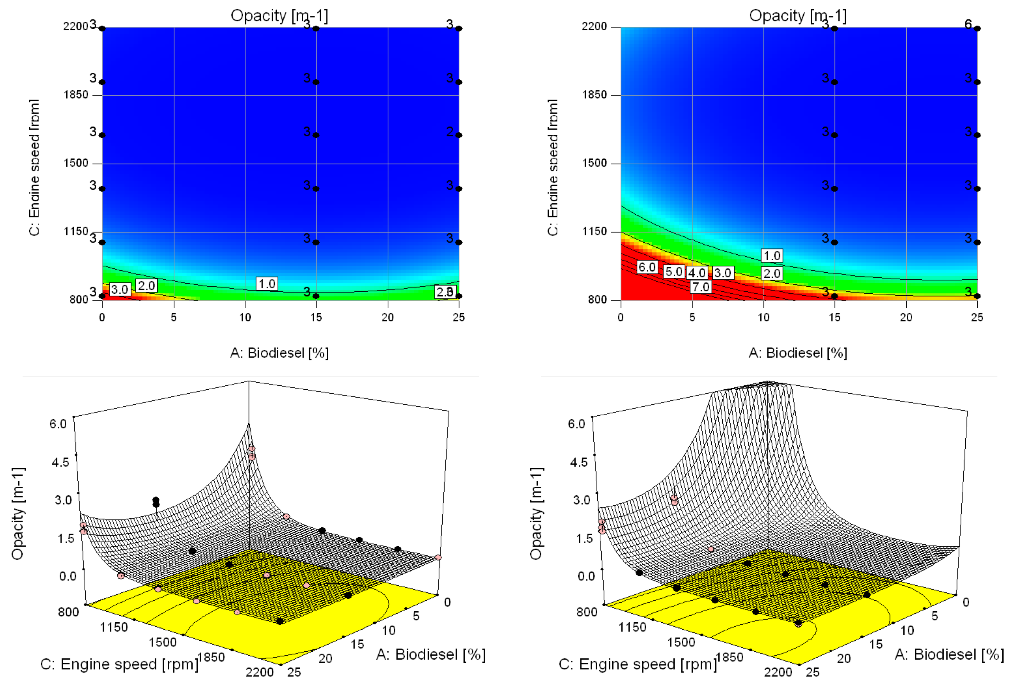
Figure 15.
Contour plots (top) and 3D-graphs (bottom) of the logarithm of the opacity of the exhaust gases as a function of the biodiesel percentage and of the engine speed referred to the 1st model (24 cases), with the 0% (left) and the 3% (right) of bioethanol in the blend (NB: the values of the logarithm of the opacity are reported as labels directly on the contours). The same pictures show also the positions of the experimental measurements (black dots positioned within the investigated hyperspace; notice that many points are positioned under the represented surface and hence are not visible).
Figure 16.
Contour plots (top) and 3D-graphs (bottom) of the logarithm of the exhaust gas opacity as a function of the biodiesel percentage and of the engine speed referred to the 2nd model (30 cases), with the 0% (left) and the 3% (right) of bioethanol in the blend (NB: the values of the logarithm of the opacity are reported as labels directly on the contours). The same pictures show also the positions of the experimental measurements (black dots positioned within the investigated hyperspace; notice that many points are positioned under the represented surface and hence are not visible).
Figure 17.
Contour plots (top) and 3D-graphs (bottom) of the exhaust gas opacity as a function of the biodiesel percentage and of the engine speed referred to the 2nd model (30 cases), with the 0% (left) and the 3% (right) of bioethanol in the blend (NB: the values of opacity are reported as labels directly on the contours). The same pictures show also the positions of the experimental measurements (black dots positioned within the investigated hyperspace; notice that many points are positioned under the represented surface and hence are not visible).
Figure 18.
Contour plot (left) and 3D-graph (right) of the engine torque as a function of fuel kinematic viscosity and of the engine speed referred to the 1st model (24 cases) (NB: the values of torque are reported as labels directly on the contours). The same pictures show also the positions of the experimental measurements (black dots positioned within the investigated hyperspace; notice that many points are positioned under the represented surface and hence are not visible).
Figure 19.
Contour plot (left) and 3D-graph (right) of the engine torque as a function of fuel kinematic viscosity and of the engine speed referred to the 2nd model (30 cases) (NB: the values of Table. are reported as labels directly on the contours). The same pictures show also the positions of the experimental measurements (black dots positioned within the investigated hyperspace; notice that many points are positioned under the represented surface and hence are not visible).
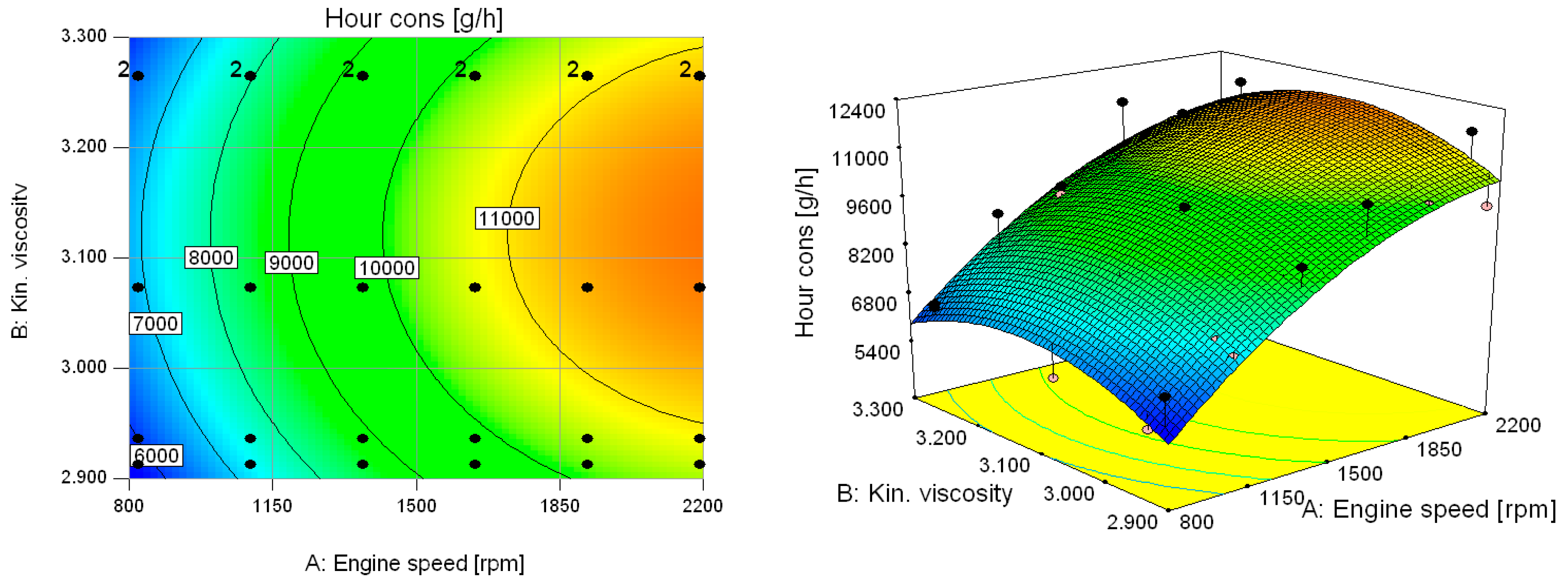
Figure 20.
Contour plot (left) and 3D-graph (right) of the hourly fuel consumption at full load as a function of fuel kinematic viscosity and of the engine speed referred to the 1st model (24 cases) (NB: the values of hourly fuel consumption are reported as labels directly on the contours). The same pictures show also the positions of the experimental measurements (black dots positioned within the investigated hyperspace; notice that many points are positioned under the represented surface and hence are not visible).
Figure 21.
Contour plot (left) and 3D-graph (right) of the hourly fuel consumption at full load as a function of fuel kinematic viscosity and of the engine speed referred to the 2nd model (30 cases) (NB: the values of hourly fuel consumption are reported as labels directly on the contours). The same pictures show also the positions of the experimental measurements (black dots positioned within the investigated hyperspace; notice that many points are positioned under the represented surface and hence are not visible).
Figure 22.
Contour plot (left) and 3D-graph (right) of the NOx concentration in the exhaust gases as a function of fuel kinematic viscosity and of the engine speed referred to the 1st model (24 cases) (NB: the values of NOx concentration are reported as labels directly on the contours). The same pictures show also the positions of the experimental measurements (black dots positioned within the investigated hyperspace; notice that many points are positioned under the represented surface and hence are not visible).
Figure 23.
Contour plot (left) and 3D-graph (right) of the NOx concentration in the exhaust gases as a function of fuel kinematic viscosity and of the engine speed referred to the 2nd model (30 cases) (NB: the values of NOx concentration are reported as labels directly on the contours). The same pictures show also the positions of the experimental measurements (black dots positioned within the investigated hyperspace; notice that many points are positioned under the represented surface and hence are not visible).
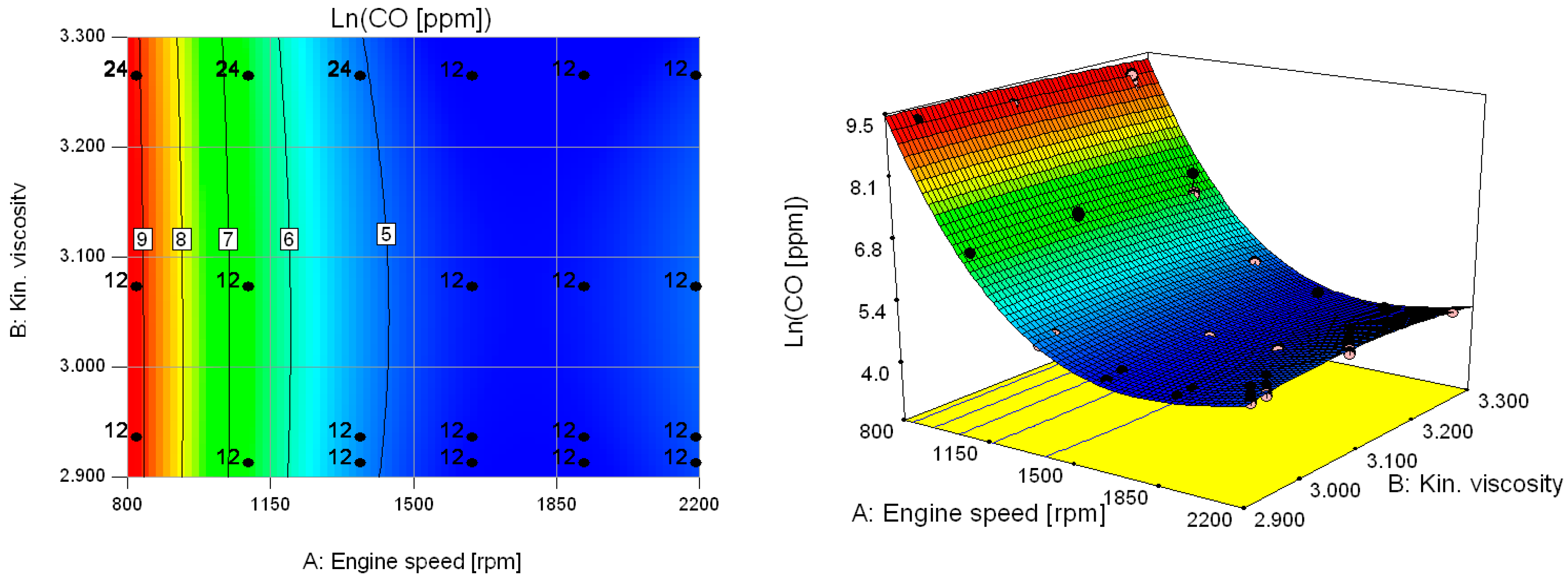
Figure 24.
Contour plot (left) and 3D-graph (right) of the logarithm of the CO concentration in the exhaust gases as a function of fuel kinematic viscosity and of the engine speed referred to the 1st model (24 cases) (NB: the values of the logarithm of CO concentration are reported as labels directly on the contours). The same pictures show also the positions of the experimental measurements (black dots positioned within the investigated hyperspace; notice that many points are positioned under the represented surface and hence are not visible).
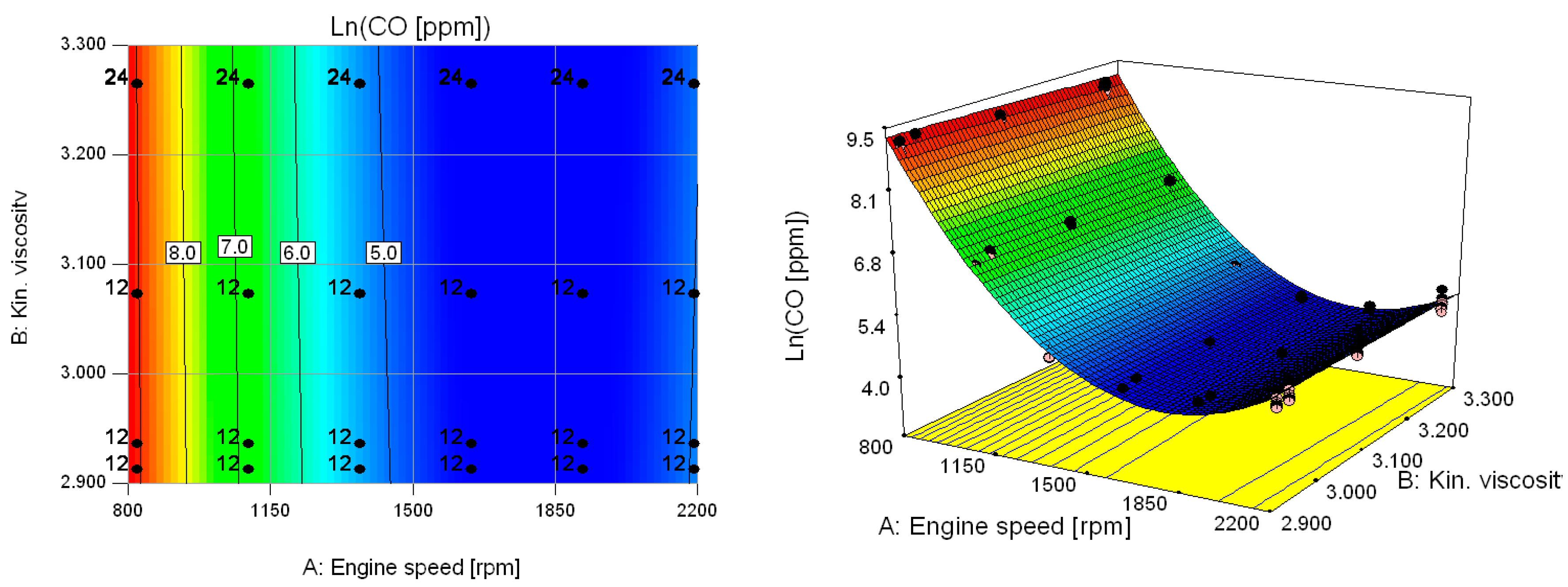
Figure 25.
Contour plot (left) and 3D-graph (right) of the logarithm of the CO concentration as a function of fuel kinematic viscosity and of the engine speed referred to the 2nd model (30 cases) (NB: the values of the logarithm of the CO concentration are reported as labels directly on the contours). The same pictures show also the positions of the experimental measurements (black dots positioned within the investigated hyperspace; notice that many points are positioned under the represented surface and hence are not visible).
Figure 26.
Contour plot (left) and 3D-graph (right) of the logarithm of the opacity (top) and of the opacity (bottom) of the exhaust gases as a function of fuel kinematic viscosity and of the engine speed referred to the 1st model (24 cases) (NB: the values of the logarithm of the opacity are reported as labels directly on the contours). The same pictures show also the positions of the experimental measurements (black dots positioned within the investigated hyperspace; notice that many points are positioned under the represented surface and hence are not visible).
Figure 27.
Contour plot (left) and 3D-graph (right) of the logarithm of the opacity (top) and of the opacity (bottom) as a function of fuel kinematic viscosity and of the engine speed referred to the 2nd model (30 cases) (NB: the values of the logarithm of the opacity are reported as labels directly on the contours). The same pictures show also the positions of the experimental measurements (black dots positioned within the investigated hyperspace; notice that many points are positioned under the represented surface and hence are not visible).
Table 1.
Diesel oil/biodiesel/bioethanol main physical and chemical properties and typical values [
4,
12,
13].
Table 1.
Diesel oil/biodiesel/bioethanol main physical and chemical properties and typical values [
4,
12,
13].
| Fuel Property | Measurement Unit | Value |
|---|
| Diesel Oil | Biodiesel | Bioethanol |
|---|
| Cetane number | - | 52 | 51 | 6 |
| Lower heating value | MJ kg−1 | 42.5 | 37.5 | 28.4 |
| Density @ 20 °C | kg m−3 | 840 | 871 | 786 |
| Viscosity @ 40 °C | mPa s | 2.4 | 4.6 | 1.2 |
| Latent heat of evaporation | kJ kg−1 | 250–290 | 300 | 840 |
| Carbon content | % (on mass) | 86.6 | 77.1 | 52.5 |
| Hydrogen content | % (on mass) | 13.4 | 12.1 | 13.0 |
| Oxygen content | % (on mass) | 0.0 | 10.8 | 34.8 |
| Sulphur content | mg kg−1 | 10–30 | <10 | - |
| Boiling point | °C | 210–235 | 300–350 | 79 |
| Flash point | °C | 52–96 | 120–170 | 12 |
Table 2.
Main properties of the New Holland T4020V farm tractor.
Table 2.
Main properties of the New Holland T4020V farm tractor.
| Description | Specification |
|---|
| Engine (manufacturer; type; building year; total displacement) | New Holland; F5A E9484A*A001; 2009; 3200 cm3 |
| Cylinders (number; configuration) | 4; straight |
| Fuel-system type (features and accessories) | With: direct injection, rotary fuel-pump, turbocharger, intercooler, mechanical speed-regulator |
| Nominal gross power at the engine (value, engine speed) | 47.7 kW (according to ISO/TR 14396:1996) @ 2300 rpm |
| Maximum torque (value; engine speed) | 290 Nm @ 1250 rpm |
Table 3.
Main properties of the diesel oil, the biodiesel and the bioethanol used in the tests.
Table 3.
Main properties of the diesel oil, the biodiesel and the bioethanol used in the tests.
| Fuel | Property | Value | Unit | Test Method |
|---|
| Diesel oil | Density at 15 °C | 820.0–845.0 | kg m−3 | EN ISO 12185
EN ISO 3675 |
| Viscosity at 40 °C | 2.0–4.5 | mm2 s−1 | EN ISO 3104 |
| Flash point | >55 | °C | EN ISO 2719 |
| Cetane number | >51 | - | EN ISO 5165
EN 15195
EN 1614 |
| Copper strip corrosion (3 h at 50 °C) | Class 1 | - | EN ISO 2160 |
| Lubricity, correct wear scar | 460 | μm | EN ISO 12156 |
| Biodiesel | Density at 15 °C | 883.1 | kg m−3 | EN ISO 3675 |
| Viscosity at 40 °C | 4.1–4.7 | mm2 s−1 | EN ISO 3104 |
| Flash point | >160 | °C | EN ISO 3679 |
| Cetane number | >51 | - | EN ISO 5165 |
| Water content | 210 | mg kg−1 | EN ISO 12937 |
| Ester content | 98.5 | % (on mass) | EN 14103 |
| Bioethanol | Ethanol content | 99.3 | % (on mass) | EN 15721 |
| Water content | 0.150 | % (on mass) | EN ISO 15489 |
| Total acidity (expressed as acetic acid) | 0.001 | % (on mass) | EN ISO 15491 |
| Electrical conductivity | 0.45 | µS cm−1 | EN ISO 15938 |
| Sulphur content | 0.3 | mg kg−1 | EN ISO 15486 |
| pH | 8.6 | - | EN 15490 |
Table 4.
Kinematic viscosity of the used fuel blends.
Table 4.
Kinematic viscosity of the used fuel blends.
| Denomination of the Fuel/Blend | D (%) | B (%) | E (%) | Kinematic Viscosity at 40 °C (mm2 s−1) |
|---|
| Mean Value | Std. dev. |
|---|
| D100* | 100 | 0 | 0 | 2.936 | 0.148 |
| B15 | 85 | 15 | 0 | 2.912 | 0.062 |
| B25 | 75 | 25 | 0 | 3.265 | 0.131 |
| B15E3 | 82 | 15 | 3 | 3.073 | 0.129 |
| B25E3 | 75 | 25 | 3 | 3.264 | 0.270 |
Table 5.
Main data concerning the two numerical models (respectively based on 24 and 30 cases) and the predictions of the models in six selected cases for the engine torque.
Table 5.
Main data concerning the two numerical models (respectively based on 24 and 30 cases) and the predictions of the models in six selected cases for the engine torque.
| Quantity | Model |
|---|
| nr. 1 (on 24 cases) | nr. 2 (on 30 cases) |
|---|
| Regression equation | T [Nm] = +749.85629 + 0.86775 ∙ B [%] −5.46458 ∙ E [%] + 8.48014 ∙ 10−3 ∙ n [rpm] −6.15737 ∙ 10−5 ∙ {n [rpm]}2 | T [Nm] = +751.73874+0.77198 ∙ B [%]−5.63968 ∙ E [%] + 9.55847 ∙ 10−3 ∙ n [rpm]−6.24263 ∙ 10−5 ∙ {n[rpm]}2 |
| Fitting (on available cases) | R2 | 0.9918 | 0.9930 (+0.0012) |
| Adj. R2 | 0.9901 | 0.9918 (+0.0017) |
| Ave. error | 0.07% | 0.00% (−0.07%) |
| Mean sq. er. | 0.01% | 0.01% (+0.00%) |
| Prediction (on 6 cases) | Ave. error | 0.38% | - |
| Mean sq. er. | 0.01% | - |
Table 6.
Main data concerning the two numerical models (respectively based on 24 and 30 cases) and the predictions of the models in six selected cases for the hourly fuel consumption at full load.
Table 6.
Main data concerning the two numerical models (respectively based on 24 and 30 cases) and the predictions of the models in six selected cases for the hourly fuel consumption at full load.
| Quantity | Model |
|---|
| nr. 1 (on 24 cases) | nr. 2 (on 30 cases) |
|---|
| Regression equation | ch[g h−1] = −561.22973 +73.05882 ∙ B[%]−725.37929 ∙ E[%] +8.73898 ∙ n[rpm] +14.39175 ∙ B[%] ∙ E[%]−0.041545 ∙ B[%] ∙ n[rpm] +0.56033 ∙ E[%] ∙ n[rpm] −1.59042 ∙ 10−3 ∙ {n[rpm]}2 | ch[g h−1] = −1531.53212 +96.13334 ∙ B[%]−229.40642 ∙ E[%] +10.17610 ∙ n[rpm] −0.061286 ∙ B[%] ∙ n[rpm] +0.36366 ∙ E[%] ∙ n[rpm] −2.02194 ∙ 10−3 ∙{ n[rpm]}2 |
| Fitting (on available cases) | R2 | 0.9248 | 0.9040 (−0.0208) |
| Adj. R2 | 0.8918 | 0.8790 (−0.0128) |
| Ave. error | 0.50% | 0.00% (−0.50%) |
| Mean sq. er. | 0.41% | 0.35% (−0.06%) |
| Prediction (on 6 cases) | Ave. error | 2.48% | - |
| Mean sq. er. | 0.92% | - |
Table 7.
Main data concerning the two numerical models (respectively based on 24 and 30 cases) and the predictions of the models in six selected cases for the NOx concentration in the exhaust gases.
Table 7.
Main data concerning the two numerical models (respectively based on 24 and 30 cases) and the predictions of the models in six selected cases for the NOx concentration in the exhaust gases.
| Quantity | Model |
|---|
| nr. 1 (on 24 cases) | nr. 2 (on 30 cases) |
|---|
| Regression equation | NOx[ppm] = +500.71510 −0.61435 ∙ B[%] +25.06639 ∙ E[%] +0.13109 ∙ n[rpm] −1.77110 ∙ B[%] ∙ E[%]−4.43123 ∙ 10−4 ∙ B[%] ∙ n[rpm] −3.82978 ∙ 10−3 ∙ E[%] ∙ n[rpm] +0.21606 ∙ {B[%]}2 −1.25658 ∙ 10−4 ∙ {n[rpm]}2 | NOx[ppm] = +488.75020 −0.37219 ∙ B[%] +25.65112 ∙ E[%] +0.14445 ∙ n[rpm] −1.81991 ∙ B[%] ∙ E[%]−5.89491 ∙ 10−4 ∙ B[%] ∙ n[rpm] −4.67969 ∙ 10−3 ∙ E[%] ∙ n[rpm] +0.22224 ∙ {B[%]}2 −1.29296 ∙ 10−4 ∙ {n[rpm]}2 |
| Fitting (on available cases) | R2 | 0.9825 | 0.9820 (−0.0005) |
| Adj. R2 | 0.9820 | 0.9816 (−0.0004) |
| Ave. error | 0.36% | 0.11% (−0.25%) |
| Mean sq. er. | 0.17% | 0.15% (−0.02%) |
| Prediction (on 6 cases) | Ave. error | 1.40% | - |
| Mean sq. er. | 0.25% | - |
Table 8.
Main data concerning the two numerical models (respectively based on 24 and 30 cases) and the predictions of the models in six selected cases for the CO concentration in the exhaust gases.
Table 8.
Main data concerning the two numerical models (respectively based on 24 and 30 cases) and the predictions of the models in six selected cases for the CO concentration in the exhaust gases.
| Quantity | Model |
|---|
| nr. 1 (on 24 cases) | nr. 2 (on 30 cases) |
|---|
| Regression equation | Ln(CO[ppm]) = +20.34397 −9.60882 ∙ 10−3 ∙ B[%]−0.026016 ∙ E[%]−0.017564 ∙ n[rpm] +4.31472 ∙ 10−3 ∙ B[%] ∙ E[%] +5.77145 ∙ 10−6 ∙ B[%] ∙ n[rpm] −4.00363 ∙ 10−4 ∙ {B[%]}2 +4.82341 ∙ 10−6 ∙ {n[rpm]}2 | Ln(CO[ppm]) = +20.35606 −5.47853 ∙ 10−3 ∙ B[%]−0.077395 ∙ E[%]−0.017594 ∙ n[rpm] +5.69115 ∙ 10−3 ∙ B[%] ∙ E[%] +4.64820 ∙ 10−6 ∙ B[%] ∙ n[rpm] −4.26751 ∙ 10−4 ∙ {B[%]}2 +4.83437 ∙ 10−6 ∙ {n[rpm]}2 |
| Fitting (on available cases) | R2 | 0.9879 | 0.9869 (+0.001) |
| Adj. R2 | 0.9876 | 0.9866 (+0.001) |
| Ave. error | −1.46% | −1.84% (+0.38%) |
| Mean sq. er. | 3.32% | 3.18% (+0.14%) |
| Prediction (on 6 cases) | Ave. error | −0.91% | - |
| Mean sq. er. | 4.47% | - |
Table 9.
Main data concerning the two numerical models (respectively based on 24 and 30 cases) and the predictions of the models in six selected cases for the opacity of the exhaust gases.
Table 9.
Main data concerning the two numerical models (respectively based on 24 and 30 cases) and the predictions of the models in six selected cases for the opacity of the exhaust gases.
| Quantity | Model |
|---|
| nr. 1 (on 24 cases) | nr. 2 (on 30 cases) |
|---|
| Regression equation | Ln(Opacity[m−1]) = +11.84735 −0.21196 ∙ B[%] +0.60734 ∙ E[%]−0.016407 ∙ n[rpm] −0.020619 ∙ B[%] ∙ E[%] +2.41216 ∙ 10−5 ∙ B[%] ∙ n[rpm] +6.11103 ∙ 10−3 ∙ {B[%]}2 +4.50634 ∙ 10−6 ∙ {n[rpm]}2 | Ln(Opacity [m−1]) =+11.44037 −0.14504 ∙ B[%] +0.61544 ∙ E[%]−0.016037 ∙ n[rpm] −0.023313 ∙ B[%] ∙ E[%] +4.80098 ∙ 10−3 ∙ {B[%]}2 +4.43092 ∙ 10−6 ∙ {n[rpm]}2 |
| Fitting (on available cases) | R2 | 0.9242 | 0.8993 (−0.0249) |
| Adj. R2 | 0.9159 | 0.8922 (−0.0237) |
| Ave. error | −5.60% | −9.48% (−3.88%) |
| Mean sq. er. | 18.21% | 22.04% (+3.83%) |
| Prediction (on 6 cases) | Ave. error | 5.62% | - |
| Mean sq. er. | 40.07% | - |
Table 10.
Main data concerning the two numerical models (respectively based on 24 and 30 cases) and the predictions of the models in six selected cases for the engine torque.
Table 10.
Main data concerning the two numerical models (respectively based on 24 and 30 cases) and the predictions of the models in six selected cases for the engine torque.
| Quantity | Model |
|---|
| nr. 1 (on 24 cases) | nr. 2 (on 30 cases) |
|---|
| Regression equation | T[Nm] = +713.67423 +7.20838 ∙ 10−3 ∙ n[rpm] +14.32782 ∙ ν[mm2 s−1] −6.14489 ∙ 10−5 ∙ {n[rpm]}2 | T[Nm] = +5025.45458 +9.55847 ∙ 10−3 ∙ n[rpm] −2773.64811 ∙ ν[mm2 s-1] −6.24263 ∙ 10−5 ∙ {n[rpm]}2 +449.51032 ∙ {ν[mm2 s−1]}2 |
| Fitting (on available cases) | R2 | 0.9806 | 0.9865 (+0.0059) |
| Adj. R2 | 0.9776 | 0.9843 (+0.0067) |
| Ave. error | −0.08% | 0.00% (+0.08%) |
| Mean sq. er. | 0.03% | 0.03% (+0.00%) |
| Prediction (on 6 cases) | Ave. error | 0.40% | - |
| Mean sq. er. | 0.02% | - |
Table 11.
Main data concerning the two numerical models (respectively based on 24 and 30 cases) and the predictions of the models in six selected cases for the hourly fuel consumption at full load.
Table 11.
Main data concerning the two numerical models (respectively based on 24 and 30 cases) and the predictions of the models in six selected cases for the hourly fuel consumption at full load.
| Quantity | Model |
|---|
| nr. 1 (on 24 cases) | nr. 2 (on 30 cases) |
|---|
| Regression equation | ch[g h−1] = −2.74704 ∙ 10+5 +10.79205 ∙ n[rpm] +1.74994 ∙ 10+5 ∙ ν[mm2 s−1] −2.32805 ∙ 10−3 ∙ {n[rpm]}2 −27922.84094 ∙ {ν[mm2 s−1]}2 | ch[g h−1] = −2.71164 ∙ 10+5 +9.63191 ∙ n[rpm] +1.74045 ∙ 10+5 ∙ ν[mm2 s−1] −2.02194 ∙ 10−3 ∙ {n[rpm]}2 −27885.68040 ∙ {ν[mm2 s−1]}2 |
| Fitting (on available cases) | R2 | 0.8608 | 0.8571 (−0.0037) |
| Adj. R2 | 0.8314 | 0.8343 (+0.0029) |
| Ave. error | −0.18% | −0.06% (+0.12%) |
| Mean sq. er. | 0.66% | 0.60% (−0.06%) |
| Prediction (on 6 cases) | Ave. error | −0.86% | - |
| Mean sq. er. | 1.05% | - |
Table 12.
Main data concerning the two numerical models (respectively based on 24 and 30 cases) and the predictions of the models in six selected cases for the NOx.
Table 12.
Main data concerning the two numerical models (respectively based on 24 and 30 cases) and the predictions of the models in six selected cases for the NOx.
| Quantity | Model |
|---|
| nr. 1 (on 24 cases) | nr. 2 (on 30 cases) |
|---|
| Regression equation | NOx[ppm] = +13839.40181 −0.20309 ∙ n[rpm] −8624.79484 ∙ ν[mm2 s−1] +0.084559 ∙ n[rpm] ∙ ν[mm2 s−1] −1.02166 ∙ 10−4 ∙ {n[rpm]}2 +1400.09439 ∙ {ν[mm2 s−1]}2 | NOx[ppm] = +12680.14971 +0.12940 ∙ n[rpm] −8011.28620 ∙ ν[mm2 s−1] −1.29296 ∙ 10−4 ∙{n[rpm]}2 +1318.53010 ∙ {ν[mm2 s−1]}2 |
| Fitting (on available cases) | R2 | 0.9546 | 0.9397 (−0.0149) |
| Adj. R2 | 0.9538 | 0.9390 (−0.0148) |
| Ave. error | 1.65% | 0.08% (−1.57%) |
| Mean sq. er. | 0.81% | 0.68% (−0.13%) |
| Prediction (on 6 cases) | Ave. error | 7.56% | - |
| Mean sq. er. | 2.67% | - |
Table 13.
Main data concerning the two numerical models (respectively based on 24 and 30 cases) and the predictions of the models in six selected cases for the CO concentration in the exhaust gases.
Table 13.
Main data concerning the two numerical models (respectively based on 24 and 30 cases) and the predictions of the models in six selected cases for the CO concentration in the exhaust gases.
| Quantity | Model |
|---|
| nr. 1 (on 24 cases) | nr. 2 (on 30 cases) |
|---|
| Regression equation | Ln(CO[ppm]) = +42.88856 −0.063008 ∙ n[rpm] −10.69428 ∙ ν[mm2 s−1] +0.020956 ∙ n[rpm] ∙ ν[mm2 s−1] +1.41593 ∙ 10−5 ∙ {n[rpm]}2 +1.68731 ∙ {ν[mm2 s−1]}2 −3.39237 ∙ 10−3 ∙ n[rpm] ∙ {ν[mm2 s−1]}2−2.07463 ∙ 10−9 ∙ {n[rpm]}3 | Ln(CO[ppm]) = +21.01646 −0.017519 ∙ n[rpm] −0.27489 ∙ ν[mm2 s−1] +4.83437 ∙ 10−6 ∙ {n[rpm]}2 |
| Fitting (on available cases) | R2 | 0.9929 | 0.9851 (−0.0078) |
| Adj. R2 | 0.9928 | 0.9850 (−0.0078) |
| Ave. error | −1.91% | −1.96% (−0.05%) |
| Mean sq. er. | 2.02% | 3.52% (+1.50%) |
| Prediction (on 6 cases) | Ave. error | −5.34% | - |
| Mean sq. er. | 2.88% | - |
Table 14.
Main data concerning the two numerical models (respectively based on 24 and 30 cases) and the predictions of the models in six selected cases for the opacity in the exhaust gases.
Table 14.
Main data concerning the two numerical models (respectively based on 24 and 30 cases) and the predictions of the models in six selected cases for the opacity in the exhaust gases.
| Quantity | Model |
|---|
| nr. 1 (on 24 cases) | nr. 2 (on 30 cases) |
|---|
| Regression equation | Ln(Opacity [m−1]) = −92.08952 −0.024706 ∙ n[rpm] +70.29248 ∙ ν[mm2 s−1] +2.57254 ∙ 10−3 ∙ n[rpm] ∙ ν[mm2 s−1] +4.72809 ∙ 10−6 ∙ {n[rpm]}2 −11.88675 ∙ {ν[mm2 s−1]}2 | Ln(Opacity [m−1]) = −134.34316 −0.016059 ∙ n[rpm] +94.08222 ∙ ν[mm2 s−1] +4.44021 ∙ 10−6 ∙ {n[rpm]}2 −15.19390 ∙ {ν[mm2 s−1]}2 |
| Fitting (on available cases) | R2 | 0.8781 | 0.8616 (−0.0165) |
| Adj. R2 | 0.8689 | 0.8552 (−0.0137) |
| Ave. error | −7.14% | −13.17% (−6.03%) |
| Mean sq. er. | 25.90% | 31.15% (+5.25%) |
| Prediction (on 6 cases) | Ave. error | 18.95% | - |
| Mean sq. er. | 20.84% | - |
Table 15.
Main data concerning the numerical models of several quantities as a function of the fuel blend composition and of the engine speed.
Table 15.
Main data concerning the numerical models of several quantities as a function of the fuel blend composition and of the engine speed.
| Investigated Response | Model nr. | Regr. Eq. Order | Fitting (on available cases) | Prediction (on 6 cases) |
|---|
| R2 | Adj. R2 | Ave.Error | Mean sq. Error | Ave. Error | Mean sq. Error |
|---|
| Torque [Nm] | nr. 1 (on 24 cases) | 2 | 0.9918 | 0.9901 | 0.07% | 0.01% | 0.38% | 0.01% |
| nr. 2 (on 30 cases) | 2 | 0.9930 (+0.0012) | 0.9918 (+0.0017) | 0.00% (−0.07%) | 0.01% (+0.00%) | - | - |
| Hour cons [g h−1] | nr. 1 (on 24 cases) | 2 | 0.9248 | 0.8918 | 0.50% | 0.41% | 2.48% | 0.92% |
| nr. 2 (on 30 cases) | 2 | 0.9040 (−0.0208) | 0.8790 (−0.0128) | 0.00% (−0.50%) | 0.35% (−0.06%) | - | - |
| NOx [ppm] | nr. 1 (on 24 cases) | 2 | 0.9825 | 0.9820 | 0.36% | 0.17% | 1.40% | 0.25% |
| nr. 2 (on 30 cases) | 2 | 0.9820 (−0.0005) | 0.9816 (−0.0004) | 0.11% (−0.25%) | 0.15% (−0.02%) | - | - |
| Ln (CO [ppm]) | nr. 1 (on 24 cases) | 2 | 0.9879 | 0.9876 | −1.46% | 3.32% | −0.91% | 4.47% |
| nr. 2 (on 30 cases) | 2 | 0.9869 (+0.001) | 0.9866 (+0.001) | −1.84% (+0.38%) | 3.18% (+0.14%) | - | - |
| Ln (Opacity [m−1]) | nr. 1 (on 24 cases) | 2 | 0.9242 | 0.9159 | −5.60% | 18.21% | 5.62% | 40.07% |
| nr. 2 (on 30 cases) | 2 | 0.8993 (−0.0249) | 0.8922 (−0.0237) | −9.48% (−3.88%) | 22.04% (+3.83%) | - | - |
Table 16.
Main data concerning the numerical models of several quantities as a function of the fuel blend viscosity and of the engine speed.
Table 16.
Main data concerning the numerical models of several quantities as a function of the fuel blend viscosity and of the engine speed.
| Investigated Response | Model nr. | Regr. Eq. Order | Fitting (on available cases) | Prediction (on 6 cases) |
|---|
| R2 | Adj. R2 | Ave. Error | Mean sq. Error | Ave. Error | Mean sq. Error |
|---|
| Torque [Nm] | nr. 1 (on 24 cases) | 2 | 0.9806 | 0.9776 | −0.08% | 0.03% | 0.40% | 0.02% |
| nr. 2 (on 30 cases) | 2 | 0.9865 (+0.0059) | 0.9843 (+0.0067) | 0.00% (+0.08%) | 0.03% (+0.00%) | - | - |
| Hour cons [g h−1] | nr. 1 (on 24 cases) | 2 | 0.8608 | 0.8314 | −0.18% | 0.66% | −0.86% | 1.05% |
| nr. 2 (on 30 cases) | 2 | 0.8571 (−0.0037) | 0.8343 (+0.0029) | −0.06% (+0.12%) | 0.60% (−0.06%) | - | - |
| NOx [ppm] | nr. 1 (on 24 cases) | 2 | 0.9546 | 0.9538 | 1.65% | 0.81% | 7.56% | 2.67% |
| nr. 2 (on 30 cases) | 2 | 0.9397 (−0.0149) | 0.9390 (−0.0148) | 0.08% (−1.57%) | 0.68% (−0.13%) | - | - |
| Ln (CO [ppm]) | nr. 1 (on 24 cases) | 3 | 0.9929 | 0.9928 | −1.91% | 2.02% | −5.34% | 2.88% |
| nr. 2 (on 30 cases) | 2 | 0.9851 (−0.0078) | 0.9850 (−0.0078) | −1.96% (−0.05%) | 3.52% (+1.50%) | - | - |
| Ln (Opacity [m−1]) | nr. 1 (on 24 cases) | 2 | 0.8781 | 0.8689 | −7.14% | 25.90% | 18.95% | 20.84% |
| nr. 2 (on 30 cases) | 2 | 0.8616 (−0.0165) | 0.8552 (−0.0137) | −13.17% (−6.03%) | 31.15% (+5.25%) | - | - |
Table 17.
Positive (+), negative (-) or complex (x) correlations of each factor (column headings) with the indicated response (row headings); the investigated model is nr. 2 for each response.
Table 17.
Positive (+), negative (-) or complex (x) correlations of each factor (column headings) with the indicated response (row headings); the investigated model is nr. 2 for each response.
| Investigated Response | Engine outputs as a Function of the Composition of the Blends | Engine Outputs as a Function of the Viscosity of the Blends |
|---|
| Biodiesel [%] | Bioethanol [%] | Engine Speed [rpm] | Kin. Viscosity [mm2 s−1] | Engine Speed [rpm] |
|---|
| Torque [Nm] | + | - | - | x | - |
| Hour cons [g h−1] | x | + | + | x | + |
| NOx [ppm] | + | - | - | x | - |
| Ln (CO [ppm]) | - | + | - | - | x |
| Ln (Opacity [m−1]) | - | - | x | x | - |


