Practicalities and Driving Dynamics of a Real Driving Emissions (RDE) Euro 6 Regulation Homologation Test


Flow, Aerosols & Thermal Energy (FATE) Group, Deakin University, 75 Pigdons Rd, Victoria 3216, Australia
*
Author to whom correspondence should be addressed.
Energies 2019, 12(12), 2306; https://doi.org/10.3390/en12122306
Submission received: 23 May 2019
/
Revised: 13 June 2019
/
Accepted: 13 June 2019
/
Published: 17 June 2019
(This article belongs to the Special Issue Recent Technologies on Using Biofuels in I.C. Engines for Improved Combustion and Emissions Mitigation)
Abstract
:One of the most important sources of air pollution, especially in urban areas, is the exhaust emissions from passenger cars. New European emissions regulations, to minimize the gap between manufacturer-reported emissions and those emitted on the road, require new vehicles to undergo emission testing on public roads during the certification process. Outlined in the new regulation are specific boundary conditions to which the route on which the vehicle is driven must comply during a legal test. These boundary conditions, as they relate to the design and subsequent driving of a compliant route, are discussed in detail. The practicality of designing a compliant route is discussed in the context of developing a route on the Gold Coast in Queensland, Australia, in a prescriptive manner. The route itself was driven 5 times and the results compared against regulation boundary conditions.
1. Introduction
Air pollution, which is a significant environmental hazard, leads to serious diseases and therefore to high costs for health-care systems [1]. In 2018, the World Health Organisation (WHO) deemed that more than 95% of people in urban areas of Europe are exposed to unsafe concentrations of NO or particulate matter (PM) in the ambient air [1]. To improve ambient air quality, regulations on vehicle exhaust emissions have been progressively implemented by governments and authorities forcing the automotive industry to improve their products in terms of hazardous emissions [2], while simultaneously forcing the fuel market to improve the quality of fuel [3]. However, in reality, the emissions reduction forced by emissions standards were less effective than what was expected [2]. For example, NO emissions during an on-road emissions test have been frequently reported to be significantly higher than the measured emissions during a standard driving cycle (e.g., New European Driving Cycle (NEDC) and Worldwide Harmonized Light Duty Cycle (WLTC)) running on a chassis dynamometer in an emissions laboratory [4]. Additionally, many independently tested vehicles also exceed the emissions limits defined in the regulation for type approval tests [5,6,7,8,9]. Owing to the significant difference between the measured emissions during a homologation test in a laboratory compared to an on-road test, several national investigation programs such RDW [10] and GOV.UK [11] were launched to investigate.
Substantive differences between the emissions emitted by light duty vehicles during a homologation test on the NEDC and in practice on public roads has prompted the European Commission to enact a new regulation to close the gap between emissions reported by vehicle manufacturers and those actually emitted, especially in relation to NO (nitrogen oxide) emissions [12,13,14]. Apart from driver’s behavior and ambient conditions, this large discrepancy is a combination of two key effects, the cycle itself not being representative of real driving [15] and the load applied to the vehicle (the road load—a combination of rolling and aerodynamic resistance) not being representative of the vehicle under normal driving conditions [16,17,18]. The road load is typically determined from a coast-down test under artificially favorable conditions [19,20]. Increasing the road load and having potentially more demanding driving dynamics, compared to the NEDC test procedure, has the effect of moving the engine residency away from the low torque region to a higher torque region across a wider engine speed band. As vehicles have been specifically calibrated to comply to emissions levels on a particular test, they do not always perform well under off-cycle (the non-NEDC region of operation) conditions [21,22,23].
The NEDC consists of a phase representing urban driving (4 lots of the urban driving cycle ECE15) and a phase representing extra-urban driving (EUDC) [24], the cycle is shown in Figure 1. In terms of driving dynamics, an immediate issue with the NEDC cycle is that it is fixed on particular cruising speeds with no velocity transients and the accelerations are smooth and gentle. Therefore, the NEDC is not representative of real driving [15].
The WLTC, coupled to a new procedure for determining the road load and test procedure (WLTP), was introduced by the European Commission as a regulation driving cycle to overcome some of the limitations in the NEDC driving dynamics and test procedure [25,26]. These limitations include, but are not limited to, the soft acceleration and unrepresentative road loads.
In contrast to the NEDC, the WLTC speed profile was designed using real vehicle speed data. The cycle is shown in Figure 2. Diesel vehicles have been shown to be affected more than gasoline vehicles in the move from the NEDC to WLTC, with the increase in vehicle inertia and road loads being attributed as the key parameters for the increase, when compared to the NEDC [26].
There are also some other changes which made the WLTC more representative of real-world driving compared to the NEDC. For example, the drive trace during the NEDC had a significant tolerance, giving the driver the opportunity to cut corners, thereby driving less than the prescribed distance leading to lower fuel consumption and emissions. For example, Pavlovic et al. [27] studied the effect of driver behavior during NEDC by comparing different cycle parameters (such as speed and distance) from a standard NEDC and from an optimized NEDC in which the drive was within the tolerance. Results showed that the distance and average speed were 0.3 km and 0.9 km/h lower than the standard cycle. This has been improved in WLTC by normalizing the emissions according to the measured driven distance during the test [26,27]. Another change is through REESS (Rechargeable Electric Energy Storage System) monitoring which is called REESS charge balance (RCB) correction in which the CO emissions are required to be corrected according the amount of energy drawn from the battery during the test cycle [28,29]. This is owing to the fact that the vehicle battery is fully charged at the start of the test and it depletes during the cycle, which means the energy from the battery can be drawn and consumed over the cycle possibly leading to lower CO emissions and better fuel economy; however, this is not always the case in real driving conditions [28,29]. However, given time, any laboratory test cycle comes with the risk of exploitation by vehicle manufacturers.
The solution to minimize, or even eliminate, the discrepancy between homologation testing and real driving with respect to emissions has been to move part of the homologation requirement of new light duty vehicles from the laboratory to the public roads. This move with light duty vehicles has been possible owing to the introduction of light-weight accurate portable emissions measurement technology [21,30]. Portable emissions equipment has been in use with heavy-duty vehicle regulations for a decade [31]. Commission Regulation (EU) 2016/427 of 10 March 2016 an amendment of Regulation (EC) 692/2008 [14,32] is arguably the biggest change to emission rules for light duty vehicles since regulations of this sort were introduced and represents a significant challenge to vehicle manufacturers. Studies have shown, with particular emphasis on diesel vehicles, that regulations of this sort should reduce NO emissions [33] and therefore improve urban air quality. Certainly, in the wake of the VW scandal [34] stronger regulation is required to not only ensure compliance with the law but also to ensure continuing public trust in diesel technology [13].
Despite the obvious benefit and necessity of the move to homologate light duty vehicles on public roads, there are some great difficulties. From a practical perspective for vehicle manufacturers, this new regulation will substantially increase not only the calibration effort but also the emission testing and laboratory requirements during product development. From a calibration perspective, the substantial range of potential driving dynamics caused by differences between drivers and driving routes will increase the workload required to have a vehicle ready for homologation testing substantially. This is in addition to the significant effects of the environment and traffic. On the positive side of this coin, this will effectively stop the practice of cycle-beating to meet regulation requirements and therefore mean that manufacturers begin delivering vehicles that are more robust to a wider range of scenarios. From an emission testing perspective (for both development and homologation testing), the effort required to fit-out a vehicle with portable emissions equipment, travel to a suitable location for testing and then perform the tests are non-trivial. Moreover, the risks of having failed tests (in terms of boundary conditions from unforeseen circumstances, i.e., traffic causing an excess of urban driving) are also significant and could result in resource wastage.
Outside of these problems, which in essence can be dealt with by the allocation of additional personnel and resources, there is another significant issue with the practical side of the new regulation. Not all locations are able to accommodate a driving route which meets the boundary conditions set out in the regulation itself. There is a requirement, for example, to drive above 100 km/h for a minimum of 5 min during the motorway portion of the test. It would not be possible to meet this boundary condition unless there is a motorway proximal to the development site which has either a 110 km/h or greater speed limited road (in the United Kingdom, a 70 mph speed limited road would be required). The implication of this is that some vehicle manufacturers will not be able to easily test their vehicles during development from their usual development location. Having to develop vehicles in new locations will add a significant development cost to affected manufacturers, on top of the increased cost burden that on-road testing represents.
This paper will outline some of the key route design boundary conditions set out in the latest relevant Commission Regulation (EU) 2017/1154 of 7 June 2017 [35] and through the development and subsequent testing of a compliant route discuss the difficulties in developing a legal driving route. It is of note that, to date, the final RDE regulation is related to Package 4, Commission Regulation (EU) 2018/1832 of 5 November 2018 [36], in which there is no change compared to Package 3 in terms of boundary conditions and is mostly about in-service testing and market surveillance amendments. Hooftman et al. [2] reviewed the four RDE packages released to date explaining their differences.
A snap-shot understanding of where something was is always valuable; but it is equally, if not more, important to know where something is. For example, contrary to the earlier version of RDE regulation [14], the new amendment [35] proposed that the cold start period shall meet the same average speed requirements of the average urban driving, i.e., cold start average driving speed (including stops) should be between 15 and 40 km/h. This could mean that if a car manufacturer is exploiting the new rule, which allows driving on a road speed limited higher than 60 km/h at the start of a route, care would need to be taken to ensure that operation at near 60 km/h is not for too long. With the new amendment, the vehicle is also now not to be idle for greater than 90 s during the cold start period [35]. This would remove the option to force idle after a near 60 km/h cruise to lower the average vehicle speed during the cold start period.
While this study is intended to give an update of where the regulation is currently at, it should be keep in-mind that this is only going to be up-to-date at the time it was authored and may be superseded at the time it is being read. As such, it is recommended if you are using this work as a guide to develop your own driving route that you investigate the latest regulation for changes which may affect your route design.
It is envisaged that the discussion in this study could be used as a guide for the design of other RDE driving routes. Moreover, given that many vehicles are homologated for sale in Europe outside of Europe, including Australia, some discussion on the difficulties in meeting the driving boundary conditions on public roads outside of Europe is important. Appreciating here that the difficulties in this respect will vary between non-European, and even European, countries. Furthermore, for a complete picture, a discussion on the driving dynamics from multiple trips on the developed route will be given.
2. Selection of a Driving Route
2.1. Regulation
There are very specific rules about the route a vehicle is driven on during a homologation test. Table 1 shows the trip requirements of a valid RDE test according to the current regulation [36]. For example, it can be seen that the maximum cumulative positive altitude gain is 1200 m/100 km over the urban portion of the trip, in addition to the entire trip.
To have a valid drive the route should be designed such that the vehicle speed distribution is 29–44% urban driving, 23–43% rural driving and 23–43% motorway driving, by both topographical map and instantaneous speed, as shown in Table 1. Urban driving is classified as driving at 60 km/h or less, rural driving is driving between 60 and 90 km/h and motorway driving is driving above 90 km/h. In the case of the topographical map distribution, this is done using the speed limit for each road. It should be noted that it is not acceptable to simply drive at less than the speed limit for route design convenience, i.e., all urban driving must be done on roads with speed limits of 60 km/h or less and if there is a section of road during the urban driving in which the speed limit is higher than 60 km/h, the vehicle speed shall be operated up to 60 km/h [35]. Rural and motorway sections may contain roads with speed limits less than their classification—i.e., the rural section may be interrupted by some short periods of urban operation and the motorway section may be interrupted by some short periods of rural or urban operation [35]. The current regulation [35,36], states that in order to have a valid drive, the route must be designed such that by topographical map, the urban section is driven first followed by the rural and then the motorway sections. Given the cold start requirement, requiring a significant soak period, this is clearly problematic for locations not immediately attached to a road with a speed limit of 60 km/h or less.
There are other limiting rules associated with the design of a homologation route. The most limiting of these is that the vehicle must be driven above 100 km/h, as measured by the GPS, for at least 5 min. Also, detailed in the regulation is that the vehicle must adequately demonstrate driving between 90 and 110 km/h. Given that the displayed vehicle speed is greater than the vehicles true vehicle speed, see Figure 3, to be driving above 100 km/h, without asking the driver to exceed the speed limit, the vehicle must be driven on a road with a speed limit above 100 km/h—the maximum difference between the nominal and actual vehicle speeds shown in Figure 3 is 4.7 km/h and occurs at the fastest point, 110 km/h. This means that the route must contain a significant portion of the motorway section on a 110 km/h (or greater) speed limited road. In Australia, excluding some very remote locations, 110 km/h is the maximum speed limit which would be encountered on a speed limited road and for many locations there will not be a 110 km/h motorway proximal, this is similar for many European member states. In the United Kingdom, the maximum speed limit on a speed limited road is 70 mph (112 km/h). Therefore, to design a homologation route that meets the regulation criteria, the first step is to ensure that there is an accessible 110 km/h (or greater) motorway.
If it can be established that there exists an appropriate motorway section, the first step in designing a successful route is to find an appropriate rural section. For most countries engaging in on-road testing which meets the regulatory requirements, this means finding roads which are speed limited as 70, 80 or 90 km/h. However, in countries where the speed limits are in mph, such as the United Kingdom, to ensure success, the rural section needs to essentially be restricted to 50 mph roads—here, technically a 40 mph road meets the criteria, but this is only slightly above true 60 km/h and comes with a risk of obtaining too much instantaneous urban driving and hence a failed drive. The minimum distance for each of the urban, rural, and motorway sections are to be 16 km. However, the regulation is not specific about whether this minimum distance is by topographical map only or whether this minimum also needs to be met by the instantaneous speed. Moreover, the trip itself must take at least 90 min, but no more than 120 min. Anecdotally, if a route has a rural section of approximately 25 km by topographical map, it is likely to meet the time boundary condition and is unlikely to have instantaneous distances traveled less than 16 km in any of the sections. However, finding 25 km of continuous rural driving, without entering any road with a limit of 100 km/h or above, and limiting driving on roads with a speed limit of 60 km/h or less is not trivial. Especially when coupled to the requirement that this section will need to attach to the urban section of the start location and end at a suitable motorway. Please note that the rural section can, and often will need to, loop back upon itself (i.e., repeat roads) and therefore continuous rural driving here should not be taken to only mean a single 25 km stretch of rural road. It is also strongly recommended to avoid designing a rural section through urban areas, traffic and traffic lights will cause significant driving below 60 km/h and therefore come with a risk of exceeding the maximum of 44% instantaneous urban driving.
Assuming that the start location has a direct entry point into an urban area, there is an appropriate motorway and it was possible to find sufficient continuous rural driving, the remainder of the route design is reasonably trivial. The route should be designed in such a way as to protect against changes in future regulations, which have in the past switched between the end distribution being met by either or both of the topographical map or the instantaneous speed. This is achieved by designing the route to have the minimum urban distribution (–) and the maximum motorway distribution (–) by topographical map. Given that the motorway distance is difficult to alter, it is easiest, once a rural section has been mapped, to determine the motorway section next. An approximate urban distance can then easily be determined:
where u is the urban distance, r is the rural distance and m is the motorway distance, all by topographical map. Equation (1) assumes an urban topographical map share of 30%.
There are two related requirements that need consideration during the design of the urban section. Firstly, the average urban driving speed should be between 15 and 40 km/h. The low maximum upper-limit here is potentially problematic—it is possible to have a complete drive with an average urban speed above 40 km/h if the designed urban section is in some local streets with no traffic. Secondly, stop periods should account for 6–30% of the time duration of urban operation. A stop period is defined as when the vehicle speed is less than 1 km/h. Average stop periods in normal driving account for 8% ± 3% [21] and therefore represent a risk if it is not considered in the route design as it can become less than 6% and invalidate the drive. Additionally, the trip should contain several stop periods greater than 10 s. It is important to ensure that the urban section contains many opportunities for the vehicle to stop. This not only creates stop periods, but also acts to reduce the average urban driving speed.
Clear is that the regulation is aiming to mimic urban driving in a dense area. However, driving in a dense area can be problematic as the traffic may be too unpredictable, causing drives that exceed the maximum time, and dense urban areas are unlikely to have free-flowing rural roads adjacent to them, which could cause excessive urban operation during the rural section, thereby exceeding the maximum instantaneous urban driving share. A solution is to avoid using overly dense areas and rather instruct the driver to naturally pause the vehicle during the drive itself (for example at right-hand turns or intersections). While this may be counter to the intention of the regulation, it is not forbidden by it and therefore could be considered a sensible approach to designing a route. The regulation does, however, explicitly forbid using a single excessively long stop period (300 consecutive seconds).
Although not in the regulation, another consideration during the design of a route is the avoidance of speed bumps. In some cases, speed bumps have the potential to disturb the emission equipment and the potential to damage the connection to the exhaust pipe. Therefore, it is prudent to avoid them where possible; in some areas, this can be very problematic or impossible and care by the driver would need to be taken.
2.2. Test Route
For practical reasons, the test route designed in this study will have the start and end location at an Australian university—this will allow future use of the route by the authors for studies with emission equipment. Identified as a suitable location was Griffith University on the Gold Coast. Griffith University is located adjacent to a motorway (Smith St Motorway, which also attaches to a 110 km/h motorway, the Pacific Motorway) and an urban section (the suburbs of Parkwood and Arundel). Moreover, there are two potential rural driving sections connecting the suburbs back to the main motorway, the Pacific Motorway.
As discussed in Section 2.1, when designing a test route, once it has been established that a suitable motorway exists, it is generally advisable to identify the rural section. Initially a rural section was identified that began on Brisbane Rd, Arundel, then traveled along Olsen Ave through Labrador then continued through Ashmore, the rural section then continued south through Carrara and Robina ultimately ending at the Pacific Motorway. This potential section was abandoned owing to concerns related to traffic, the risk was too great that if any substantial traffic was encountered that too much driving would occur sub-60 km/h and produce a fail drive. Owing to the difficulty that can occur finding a suitable rural route, the temptation to use more urban-style roads with higher speed limits should be limited where possible. Traffic, traffic lights and roundabouts cause driving below 60 km/h. They can also cause driving behavior which would be classified as aggressive—which may become problematic when analyzing the emissions data, there are boundary conditions associated with driving style (a discussion on those is outside of the scope of this paper). It was identified that a more suitable rural section existed by initially going inland. Again, starting at Brisbane Rd in Arundel, the rural section travels west toward the Pacific Motorway and Helensvale. Continuing west on Brisbane Rd to Binstead Way into Maudsland, to travel south on Maudsland Rd into Mount Nathan on Mount Nathan Rd then Beaudesert Nerang Rd to eventually end the rural section at the Pacific Motorway at Nerang. This road had only limited driving in an urban area and very few roundabouts and traffic lights. The rural section is continuous rural driving for 25.1 km/h by topographical map and is shown in Figure 4. In this case, a single stretch of rural driving has been used as it was possible to do so (this was part of the motivation to perform this study in this area); however, it would have also have been possible to use just a segment of this and drive the rural portion in a loop.
If we assume that the urban section should also be approximately 25 km and that the motorway section should compromise of approximately 42% of the total distance by topographical map, to maximize motorway driving, then an estimate of the distance the motorway by topographical map should be is easily determined as:
This is achieved by first traveling south on the Pacific Motorway to the Pappas Way exit in North Nerang, turning around to travel north on the Pacific Motorway to the Dreamworld exit at Coomera, traveling onto Foxwell Rd (an urban speed limited road) to reconnect with the Pacific Motorway heading south again to eventually travel on the Smith St Motorway, which returns to the start location of Griffith University. This motorway section is ideal because the Pacific Motorway component is predominately speed limited as 110 km/h (ensuring at least 5 min of driving above 100 km/h) and the Smith St Motorway is 100 km/h speed limited (also ensuring that when driven, the route will allow a range of driving between 90 and 110 km/h to be demonstrated). The motorway section is 37.1 km long and is shown in Figure 5.
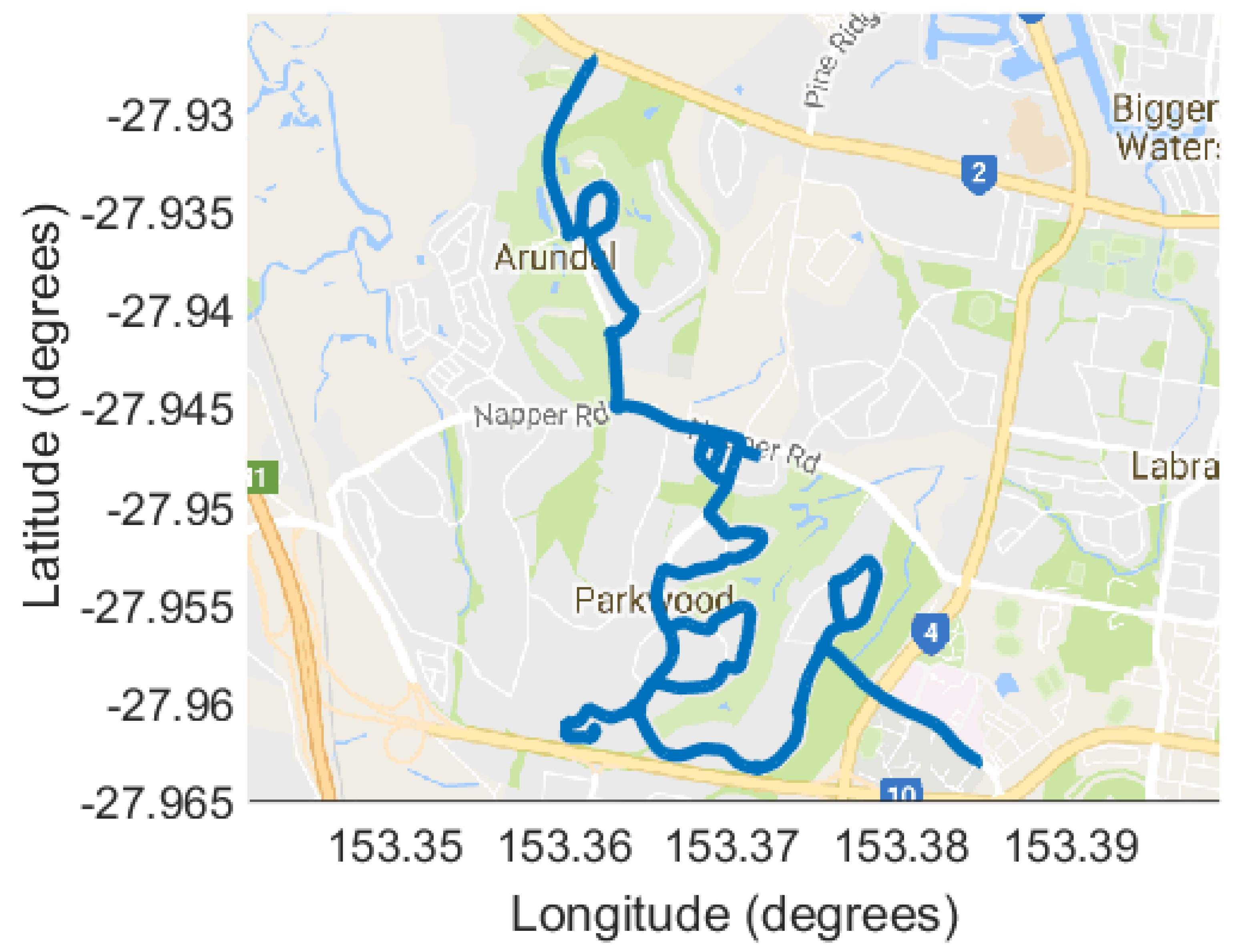
The target urban distance can now be calculated using Equation (1)—here the target urban distance is 26.6 km. Urban driving is achieved by looping through Parkwood and Arundel, suburbs adjacent to each other, Griffith University and the start of the rural section. Care was taken to ensure that there were many opportunities to stop the vehicle in natural driving, i.e., intersections and right-hand turns. The target distance was achieved, and the urban section is 26.6 km long, the streets the route is on are shown in Figure 6.
This route is a total of 88.8 km long and is estimated to take 1 h and 52 min (by Google Maps) to complete. By topographical map, the route comprises approximately 30.0%, 28.3% and 41.8% of urban, rural, and motorway driving, respectively.
Given that urban and motorway driving, by topographical map, have been minimized and maximized, respectively, it can be assumed that the route is likely to also meet the instantaneous distribution requirements. The route also meets all the criteria discussed in Section 2.1. Additionally, the test area is relatively flat, estimates using Google Maps indicate that the total positive change in elevation should be approximately 500 m/100 km across the route. Therefore, this route meets all the design criteria given in the latest regulation [36].
3. Experimental Setup
Keeping in line with the regulation requirement that says that the vehicle speed must be collected from GPS, rather than the vehicle, the data collection in this work was done using GPS. A GlobalSat G-STAR IV GPS Receiver was used with a Raspberry Pi device to log the data. The calculation requirements for reporting after a homologation test are done with 1 Hz data; therefore, the data for this study were logged at 1 Hz.
An automatic car was also selected in an attempt to minimize the effects of individual driving style on the output data. Although clearly the end dynamics are very driver dependent and can vary significantly between drivers. Moreover, differences in pedal maps, gearing, and vehicle power will also significantly influence the driving dynamics. It is assumed, however, that most people’s ‘normal’ driving will have a lot of similarities and certainly differences in rural and motorway driving, where there is a comparatively greater cruising proportion, compared to urban driving, are not likely to vary significantly. The more significant variability in driving dynamics, and therefore emissions, will occur in the urban section—a key area the regulation aims to reduce emissions in.
The vehicle used in this study was a 2016 Toyota Camry hybrid with a 131 kW 2.5 ℓ petrol in-line 4 cylinder DOHC 16-valve engine plus electric motor and a continuously variable transmission, this vehicle is assumed to be representative of a typical new mid-sized vehicle which uses modern technology. The drives occurred during business hours. Five drives of the route were completed.
4. Results
To aid later data analysis, it is good practice to ensure there is some idle data (having the vehicle stationary for a couple of seconds) between the urban and rural, and the rural and motorway sections. This allows for a convenient data driven method of splitting the data into discrete sections. From a data perspective, the start of the rural section can be found by finding the first instance the vehicle travels at a speed greater than 60 km/h and tracing back to the previous time the vehicle was idle. The start of the motorway section is found in the same manner, but by determining the first instance that vehicle had a speed greater than 90 km/h and tracing back to the previous time the vehicle was idle. Doing this not only allows for more in-depth analysis, particularly when emission information is also being recorded, with respect to vehicle calibration and after-treatment system performance, but also allows for route validation against the regulation requirements. As driven, and determined by the GPS vehicle speed data, the route sections were 26.8 km, 25.1 km and 36.7 km of urban, rural, and motorway driving by map, respectively. This equated to, 30.25%, 28.33% and 41.42% urban, rural, and motorway driving by map, which was not dissimilar to that determined during the route design phase.
While the map distribution will stay static from drive-to-drive, the instantaneous distribution will always be different. Across the 5 drives, the instantaneous urban distribution varied from 37.46% to 44.76%. Only 1 drive had greater than 44% urban driving, the motorway section of this drive occurred during the beginnings of peak hour traffic, in the afternoon, and caused significant driving below 60 km/h—this drive occurred during normal business hours and was therefore a valid time to test the vehicle. Another drive had 43.12% instantaneous urban driving, the additional urban driving on this trip occurred during the rural section where a significant portion of the drive was hindered by another vehicle traveling below 60 km/h. The other 3 drives passed the maximum 44% requirement comfortably. All the rural and motorway instantaneous proportions were comfortably within the regulation requirements with the rural instantaneous share ranging between 27.81% and 31.00% and the motorway instantaneous share ranging between 27.77% and 33.89%. Based on this it can be assumed that the route design is robust to driving under normal conditions.
The average instantaneous urban vehicle speed ranged from 28.91 to 32.53 km/h and the average urban section vehicle speed ranged from 28.97 to 32.50 km/h. In direct relation to the average urban vehicle speed is the idle share. Across the 5 drives the instantaneous idle share ranged between 9.7% and 17.8% and the urban section idle share ranged between 8.0% and 14.9%. Drives with higher average urban vehicle speeds had lower idle shares and vis versa. On this route there were no issues reaching the minimum 5 min above 100 km/h and owing to time on a 100 km/h motorway there was significant driving between 90 km/h and 110 km/h.
5. Vehicle Dynamics
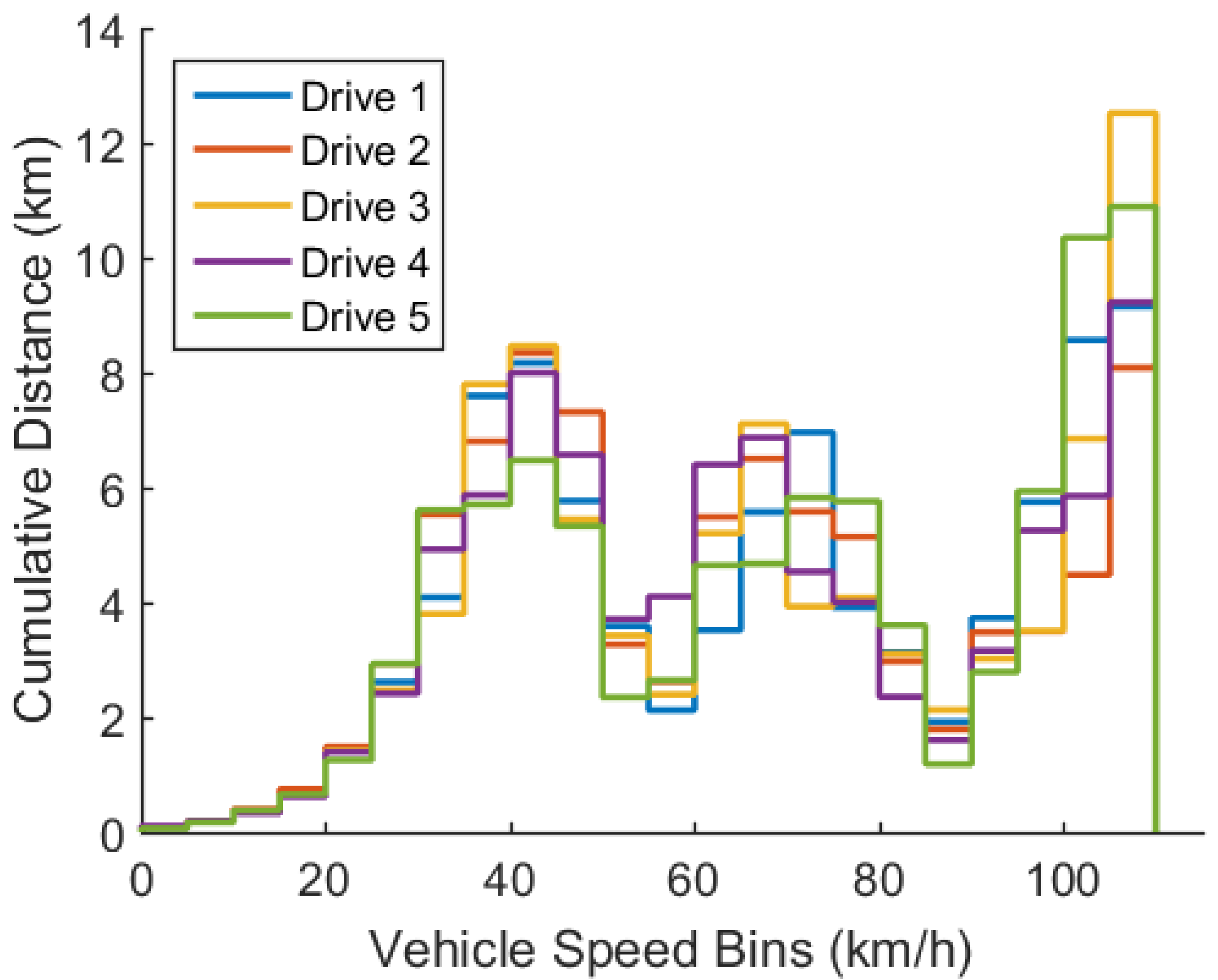
An interesting artefact of driving to meet the regulation requirements is the avoidance of the boundary vehicle speeds, 60 km/h and 90 km/h. During urban driving care is taken to not exceed 60 km/h and hence change the classification of the section to rural, and similarly during the rural portion of the drive care is taken to drive above 60 km/h to not build instantaneous urban driving and potentially produce a failed drive, such as Drive 2. Similarly, during the motorway section care is usually taken to keep the vehicle above 90 km/h and especially above 60 km/h. Figure 7 and Figure 8 show the vehicle speed residency for all 5 drives binned into vehicle speeds ranging from 0 to 115 km/h in 5 km/h increments for both the time residency and the distance traveled. Clearly seen is a dip in residency around 60 km/h and 90 km/h.
Drive 2, shows the highest residency in the 55–60 km/h bin of all the drives, and Drive 4, showed the second highest residency in that bin. Given the narrower driving range, effectively only speed limits of 100 and 110 km/h, the motorway bins have a greater residency with respect to distance than the others. Owing to the increased instantaneous urban driving on Drive 2, the motorway speed residencies are the lowest for this drive. A similar effect for the higher rural speeds is evident for Drive 4. Given that the distances covered in the 3 sections are roughly equal, with respect to time the motorway bins do not have as high a residency as the lower speed bins, particularly those of the urban section. Likewise, the high time residency in the 0–5 km/h bin, Figure 7, is not represented in the distance traveled plot, Figure 8.
Barlow et al. [37], show several metrics for the evaluation of drive cycles. Selected for evaluation of the data here are a subset of those: number of stops per km, average stop duration, average distance between stops, proportions of time accelerating, cruising, decelerating, and idling, relative positive acceleration (RPA) and relative cubic speed (RCS). In the calculations, the vehicle will be considered idle when the vehicle speed is less than 1 km/h and acceleration will be calculated as follows:
where i is the ith time step and is contained between 2 and , where N represents the total number of samples, noting that the sample rate is 1 Hz and . The RPA is calculated as [37,38]:
where is the total distance traveled in meters, and the RCS is calculated as [37]:
Figure 9 shows the average number of stops per kilometer during the urban, rural, and motorway phases of the drive, by topographical map, and the total average number of stops per kilometer across the whole drive. The number of stops is fairly consistent across the drive attempts and shows that it is likely that on a given route the number of stops is somewhat predictable. What is interesting, however, is the huge difference between the drive attempts and the repeat of the urban section when driven normally. The urban portion of the route only has traffic lights during the first kilometer, thereafter all the stops are a consequence of traffic. A similar story is evident in Figure 10. Figure 10 is showing the average distance between stops, here there is also evidence of less traffic in Drive 3.
Figure 11 shows the average stop time (average idle time, where the vehicle speed is less than 1 km/h). The average stop period in the rural section was influenced by traffic lights, aside from Drive 1 the average stop period was fairly consistent in the rural section. The average stop period for the motorway section is a function of both traffic lights and traffic–the traffic lights in the motorway section were on the roads used to change from traveling north to south on the Pacific Motorway, rather than on the motorway itself. Drive 2 had significant average stop time because of traffic.
The proportion of time spent accelerating, decelerating, cruising, and idling are calculated using an acceleration threshold of 0.1 m/s.
The proportion of time cruising in the urban period ranged from 21.0% to 25.5%. Time spent accelerating during a road cycle has been shown to be positively correlated with increased emissions [39]. Across the tests there were 31–40 idle events. Each idle event, must be followed by a low-speed acceleration event. Therefore, it can be inferred that the number of idle events will likely have an impact on overall emissions. Moreover, drives with less idle events have less opportunity for the exhaust to cool down and therefore challenge the after-treatment systems less. After-treatment systems operate optimally within a specific temperature range [40]. Therefore, it could be concluded that there is significant advantage in ensuring a route has the least opportunity for idle events as the regulation allows. Figure 12 show the proportion of time accelerating, decelerating, cruising, and idling during the urban section of the route.
The RPA has been shown to be an effective means of cycle comparison as it can be interpreted as the specific acceleration work of the trip [39,41]. Over the urban section of this route, the RPA ranged between 0.1627 and 0.1896 m/s. The narrow range is suggestive that the driving style across this section of the route did not differ significantly from drive-to-drive.
Related to the power demand, the RCS is a potentially interesting parameter to investigate when assessing the dynamics of a drive. As the resistive force on a vehicle from the aerodynamic drag is velocity dependent, the RCS has the potential as a parameter to allow a comparison between drive cycles based on aerodynamic force. Across the urban portion, the RCS ranged from 116.36 to 124.63 m/s. To evaluate the dynamics of the drive, it is also interesting to restrict the calculation to positive acceleration, relative positive cubic speed (RPCS).
The RPCS across the urban section ranged from 59.09 to 67.44 m/s, also indicative that the driving style did not vary substantially.
6. Conclusions
This paper has discussed the route design requirements of Commission Regulation (EU) 2018/1832 of 5 November 2018 [36] including the difficulties and limitations associated with designing a route to the meet the outlined boundary conditions. It has been shown that the 2 most difficult portions of the route to meet, in the design phase, are the requirement to show driving above 100 km/h for at least 5 min (requiring a motorway section speed limited at 110 km/h or greater) and locating a sufficiently long enough rural section. A methodology to design a compliant route was introduced and detailed in this paper using the development of a route on the Gold Coast in Queensland, Australia as a case study.
The designed route was driven 5 times to allow comparison between drives. The following was observed:
- It is possible to design a route that meets both instantaneous and topographical map section shares
- Shown was that traffic during the rural or motorway sections can significantly increase the instantaneous share of urban driving
- Over the urban section, a significant difference in average urban driving speed, idle share, average distance between stops, number of stops and average stopping time between the 5 drives was observed
- The use of established driving dynamic metrics, RPA and RPCS, showed that the style in which the vehicle was operated did not change significantly between drives, including the more naturally driven urban only drive.
Author Contributions
The experiment design and data collection performed by T.B.; analysis and manuscript preparation by T.B. and A.Z.
Funding
This research received no external funding.
Acknowledgments
Great thanks are extended to Stephen Maurer for his invaluable assistance in setting up the GPS device and the Raspberry Pi unit. Additionally, thanks are extended to Christine Ough and Brian and Lavinia Dack for their generous hospitality during the trip to Queensland to collect the data for this work.
Conflicts of Interest
The authors declare no conflict of interest.
References
- European Environmental Agency. EEA Report No 12/2018 Air Quality in Europe. Available online: https://www.eea.europa.eu/publications/air-quality-in-europe-2018 (accessed on 22 May 2019).
- Hooftman, N.; Messagie, M.; Mierlo, J.V.; Coosemans, T. A review of the European passenger car regulations—Real driving emissions vs local air quality. Renew. Sustain. Energy Rev. 2018, 86, 1–21. [Google Scholar] [CrossRef]
- Yue, X.; Wu, Y.; Hao, J.; Pang, Y.; Ma, Y.; Li, Y.; Li, B.; Bao, X. Fuel quality management versus vehicle emission control in China, status quo and future perspectives. Energy Policy 2015, 79, 87–98. [Google Scholar] [CrossRef]
- Yang, L.; Franco, V.; Mock, P.; Kolke, R.; Zhang, S.; Wu, Y.; German, J. Experimental assessment of NOx emissions from 73 Euro 6 diesel passenger cars. Environ. Sci. Technol. 2015, 49, 14409–14415. [Google Scholar] [CrossRef] [PubMed]
- Cha, J.; Lee, J.; Chon, M. Evaluation of real driving emissions for Euro 6 light-duty diesel vehicles equipped with LNT and SCR on domestic sales in Korea. Atmos. Environ. 2019, 196, 133–142. [Google Scholar] [CrossRef]
- Prati, M.; Costagliola, M.; Zuccheroso, A.; Napolitano, P. Assessment of Euro 5 diesel vehicle NOx emissions by laboratory and track testing. Environ. Sci. Pollut. Res. 2019, 26, 10576–10586. [Google Scholar] [CrossRef] [PubMed]
- Ramos, A.; Muñoz, J.; Andrés, F.; Armas, O. NOx emissions from diesel light duty vehicle tested under NEDC and real-word driving conditions. Transp. Res. Part Transp. Environ. 2018, 63, 37–48. [Google Scholar] [CrossRef]
- Luján, J.; Bermúdez, V.; Dolz, V.; Monsalve-Serrano, J. An assessment of the real-world driving gaseous emissions from a Euro 6 light-duty diesel vehicle using a portable emissions measurement system (PEMS). Atmos. Environ. 2018, 174, 112–121. [Google Scholar] [CrossRef]
- Degraeuwe, B.; Weiss, M. Does the New European Driving Cycle (NEDC) really fail to capture the NOX emissions of diesel cars in Europe? Environ. Pollut. 2017, 222, 234–241. [Google Scholar] [CrossRef]
- RDW. RDW Emission Test Programme. Available online: https://www.rdw.nl/-/media/rdw/rdw/pdf/sitecollectiondocuments/over-rdw/rapporten/rdw-emission-test-programme-english.pdf (accessed on 22 May 2019).
- GOV.UK 2016. Vehicle Emissions Testing Programme. Available online: https://assets.publishing.service.gov.uk/government/uploads/system/uploads/attachment_data/file/548148/vehicle-emissions-testing-programme-web.pdf (accessed on 22 May 2019).
- Marotta, A.; Pavlovic, J.; Ciuffo, B.; Serra, S.; Fontaras, G. Gaseous Emissions from Light-Duty Vehicles: Moving from NEDC to the New WLTP Test Procedure. Environ. Sci. Technol. 2015, 49, 8315–8322. [Google Scholar] [CrossRef]
- O’Driscoll, R.; ApSimon, H.; Oxley, T.; Molden, N.; Stettler, M.; Thiyagarajah, A. A Portable Emissions Measurement System (PEMS) study of NOX and primary NO2 emissions from Euro 6 diesel passenger cars and comparison with COPERT emission factors. Atmos. Environ. 2016, 145, 81–91. [Google Scholar] [CrossRef]
- European Commission. Commission Regulation (EU) 2016/427 of 10 March 2016 Amending Regulation (EC) No 692/2008 as Regards Emissions From Light Passenger and Commercial Vehicles (Euro 6). Available online: https://eur-lex.europa.eu/legal-content/EN/TXT/?uri=OJ:L:2016:082:TOC (accessed on 22 May 2019).
- Pelkmans, L.; Debal, P. Comparison of on-road emissions with emissions measured on chassis dynamometer test cycles. Transp. Res. Part Transp. Environ. 2006, 11, 233–241. [Google Scholar] [CrossRef]
- Kadijk, G.; Ligterink, N. TNO 2012 R10237 Road Load Determination of Passenger Cars. Available online: https://ermes-group.eu/web/system/files/filedepot/9/2012-TNO-road-load-060-DTM-02014.pdf (accessed on 22 May 2019).
- van Mensch, P.; Ligterink, N.; Cuelenaere, R. The effect on road load due to variations in valid coast down tests for passenger cars. In Proceedings of the 20th International Transport and Air Pollution Conference, Graz, Austria, 18–19 September 2014. [Google Scholar]
- Martin, N.; Bishop, J.; Choudhary, R.; Boies, A. Can UK passenger vehicles be designed to meet 2020 emissions targets? A novel methodology to forecast fuel consumption with uncertainty analysis. Appl. Energy 2015, 157, 929–939. [Google Scholar] [CrossRef] [Green Version]
- Mellios, G.; Hausberger, S.; Keller, M.; Samaras, Z.; Ntziachristos, L. Parameterisation of Fuel Consumption and CO2 Emissions of Passenger Cars and Light Commercial Vehicles for Modelling Purposes. European Commission Joint Research Centre Technical Report EUR 24927 EN. Publ. Off. Eur. Union 2011, 24927, 1–116. [Google Scholar]
- Franco, V.; Kousoulidou, M.; Muntean, M.; Ntziachristos, L.; Hausberger, S.; Dilara, P. Road vehicle emission factors development: A review. Atmos. Environ. 2013, 70, 84–97. [Google Scholar] [CrossRef]
- Weiss, M.; Bonnel, P.; Hummel, R.; Provenza, A.; Manfredi, U. On-Road Emissions of Light-Duty Vehicles in Europe. Environ. Sci. Technol. 2011, 45, 8575–8581. [Google Scholar] [CrossRef] [PubMed]
- Kousoulidou, M.; Fontaras, G.; Ntziachristos, L.; Bonnel, P.; Samaras, Z.; Dilara, P. Use of portable emissions measurement system (PEMS) for the development and validation of passenger car emission factors. Atmos. Environ. 2013, 64, 329–338. [Google Scholar] [CrossRef]
- Duarte, G.; Goncalves, G.; Farias, T. Analysis of fuel consumption and pollutant emissions of regulated and alternative driving cycles based on real-world measurements. Transp. Res. Part Transp. Environ. 2016, 44, 43–54. [Google Scholar] [CrossRef]
- Samuel, S.; Austin, L.; Morrey, D. Automotive test drive cycles for emission measurement and real-world emission levels—A review. Proc. Inst. Mech. Eng. Part J. Automob. Eng. 2002, 216, 555–564. [Google Scholar] [CrossRef]
- Tutuianu, M.; Bonnel, P.; Ciuffo, B.; Haniu, T.; Ichikawa, N.; Marotta, A.; Pavlovic, J.; Steven, H. Development of the World-wide harmonized Light duty Test Cycle (WLTC) and a possible pathway for its introduction in the European legislation. Transp. Res. Part Transp. Environ. 2015, 40, 61–75. [Google Scholar] [CrossRef]
- Pavlovic, J.; Marotta, A.; Ciuffo, B. CO2 emissions and energy demands of vehicles tested under the NEDC and the new WLTP type approval test procedures. Appl. Energy 2016, 177, 661–670. [Google Scholar] [CrossRef]
- Pavlovic, J.; Ciuffo, B.; Fontaras, G.; Valverde, V.; Marotta, A. How much difference in type-approval CO2 emissions from passenger cars in Europe can be expected from changing to the new test procedure (NEDC vs. WLTP)? Transp. Res. Part Policy Pract. 2018, 111, 136–147. [Google Scholar] [CrossRef]
- Tsiakmakis, S.; Fontaras, G.; Cubito, C.; Pavlovic, J.; Anagnostopoulos, K.; Ciuffo, B. From NEDC to WLTP: Effect on the Type-Approval CO2 Emissions Of Light-Duty Vehicles. Available online: https://core.ac.uk/download/pdf/132627125.pdf (accessed on 22 May 2019).
- Pavlovic, J.; Marotta, A.; Ciuffo, B.; Serra, S.; Fontaras, G.; Anagnostopoulos, K.; Tsiakmakis, S.; Arcidiacono, V.; Hausberger, S.; Silberholz, G. Correction of test cycle tolerances: evaluating the impact on CO2 results. Transp. Res. Proc. 2016, 14, 3099–3108. [Google Scholar] [CrossRef]
- Andersson, J.; May, J.; Favre, C.; Bosteels, D.; de Vries, S.; Heaney, M.; Keenan, M.; Mansell, J. On-Road and Chassis Dynamometer Evaluations of Emissions from Two Euro 6 Diesel Vehicles. SAE Int. J. Fuels Lubr. 2014, 7, 919–934. [Google Scholar] [CrossRef]
- Rubino, L.; Bonnel, P.; Hummel, R.; Krasenbrink, A.; Manfredi, U.; De Santi, G.; Perotti, M.; Bomba, G. PEMS Light-Duty Vehicles Application: Experiences in Downtown Milan. Available online: https://www.sae.org/publications/technical-papers/content/2007-24-0113/ (accessed on 22 May 2019).
- European Commission. Commission Regulation (EU) 692/2008 of 18 July 2008 amending Regulation (EC) No 715/2007 of the European Parliament and of the Council on type-approval of motor vehicles with respect to emissions from light passenger and commercial vehicles (Euro 5 and Euro 6) and on access to vehicle repair and maintenance information. Off. J. Eur. Union 2008, 51, 1–136. [Google Scholar]
- Weiss, M.; Bonnel, P.; Kuhlwein, J.; Provenza, A.; Lambrecht, U.; Alessandrini, S.; Carriero, M.; Colombo, R.; Forni, F.; Lanappe, G.; et al. Will Euro 6 reduce the NOX emissions of new diesel cars?—Insights from on-road tests with Portable Emissions Measurement Systems (PEMS). Atmos. Environ. 2012, 62, 657–665. [Google Scholar] [CrossRef]
- Klier, T.; Linn, J. The VW Scandal and Evolving Emissions Regulations. Chic. Fed Lett. 2016, 357, 1. [Google Scholar]
- European Commission. Commission Regulation (EU) 2017/1154 of 7 June 2017 Amending Regulation (EU) 2017/1151 Supplementing Regulation (EC) No 715/2007 of the European Parliament and of the Council on Type-Approval of Motor Vehicles With Respect to Emissions from Light Passenger and Commercial Vehicles (Euro 5 and Euro 6) and on Access to Vehicle Repair and Maintenance Information, Amending Directive 2007/46/EC of the European Parliament and of the Council, Commission Regulation (EC) No 692/2008 and Commission Regulation (EU) No 1230/2012 and Repealing Regulation (EC) No 692/2008 and Directive 2007/46/EC of the European Parliament and of the Council as Regards Real-Driving Emissions from Light Passenger and Commercial Vehicles (Euro 6). Available online: https://publications.europa.eu/en/publication-detail/-/publication/a6a9f402-a8cc-11e7-837e-01aa75ed71a1 (accessed on 22 May 2019).
- European Commission. Commission Regulation (EU) 2018/1832 of 5 November 2018 amending Directive 2007/46/EC of the European Parliament and of the Council, Commission Regulation (EC) No 692/2008 and Commission Regulation (EU) 2017/1151 for the purpose of improving the emission type approval tests and procedures for light passenger and commercial vehicles, including those for in-service conformity and real-driving emissions and introducing devices for monitoring the consumption of fuel and electric energy. Off. J. Eur. Union 2018, 59. Available online: https://eur-lex.europa.eu/eli/reg/2018/1832/oj (accessed on 22 May 2019).
- Barlow, T.; Latham, S.; McCrae, I.; Boulter, P. A Reference Book of Driving Cycles for Use in the Measurement of Road Vehicle Emissions. Available online: http://worldcat.org/isbn/9781846088162 (accessed on 22 May 2019).
- De Haan, P. Modelling fuel consumption and pollutant emissions based on real-world driving patterns: The HBEFA apprach. Int. J. Environ. Pollut. 2004, 22, 240–258. [Google Scholar] [CrossRef]
- Pathak, S.; Sood, V.; Singh, Y.; Channiwala, S. Real world vehicle emissions: Their correlation with driving parameters. Transp. Res. Part Transp. Environ. 2016, 44, 157–176. [Google Scholar] [CrossRef]
- Franco, V.; Zacharopoulou, T.; Hammer, J.; Schmidt, H.; Mock, P.; Weiss, M.; Samaras, Z. Evaluation of Exhaust Emissions from Three Diesel-Hybrid Cars and Simulation of After-Treatment Systems for Ultralow Real-World NOx Emissions. Environ. Sci. Technol. 2016, 50, 13151–13159. [Google Scholar] [CrossRef]
- Sileghem, L.; Bosteels, D.; May, J.; Favre, C.; Verhelst, S. Analysis of vehicle emission measurements on the new WLTC, the NEDC and the CADC. Transp. Res. Part Transp. Environ. 2014, 32, 70–85. [Google Scholar] [CrossRef] [Green Version]
Figure 1.
New European Driving Cycle (NEDC).

Figure 2.
World-wide harmonized light duty cycle (WLTC) Class 3 Version 5.

Figure 3.
Actual vehicle speed, as measured by a GPS device, against the displayed nominal vehicle speed of a 2016 2.5 ℓ Toyota Camry.
Figure 3.
Actual vehicle speed, as measured by a GPS device, against the displayed nominal vehicle speed of a 2016 2.5 ℓ Toyota Camry.

Figure 4.
Rural section of the driving route.

Figure 5.
Motorway section of the driving route.

Figure 6.
Urban section of the driving route.

Figure 7.
Vehicle speed residency across each drive with respect to time.

Figure 8.
Vehicle speed residency across each drive with respect to distance traveled.

Figure 9.
Average number of stops per kilometer for each section of the drive, by topographical map.
Figure 9.
Average number of stops per kilometer for each section of the drive, by topographical map.

Figure 10.
Average distance between stops for each section of the drive, by topographical map.

Figure 11.
Average stop time for each section of the drive, by topographical map.

Figure 12.
Proportion of time accelerating, cruising, decelerating, and idling during the urban section of the route for each drive.
Figure 12.
Proportion of time accelerating, cruising, decelerating, and idling during the urban section of the route for each drive.


Table 1.
Trip requirements for a valid RDE test.
| Total Trip Duration | 90–120 min | ||
|---|---|---|---|
| Cumulative Positive Elevation Gain (Urban and Total Trip | <1200 m/100 km | ||
| Start/End Test Elevation Difference | ≤100 m | ||
| Driving portion | Urban | Rural | Motorway |
| speed ≤ 60 km/h | 60 < speed ≥ 90 km/h | speed > 90 km/h | |
| Average speed | 15 < speed < 40 km/h | - | - |
| Distance share | 29–44% | 23–43% | 23–43% |
| Minimum distance | 16 km | 16 km | 16 km |
| Individual stop | ≤300 s | - | - |
| Total stop time | 6–30% of urban time | - | - |
| Speed > 100 km/h | - | - | ≥5 min |
| Speed > 145 km/h | - | - | <3% of motorway time |
© 2019 by the authors. Licensee MDPI, Basel, Switzerland. This article is an open access article distributed under the terms and conditions of the Creative Commons Attribution (CC BY) license (http://creativecommons.org/licenses/by/4.0/).
Share and Cite
MDPI and ACS Style
Bodisco, T.; Zare, A. Practicalities and Driving Dynamics of a Real Driving Emissions (RDE) Euro 6 Regulation Homologation Test. Energies 2019, 12, 2306. https://doi.org/10.3390/en12122306
AMA Style
Bodisco T, Zare A. Practicalities and Driving Dynamics of a Real Driving Emissions (RDE) Euro 6 Regulation Homologation Test. Energies. 2019; 12(12):2306. https://doi.org/10.3390/en12122306
Chicago/Turabian StyleBodisco, Timothy, and Ali Zare. 2019. "Practicalities and Driving Dynamics of a Real Driving Emissions (RDE) Euro 6 Regulation Homologation Test" Energies 12, no. 12: 2306. https://doi.org/10.3390/en12122306
Note that from the first issue of 2016, this journal uses article numbers instead of page numbers. See further details here.