Characterization of In-Cylinder Combustion Temperature Based on a Flame-Image Processing Technique

Abstract

The analysis of in-cylinder combustion temperatures using flame image processing technology is reliable. This method can accurately, intuitively, and in real time obtain the temperature field distribution law of the combustion flame in the cylinder, so we can more deeply understand the characteristics of the combustion process of internal combustion engines. In this paper, a high-speed charge-coupled device (CCD) camera is used to record an in-cylinder combustion image, which is calculated and corrected according to the principle of three primary color temperature measurement, and the temperature field distribution of the combustion flame in the diesel engine cylinder is analyzed in detail. In addition, the temperature of the typical combustion flame images under the open-cycle and closed cycle conditions is compared by the CMS2002 measurement and MATLAB program, respectively. The results show that the accuracy of the MATLAB program is acceptable in general but not entirely acceptable in a few ways.

1. Introduction

Combustion is a very complex chemical reaction, and the flame’s combustion temperature is an important state parameter that reflects the combustion process. It is crucial to study the heat generated by combustion and the heat transfer in space, which affects the dynamics, economy, and emissions of internal combustion engines. Therefore, stable combustion is of great significance to the current topic of energy conservation and emission reduction.

Common methods for measuring the temperature in the cylinder are the contact and non-contact types. When measuring the temperature distribution in the cylinder, the contact temperature measurement method has a large difference from the actual temperature due to the disturbance of the temperature sensing element to the temperature field, the thermal inertia of the sensor and the limitation of the temperature measurement area. Non-contact methods, such as the optical temperature measurement, have the advantage of a wide measuring range, transient response, and high precision, which have made them widely used in temperature measurement in internal combustion engines.

The charge-coupled device (CCD)-based optical temperature measurement technology combines the traditional radiation principle, modern photoelectric conversion principle, and digital image processing technology, and has the advantage of a non-contact, fast response, small error, and real-time dynamic measurement. The working principle of the CCD image sensor is [1,2,3,4,5]: When external light illuminates the pixel array of the sensor, and the optical signal is converted into an electrical signal, which is a photoelectric effect. At this time, a moving charge is generated on the internal silicon of the CCD, and a current is formed. The corresponding pixel unit is selected by the logic controller according to the nature of the obtained current, and the overall image is represented by an electrical form signal. The electrical signal is passed to the A/D converter, which, in turn, is converted to a digital signal, a discrete value image signal (color image).

CCD as an important sensor that is easy to connect with a computer and has a wide range of applications in temperature field simulation, velocity measurement, and spectral analysis. In 1932, Hottel and Broughton [6] used the two-color method to measure flame temperature for the first time. This study pioneered two-color temperature measurement. In this experiment, they tried to get the temperature and total emissivity of the luminous flame. Because of the limitations of the conditions at that time, this method has many shortcomings, such as the inability to realize real-time measurements. In 1979, Cashdollar [7] used a pyrometer to measure the continuum radiation from particles in a flame at three wavelengths (0.8 μm, 0.9 μm, and 1.0 μm) and calculated the particle temperature from the radiation data using the Planck equation. The HAICS-3000 system was developed by Hitachi in 1985. Flame image recognition technology was used to obtain the distribution of the whole flame temperature field [8]. Abe et al. [9] proposed an indirect method to estimate light source color or the correlated color temperature of illuminants. The correlated color temperature of the light source illuminating the color chips is estimated. Ito et al. [10] presented a quantitative characterization of propane premixed flame color and its applications in their work. Detailed relations between flame colors and flame spectra are investigated in the specific range of the air/fuel ratio. In 1993, BHP Billiton researcher Chen et al. [11] showed how nearly infrared CCD temperature measurement technology was applied to the steel industry. In 1995, Hsu et al. [12] used the enhanced CCD to measure the flame temperature of liquid metal and got some results, but the error was large. In 1996, Skarman et al. [13] used CCD to take a hologram of fluid and reconstruct the three-dimensional temperature field of the fluid by image processing technology. Because of the performance of CCD, the experimental results were not satisfactory. Panagiotou et al. [14] used a three-color near-infrared optical pyrometer, with wavelengths centered at 998, 810, and 640 nm, to monitor the combustion of polymer particles. Zhao et al. [15] used laser induced incandescence (LII) to image the two-dimensional soot distribution. Lu et al. [16] of Greenwich University developed a device to measure the temperature distribution of pulverized coal flame and the concentration of soot in 2001. The experimental results in a furnace show that the device can effectively measure the instantaneous flame temperature and soot concentration. In 2003, Sutter et al. [17] used CCD to measure the temperature of the radiator by measuring the monochromatic light emitted from the surface of the object. This method was used to measure the temperature of high-speed cutting tools, and the results were satisfactory. Brisley et al. [18] combined the image-processing techniques and two-color radiation thermometry for temperature measurement of combustion flame in 2005. Lu et al. [19] presented an imaging-based multicolor pyrometric system for the monitoring of temperature and its distribution in a coal-fired flame. Panditrao and Rege [20] proposed a novel noncontact temperature measurement technique using a consumer-grade digital still camera. Wu et al. [21] employed an intensified CCD camera coupled with bandpass filters to capture the quasi-steady state flame emissions of diesel (No. 2) and a diesel-gasoline blend (dieseline: 80% diesel and 20% gasoline by volume) at 430 nm and 470 nm bands in 2016. Liu and Liu [22] presented an inverse analysis based on the flame emission spectrum technique for the simultaneous reconstruction of two-dimensional (2D) temperature and the concentration fields of soot and metal-oxide nanoparticles in the asymmetric nanofluid fuel flames by means of CCD cameras in 2018. The technique was successfully used for measuring the temperature distribution of different industrial applications, like in a muffle furnace, salt bath furnace, or induction furnace.

However, the above studies used zero-dimensional calibration, in other words, a homogeneous temperature object, to examine the accuracy. There is a difference between the radiation characteristics of the hot metal and the diesel flame. Further, there may be some impacts while processing a two-dimensional image as the program was calibrated zero-dimensionally. The CMOS or CCD sensors with custom filters (often narrow bandwidth filters) are needed for traditional monochrome or bichrome temperature measurement, which would increase the cost of equipment and reduce the generality of data processing. This paper verifies the feasibility of temperature measurement with ordinary cameras, which reduce the cost of measurement and benefit from the two-color method. The calculation program can be used to process diesel flame photographs taken by the same type of cameras in order to obtain more basic data. In addition, the flame temperature characterization of the diesel engine under open-cycle and closed cycle conditions, which represents the working conditions of a submarine, was needed to be further studied and discussed [23]. In this study, some typical flame images of in-cylinder combustion were recorded using a high-speed CCD camera, and the combustion temperature was calculated and corrected by a three-primary color temperature method. Finally, the temperature of the typical combustion flame images under the open-cycle and closed cycle conditions was compared by the CMS2002 (University of Science and Technology of China, Hefei, China) measurement and the MATLAB (MathWorks, Natick, USA) program, respectively.

2. Temperature Measurement Principle and Test Device

When measuring temperature using a conventional method, such as the thermocoupling, only the temperature value at a certain point in the flame region can be measured. It is more desirable for researchers to obtain the distribution of the overall temperature field, which is difficult to achieve via traditional temperature measurement methods. The flame field consists of countless pixels, which modern digital technology has studied and developed. Each pixel on the image captured by the digital camera is stored with a specific primary color value. Each pixel has a unique primary color value, which corresponds to a specific temperature value. In this way, the development of high-speed cameras has laid a solid foundation for the formation of the trichromatic temperature measurement theory.

2.1. Optical Principle

Light waves have energy. The wavelength of light that can be seen by the human eye is between 380 nm and 780 nm. The visible light is divided into six colors, which are red, orange, yellow, green, blue, and purple according to the wavelength. According to the research, the energy of light waves increases with the decrease of wavelength, and different wavelengths represent different energies. Thus, the color seen by the human eye is recognized. The characteristics of light can be described by the temperature [6]. Then, one can react to different energies, judge the temperature, and finally realize the actual temperature of the object.

2.2. Radiation Principle

Any object, as long as the temperature is above absolute zero, transmits energy outward in the form of electromagnetic waves. This way of transmitting energy is called radiation. The flame is accompanied by a strong radiant energy transfer process during the combustion process. A blackbody is an idealized object that absorbs all incident radiation. The spectral distribution of the radiation intensity of blackbody emission is determined by Planck:

$$E_b\left(\lambda , T\right)=\frac{2h{C}_0^2}{{\lambda }^5\left[\exp \left(\frac{h{C}_0}{\lambda pT}\right)-1^{}\right]}$$

(1)

where h = 6.6256 × 10⁻³⁴ J·s and p = 1.3805 × 10⁻²³ J/K are the common constants of Planck and Boltzmann, respectively. C₀ = 2.998 × 10⁸ m/s is the speed of light in vacuum. T is the absolute temperature in K.

Since the black body is a diffuse reflector, the spectral emission power can be expressed as

$$E_b\left(\lambda , T\right)=\frac{C_1}{{\lambda }^5\left[\exp \left(\frac{C_2}{\lambda T}\right)-1^{}\right]}$$

(2)

where C₁ = 3.7418 × 10⁻¹⁶ W·m² is called Planck’s first radiation constant and C₂ = 1.4388 × 10⁻² m·K is called Planck’s second radiation constant. E_b(λ, T) represents the blackbody radiation intensity at a wavelength of λ and a temperature of T.

The black body is just an ideal surface. For a general object, its radiation can be expressed as

$$E\left(\lambda , T\right)={\epsilon }_{\lambda }\frac{C_1}{{\lambda }^5\left[exp\left(\frac{C_2}{\lambda T}\right)-1\right]}$$

(3)

where C₁ and C₂ are Planck’s first constant and second constant, respectively. E(λ, T) is the monochromatic radiation power. ε_λ is the monochromatic emissivity and λ is the wavelength. The monochromatic emissivity of an object is a function of temperature and wavelength:

$${\epsilon }_{\lambda }=f\left(\lambda , T\right)$$

(4)

It can be seen from Equations (3) and (4) that the radiated power of an object is related to its temperature and radiance. Therefore, in simple terms, the visible light color radiated by an object can be determined by the temperature and emissivity of the object.

The flame’s monochromatic radiance is obtained from the theory of small particle scattering, which can be expressed as:

$${\epsilon }_{\lambda , r}=1-\exp \left(-\frac{kl}{{\lambda }^{\alpha }}\right)$$

(5)

The constant α in the equation is determined by the wavelength range and α = 1.39 in the wavelength range of the visible light. k is the absorption coefficient and l is the geometric thickness of the flame in the direction of the optical axis of the sensor.

According to the Planck Equation (3), for any color image, the following equation can be determined:

$$\{\begin{array}{c}E\left({\lambda }_1, T\right)={\epsilon }_{{\lambda }_1}\frac{C_1}{{\lambda }_1^5\left[\exp \left(\frac{C_1}{{\lambda }_{1}T}\right)-1^{}\right]}\\ E\left({\lambda }_2, T\right)={\epsilon }_{{\lambda }_2}\frac{C_1}{{\lambda }_2^5\left[\exp \left(\frac{C_1}{{\lambda }_{2}T}\right)-1^{}\right]}\\ ·\\ ·\\ ·\\ E\left({\lambda }_n, T\right)={\epsilon }_{{\lambda }_n}\frac{C_1}{{\lambda }_n^5\left[\exp \left(\frac{C_1}{{\lambda }_{n}T}\right)-1^{}\right]}\end{array}$$

(6)

The radiation intensity of the object can be obtained by solving the above-mentioned overdetermined equations. Thus, its color is expressed, and finally the temperature distribution of the object is determined.

2.3. Principle of Trichromatic Temperature Measurement

Through the color matching experiment [15], it can be obtained that red, green, and blue are the most ideal three primary colors, which are represented by R, G, and B, respectively. Whether it is black, white, or various colors, unsaturated colors can be formulated through these three primary colors. In the process of preparing the color, it is not required that the prepared light be exactly the same as the original monochromatic light, as only the chromaticity and the brightness are required to be consistent.

The transmittances of the three color filters in the Bayer array for light of wavelength λ are represented by r(λ), g(λ), and b(λ), respectively. P(λ) represents the luminous flux of wavelength λ in the incident light, and the distribution color coefficient equation can be used to calculate:

$$\{\begin{array}{c}\mathrm{R}={{\displaystyle \int }}_{380}^{780}\overline{r}\left(\lambda \right)P\left(\lambda \right)d\lambda \\ \mathrm{G}={{\displaystyle \int }}_{380}^{780}\overline{g}\left(\lambda \right)P\left(\lambda \right)d\lambda \\ \mathrm{B}={{\displaystyle \int }}_{380}^{780}\overline{b}\left(\lambda \right)P\left(\lambda \right)d\lambda \end{array}$$

(7)

In general, objects can be considered to obey Planck’s law. If (3) is substituted into (7), then the color light coefficient of objects can be written as:

$$\{\begin{array}{c}\mathrm{R}={{\displaystyle \int }}_{380}^{780}\overline{r}\left(\lambda \right){\epsilon }_{\lambda }\frac{C_1}{{\lambda }^5\left[\exp \left(\frac{C_1}{\lambda T}\right)-1^{}\right]}d\lambda \\ \mathrm{G}={{\displaystyle \int }}_{380}^{780}\overline{g}\left(\lambda \right){\epsilon }_{\lambda }\frac{C_1}{{\lambda }^5\left[\exp \left(\frac{C_1}{\lambda T}\right)-1^{}\right]}d\lambda \\ \mathrm{B}={{\displaystyle \int }}_{380}^{780}\overline{b}\left(\lambda \right){\epsilon }_{\lambda }\frac{C_1}{{\lambda }^5\left[\exp \left(\frac{C_1}{\lambda T}\right)-1^{}\right]}d\lambda \end{array}$$

(8)

According to the above formula, the color of all objects due to their own radiation depends on the radiation spectrum of the object. By selecting the emissivity model, the color light coefficient of the object is calculated, and the temperature of the object is finally obtained. This is the temperature measurement principle of the three primary colors.

It should be pointed out that due to the existence of optical elements and photoelectric conversion system in the measurement system, there will be errors between the measured temperature and the actual temperature. In order to ensure the accuracy of the temperature measurement, the color flame image must be calibrated [16]. The calibration is mainly used to correct the RGB tricolor values so that it can correctly reflect the spectral intensity of the radiated object under the RGB representative wavelength.

2.4. Test Bench

The test bench is shown in Figure 1, where 1 is a CY-YD 205 quartz piezoelectric pressure sensor for cylinder pressure sensor and 3 is a Kistler 5011 (Kistler Instrument China Ltd., Shanghai, China) charge amplifier matched with it; 2 is the injector; 4 is FASTCAM-ultima512 high-speed camera produced by PHOTRON Company; 5 is the data acquisition computer, which includes a frame grabber. The optical engine was redesigned based on a ZS195 (Changchai Co., Ltd., Changzhou, China) direct injection diesel engine, which is a horizontal single-cylinder water-cooled direct injection diesel engine with a diameter of 95 mm, as well as a stroke of 115 mm and a compression ratio of 17. The engine has a calibrated power of 8.8 kW at 2200 rpm, with maximum torque of 50 N m at 1600 rpm. The combustion chamber is ω-shaped. The cylinder head is modified to fit the pressure sensor (1) and drill a hole to install the quartz glass (6) to let the light pass through. Further, there is no way to preserve the cooling channels within the cylinder head, so the engine could not operate for too long or else the cylinder head would be overheated, or the quartz glass would be covered by soot. There is a frequency conversion motor (9) that is used to drive the engine to a designated speed before a fire and bear a load when the engine is operating. In order to ensure that the cooling water temperature is close to the actual working condition, an electrical heater is used to heat the cooling water before the test, and the water temperature is maintained at about 70 °C during the test. Number 7 is the flywheel, with teeth in the circle for the magnetoelectric speed sensor (8) to acquire the crankshaft angle. There were two sets of experiments: Series 1 means open cycle (normal air combustion condition) and series 2 means closed cycle (65% O₂ + 35% CO₂).

The high-speed CCD camera uses a FASTCAM-ultima512 high-speed camera produced by the PHOTRON Company of Japan. The lens is a NIKON SLR (Nikon Image Instrument Sales (China) Co., Ltd., Shanghai, China) camera lens. It communicates with the computer by using the IEEE 1394 interface. The sensor type is CCD, and the resolution can be adjusted to 512 × 512. The shooting speed is 2000 frames per second at full resolution and 3200 frames per second at a sub-frame state. In this experiment, the camera resolution was set to 128 × 128 and the shooting speed was 8000 frames per second. All components involved in radiation generation, propagation and reception were calibrated together, including the diesel flame, quartz glass, lens, camera, and, of course, air was not absent.

3. Results and Discussion

3.1. Analysis of Combustion Temperature Field

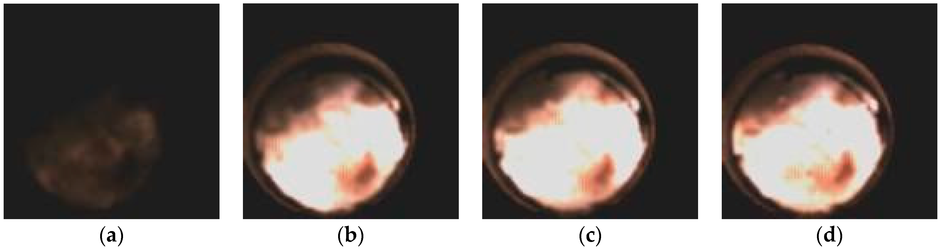
The flame image during the combustion process in the cylinder was obtained through experiments, and some images of special moments are extracted. The selected pictures, shown in Figure 2, were brought into the MATLAB program to obtain the results of the two-color method. Visual temperature field pictures and statistical maximum, minimum, and average values were recorded. In the figures, Figure 2 is the actual flame image, and Figure 3 is the temperature field image after calculation. In the open cycle, a complete cycle of optical engine visualization test result statistics is from 12,108 frames to 13,511 frames, the frame span is 1403 frames, and the corresponding time is 0.175375 seconds, from which instantaneous speed can be calculated as 684 rpm. The fuel ignites at the 3.43 crankshaft angle (°CA) after the top dead centre (TDC). The maximum heat release rate is 198.02 J/°CA at 10 °CA after TDC, the maximum pressure rise rate is 0.768 MPa/°CA at 11 °CA after TDC, and the maximum pressure is 6.12 MPa at 16 °CA after TDC.

It can be seen from

Table 1. Typical temperature of series 1 with MATLAB.

Temperature	Ignition (°C)	Maximum Pressure Rise Rate (°C)	Maximum Heat Release (°C)	Peak Pressure (°C)
Average	2200	1894	1894	1865
Maximum	2200	2734	2583	2475
Minimum	2200	1440	1439	1439
Quantity	124	9901	9864	9752

that the average temperature is about 1900 °C for all the times except the ignition moment. The area that is in fire keeps about 9800 pixels. Series 2 is for the typical crank angle moment of a closed cycle. In a closed cycle, the complete work cycle statistics of the optical engine visualization test ranged from 8852 frames to 10,069 frames, the frame span is 1217 frames, and the corresponding time is 0.152125 s, from which the instantaneous speed can be calculated as 789 rpm. The fuel ignites at 2.77 °CA after TDC, the pressure rise rate reaches the maximum value of 0.496 MPa/°CA at 5 °CA after TDC, and the heat release rate reaches the maximum value of 206.71 J/°CA at 6 °CA after TDC. The maximum pressure in the cylinder is 5.96 MPa at 15 °CA after TDC. From Table 1, we can see that the maximum and the minimum are both 2200 °C, which means that every pixel weighted has the same characteristic value. Then, it turns out that the r, g, and b values vary when the initial arrays are examined. Here are the two reasons that caused this error: one is that computational accuracy is not strong enough for this purpose. Another is that the program is based on the two-color method; the characteristic value is r/g, which means that the temperature will not change if the r/g is constant, while r, g and b vary.

From

Table 2. Typical temperature of series 2 with MATLAB.

Temperature	Ignition (°C)	Maximum Pressure Rise Rate (°C)	Maximum Heat Release (°C)	Peak Pressure (°C)
Average	1865	1902	1879	1893
Maximum	2475	2898	2393	2502
Minimum	1439	1439	1568	1439
Quantity	4976	9666	9679	9931

, it can be seen that the average temperature of the four processes calculated from Figure 4: the average temperature at all four moments is around 1900 °C, constantly. In addition, compared with Table 1, the mean value and maximum value of the two sets of temperatures measured at the same time of combustion in the two groups are close to each other, and the temperature obtained in each process is consistent with the fact. As can be seen from the temperature field in Figure 5, the yellow area represents a higher temperature and the blue area represents a lower temperature.

Figure 6 and Figure 7 processed with the CMS software as competition.

Table 3. Typical temperature of series 1 with CMS.

Temperature	Ignition (°C)	Maximum Pressure Rise Rate (°C)	Maximum Heat Release (°C)	Peak Pressure (°C)
Average	2051	1904	1897	1876
maximum	2076	2759	2973	2707
Minimum	2008	908	902	952
Quantity	124	9901	9864	9752

and

Table 4. Typical temperature of series 2 with CMS.

Temperature	Ignition (°C)	Maximum Pressure Rise Rate (°C)	Maximum Heat Release (°C)	Peak Pressure (°C)
Average	1846	1878	1875	1887
Maximum	2197	2956	2962	2435
Minimum	1502	940	897	899
Quantity	4976	9666	9679	9931

are the typical temperatures of the two series calculated by CMS2002.

3.2. Discussion

Figure 8 and

Table 5. Error of typical temperature based on CMS of series 1.

Temperature	Ignition (%)	Maximum Pressure Rise Rate (%)	Maximum Heat Release (%)	Peak Pressure (%)
Average	7.3	0.5	0.2	0.6
Maximum	6.0	9.1	13.1	8.6
Minimum	9.6	58.6	59.5	51.1

are the results of the air charge condition processed with the two software choices. It can be seen that the mean values of each picture in Figure 2, calculated with both programs, are equal, as the two mean value polylines coincide briefly. However, the differences are between the two maximums polylines, and also between the two minimum polylines. In the ignition moment, the differences is not as big as in the other three moments. Except for the maximum of the max pressure rise rate and peak pressure, the different valve of the typical temperature calculated with the two programs is about 400 °C. The maximum calculated with the CMS software is always bigger than that calculated with MATLAB software, and the minimum calculated with CMS is always smaller than that calculated with MATLAB software, while the difference is above 50 °C.

Figure 9 and

Table 6. Error of typical temperature based on CMS of series 2.

Temperature	Ignition (%)	Maximum Pressure Rise Rate (%)	Maximum Heat Release (%)	Peak Pressure (%)
Average	1.0	1.3	0.2	0.3
Maximum	12.7	1.9	19.2	2.8
Minimum	4.2	53.1	74.8	60

are the polylines of closed-cycle calculated with the two software. Similar to the condition of the air condition, the mean values are almost the same, and except for the maximums at the ignition moment, the maximum calculated with the CMS software is always bigger than that calculated with MATLAB software and the minimum calculated with CMS is always smaller than that calculated with MATLAB software, while the difference is above 50 °C.

Above all, the mean values are briefly the same. However, the maximums and the minimum tend to separate. Then, we can see from the temperature cloud pictures in Figure 3, Figure 5, Figure 6 and Figure 7 that the temperature represented by the majority of the area is relatively similar, which means that the different values above 200 °C only exist in a few pixels, so that the mean values coincide briefly.

Both methods take R > 34 as the identifying condition, so the pixel in a picture from Figure 2 or Figure 4 is taken into calculation or is not the same in the two methods, which can be seen from the amount of pixels taken into account; they are equal to the same pictures from Figure 2 and Figure 4. Thus, the difference between the two groups of outcomes of the two methods is because of the calculating formula. Ignoring the differences in maximums and minimums, the two groups fit quite well.

4. Conclusions

A calculating formula based on a two-color method for the camera is given, and pictures were taken while the optic engine operated. The program can analyse the temperature distribution with the image taken by the camera. It has been observed that, compared with CMS2002, this method offers the following qualities:

• Most of the temperature values of a picture calculated with MATLAB are very close to the true value.
• Some of the temperature values of a picture calculated with MATLAB are far away from the true value, which need to be corrected, even if it is only a few pixels and will not significantly influence the output.
• The ability to calculate the temperature from pictures taken by other cameras if the calculated formulae are given or calibrated.

There are many more operations that can be done in the MATLAB software, which can output all the information in the form of an array or a picture. In this case, we can say that MATLAB is more accurate than CMS2002, which can only output some of the statistics and one or two pictures. The MATLAB program ought to be modified to fit with different cameras by different calculating formulae, and the two methods cannot recognize the boundary as expected. In order to get a more accurate result, the MATLAB program should use the three-color method, which takes all three channels into account, rather than two. In addition, the program should identify the boundary of the flame, which is more accurate, as the reflection of the flame from the metal will result in significant errors.

References

- Mehta, S.; Patel, A.; Mehta, J. CCD or CMOS image sensor for photography. In Proceedings of the 2015 International Conference on Communications and Signal. Processing (ICCSP), Melmaruvathur, Tamilnadu, India, 6–8 April 2015; pp. 291–294. [Google Scholar]
- Rananath, R.; Snyder, W.; Yoo, Y.; Drew, M. Color image processing pipeline. IEEE Signal Process. Mag. 2005, 22, 34–43. [Google Scholar] [CrossRef]
- Vrhel, M.; Trussell, H.J. Color image generation and display technologies. IEEE Signal Process. Mag. 2005, 22, 23–33. [Google Scholar] [CrossRef]
- Vrhel, M.; Trussell, H.J. Color image processing. IEEE Signal Process. Mag. 2005, 22, 14–22. [Google Scholar]
- Phokharatkul, P.; Chaisriya, S.; Somkuarnpanit, S.; Phaiboon, S.; Kimpan, C. Developing the color temperature histogram method for improving the content-based image retrieval. Proc. World Acad. Sci. Eng. Technol. 2005, 8, 270. [Google Scholar]
- Hottel, H.C.; Broughton, F.P. Determination of true temperature and total radiation from luminous gas flames. Ind. Eng. Chem. 1932, 4, 166–175. [Google Scholar] [CrossRef]
- Cashdollar, K.L. Three-wavelength pyrometer for measuring flame temperature. Appl. Opt. 1979, 18, 1595–1597. [Google Scholar] [CrossRef] [PubMed]
- Shimoda, M.; Sugano, A.; Kimura, T.; Watanabe, Y.; Ishiyama, K. Prediction method of unburnt carbon for coal fired utility boiler using image processing technique of combustion flame. IEEE Trans. Energy Convers. 1990, 5, 640–645. [Google Scholar] [CrossRef]
- Abe, M.; Ikeda, H. A method to estimate correlated color temperatures of illuminants using a color video camera. IEEE Trans. Instrum. Meas. 1991, 40, 28–33. [Google Scholar] [CrossRef]
- Ito, K.; Ihara, H.; Tatsuta, S.; Fujita, O. Quantitative characterization of flame color and its application: Introduction of CIE 1931 standard colorimetric system. JSME Int. J. 1992, 35, 287–292. [Google Scholar] [CrossRef]
- Chen, J.; Osborn, P.; Paton, A.; Wall, P. CCD near infrared temperature imaging in the steel industry. In Proceedings of the 1993 IEEE Instrumentation and Measurement Technology Conference, Irvine, CA, USA, 18–20 May 1993. [Google Scholar]
- Hsu, K.-Y.; Chen, L.-D. An experimental investigation of Li and SF6 wick combustion. Combust. Flame 1995, 102, 73–86. [Google Scholar] [CrossRef]
- Skarman, B.; Becker, J.; Wozniak, K. Simultaneous. 3D-PIV and temperature measurements using a new CCD-based holographic interferometer. Flow Meas. Instrum. 1996, 7, 1–6. [Google Scholar] [CrossRef]
- Panagiotou, T.; Levendis, Y.A.; Delichatsios, M. Measurements of particles flame temperatures using three-color optical pyrometry. Combust. Flame 1996, 104, 272–287. [Google Scholar] [CrossRef]
- Zhao, H.; Ladommatos, N. Optical diagnostics for soot and temperature measurement in diesel engines. Prog. Energy Combust. Sci. 1998, 24, 221–255. [Google Scholar] [CrossRef]
- Lu, G.; Yan, Y.; Riley, G.; Bheemul, H.C. Concurrent measurement of temperature and soot concentration of pulverized coal flames. IEEE Trans. Instrum. Meas. 2002, 51, 1221–1225. [Google Scholar]
- Sutter, G.; Faure, L.; Molinari, A.; Ranc, N.; Pina, V. An experimental technique for the measurement of temperature fields for the orthogonal cutting in high speed machining. Int. J. Mach. Tools Manuf. 2003, 43, 671–678. [Google Scholar] [CrossRef] [Green Version]
- Brisley, P.M.; Lu, G.; Yan, Y.; Cornwell, S. Three-dimensional temperature measurement of combustion flames using a single monochromatic CCD camera. IEEE Trans. Instrum. Meas. 2005, 54, 1417–1421. [Google Scholar] [CrossRef]
- Lu, G.; Yan, Y. Temperature profiling of pulverized coal flames using multicolor pyrometric and digital imaging techniques. IEEE Trans. Instrum. Meas. 2006, 55, 1303–1308. [Google Scholar] [CrossRef]
- Panditrao, A.; Rege, P. Estimation of the temperature of heat sources by digital photography and image processing. In Proceedings of the IEEE I2MTC, Singapore, 5–7 May 2009; pp. 218–223. [Google Scholar]
- Wu, Z.; Jing, W.; Zhang, W.; Roberts, W.L. Narrow band flame emission from dieseline and diesel spray combustion in a constant volume combustion chamber. Fuel 2016, 185, 829–846. [Google Scholar] [CrossRef]
- Liu, G.; Liu, D. Simultaneous reconstruction of temperature and concentration profiles of soot and metal-oxide nanoparticles in asymmetric nanofluid fuel flames by inverse analysis. J. Quant. Spectrosc. Radiat. Transf. 2018, 219, 174–185. [Google Scholar] [CrossRef]
- Chen, H.; Shen, H.; Wu, T.; Zuo, C. Numerical simulation and experimental research on combustion characteristics of compression-ignition engine under O2/CO2 atmosphere. HKIE Trans. 2017, 24, 121–132. [Google Scholar] [CrossRef]
Figure 1.
Test site.
Figure 2.
Flame image of series 1. (a) Ignition moment; (b) maximum pressure rise rate; (c) maximum heat release; (d) the highest pressure.
Figure 3.
Calculated temperature field image of series 1 with MATLAB. (a) Ignition moment; (b) maximum pressure rise rate; (c) maximum heat release; (d) the highest pressure.
Figure 4.
Flame image of series 2. (a) Ignition moment; (b) maximum pressure rise rate; (c) maximum heat release; (d) the highest pressure.
Figure 5.
Calculated temperature field image of series 2 with MATLAB. (a) Ignition moment; (b) maximum pressure rise rate; (c) maximum heat release; (d) the highest pressure.
Figure 6.
Calculated temperature field image of series 1 with CMS. (a) Ignition moment; (b) maximum pressure rise rate; (c) maximum heat release; (d) the highest pressure.
Figure 7.
Calculated temperature field image of series 2 with CMS. (a) Ignition moment; (b) maximum pressure rise rate; (c) maximum heat release; (d) the highest pressure.
Figure 8.
Comparison of series 1.
Figure 9.
Comparison of series 2.