1. Introduction
Doubly-fed induction generators (DFIGs) have been widely used for both grid-connected and standalone wind energy conversion systems (WECSs). The main advantages of a DFIG are its efficient four-quadrant active and reactive power capability, flexibility for variable-speed wind turbines, lower converter equipment cost compared to permanent magnet synchronous generators or squirrel-cage-based wind power topologies with full power inverters, and lower power loss compared to synchronous and asynchronous generators with full-scale converters [
1,
2,
3]. Currently, 50% of the wind energy market uses DFIG systems owing to their cost and size advantages [
4,
5].
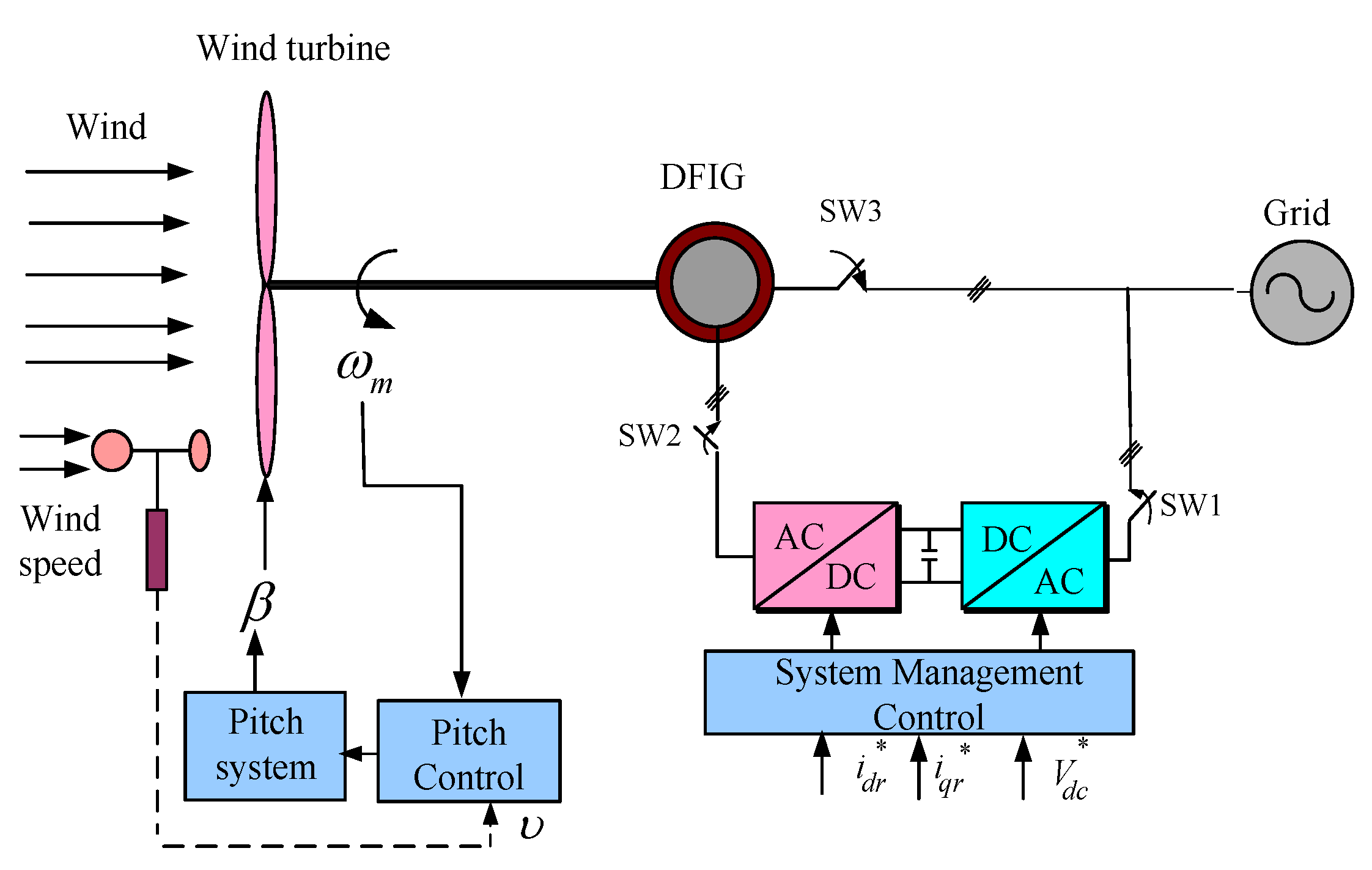
Conventional grid-connected DFIG topologies use a back-to-back converter in the rotor circuit and the stator is connected directly to the grid, as depicted in
Figure 1. The back-to-back converter consists of a rotor-side converter (RSC) and a grid-side converter (GSC). The RSC provides a magnetizing current to the rotor windings and controls both active and reactive power at the stator terminals. Furthermore, the RSC controls the stator active power to extract the maximum possible power from wind and enhance power quality through harmonic current filtering [
6,
7,
8,
9]. The RSC is also used to smooth stator synchronization with the grid in a zero current connection and a negligible effect to the supply and the generator. Moreover, the RSC should be designed to fulfil the grid code requirements to minimize the connection currents on the net connecting point. The main function of the GSC is to maintain a constant DC link voltage, regardless of power flow direction, and to control the magnitude and direction of rotor reactive power. The GSC is also used to remove reactive power pulsation under unbalanced conditions [
10,
11,
12].
Power converter performance largely depends on the accuracy of the implemented control strategy. Therefore, converter current controller performance is one of the most critical issues in power electronics circuits. The quality of a current controller can be evaluated based on several basic requirements [
13]:
Over a wide output frequency range, both phase and amplitude errors should be zero.
The controller should have a fast-dynamic response.
The effects of load parameters changes should be compensated for.
Constant or limited switching frequencies should ensure reasonable lifetimes for power electronics semiconductor devices.
Total harmonic distortion should be minimized.
The current controller techniques listed in the literature can be divided into two main categories [
14,
15,
16]: linear and nonlinear controllers. Proportional-integral (PI) stationary and synchronous, state feedback, and deadbeat controllers are examples of linear control techniques. These methods were introduced in [
17,
18].
The stationary PI technique has a major drawback in its inherent amplitude and phase error. To solve this problem and perform error compensation, several solutions have been proposed, such as using additional phase-locked loop (PLL) circuits [
19] or feedforward correction [
20]. However, when using asynchronous PI controller, the fundamental component error can be regulated to zero [
20], but dynamic properties are still an issue.
Another well-known controller, namely, the deadbeat controller, was designed to ensure strong dynamic responses [
21]. The main advantages of this controller are that voltage measurements are not required to generate current references [
22]. However, this controller suffers from a serious drawback in the form of inherent delays due to calculations. Furthermore, this controller does not include an integral control, which introduces steady-state errors.
The nonlinear controller category includes fuzzy logic controllers (FLC) and hysteresis controllers. A hysteresis current controller is typically implemented for the sake of simplicity. This method does not require any prior information regarding load parameters and has fast response. However, based on a fixed hysteresis band, this current controller has a narrow band of switching frequencies for minimizing the peak-to-peak current ripple at all points of the fundamental frequency wave [
23].
Another nonlinear controller, the FLC, is typically implemented as an alternative to a conventional PI compensator [
24,
25]. For this controller, the design steps and controller accuracy depend on the knowledge and experience of the user.
To compensate for these drawbacks, a state feedback controller working with stationary or synchronous rotating coordinates can replace a conventional PI controller. In this controller, a feedback gain matrix can be calculated to ensure sufficient damping. Furthermore, an integral component can be added to minimize steady-state error to zero. Reference and disturbance inputs are used as feedforward signals and then added to the feedback control law to reduce transient error. The performance of the state feedback controller has been discussed in a few papers, which have indicated superior performance compared to conventional PI controllers.
Several articles have proposed methods by which to synchronize the DFIG to the grid. In [
26], stator-flux oriented control was applied to the RSC to control the active and reactive power of the stator individually. However, the idea of this paper is to start the DFIG as a motor and then reverse the operation to operate as a generator which leads to a large inrush current with low power factor. In [
27,
28], a generated induced stator voltage is adjusted to be equal to the grid voltage by controlling the rotor flux. These articles guarantee a zero current connection which has no effect on both the generator and the grid. However, these studies proposed a synchronization process with the PI controllers which are used to control the magnitude and angle of the stator voltage. However, using such consecutive PI controllers slows the dynamic response and deteriorate the overall controller performance.
The proposed synchronization method can be implemented at any wind speed between the cut-in and cut-out speed and at any rotating speed of the wind turbine quickly and smoothly. This feature is very important during the grid faults such as voltage dips when the wind generation system is disconnected by the protective relays from the grid. The proposed method guarantees a fast and soft reconnecting of the system at any speed and with null current. To guarantee fast and smooth synchronization, state feedback current controllers are proposed to replace the PI current controllers for both converters. To demonstrate the validity and exceptional performance of the proposed control algorithm, an experimental setup was designed and implemented. Finally, a comparison between the proposed method and a PI controller in the synchronization process is presented.
2. System Description
In DFIG-based WECSs, when ignoring the stator core and copper losses, all active and reactive power is supplied by both the stator and rotor. A maximum power point tracker is typically implemented to maximize the stator active power, which is extracted from the wind turbine. Regarding the rotor rotational speed, rotor power can be either supplied to or drawn from the grid depending on the operating speed. The grid feeds the rotor when the rotor rotates at sub-synchronous speeds and the rotor current lags behind the rotor voltage by less than 90°. At super-synchronous speeds, the rotor windings feed power to the grid and the rotor voltage jumps to nearly 180° ahead of the stator voltage, where the slip value is negative [
29,
30,
31].
2.1. DFIG Model
DFIG equations are similar to those for a squirrel-cage induction generator. The only modification to the equations is that the DFIG rotor terminals are not short-circuited. DFIG characteristic equations can be derived from the equivalent circuit in a synchronously rotating direct quadrature (dq) frame, as shown in [
32].
The DFIG equations can be represented in a Park frame by the following equations [
32]:
where
: Magnetizing inductance;
: Stator self-inductance;
: Rotor self-inductance;
: Stator resistance;
: Rotor resistance;
: Stator dq-axis flux linkage;
: Rotor dq-axis flux linkage;
Synchronous and slip speed;
: Stator and rotor dq-axis currents;
: Stator and rotor dq-axis voltages.
In the case of stator-flux-oriented control, the d-axis is aligned with the flux vector. Therefore, the q-axis flux is zero and the main flux is the d-axis component.
The stator flux angle
is calculated from the flux components of the stationary coordinate system as follows:
where the superscript ‘s’ refers to the stationary coordinate system.
If the stator resistance is negligibly small, Equation (1) can be rewritten to calculate the stator d-axis flux as
The d- and q-axis components of the rotor flux equations can be determined from the stator flux and currents where the stator voltage vector is aligned with the q axis, which means it advances the stator flux vector by 90°. Then, the stator voltage is expressed as
As a result of Equations (3) to (6), the stator current components can be written as
and d-axis current is as follow:
By ignoring the power losses, the active power can be expressed as a function the d- and q-axis stator voltages and currents as follows:
Because the voltage d-axis component is zero, controlling the q-axis component of the rotor current controls the injected stator active power to the grid as
The reactive power can be controlled by adjusting the rotor D-axis current as
If the magnitude of the magnetizing current is kept constant, then the active and reactive power can be controlled linearly by regulating both the d- and q-axis currents. The control procedure for the RSC and GSC is detailed in the following section.
2.2. Rotor-Side Control
The power extracted from the wind at any wind speed and turbine rotational speed is calculated as follows [
33]:
where
: standard air specific density [kg/m3];
: power coefficient;
: pitch angle of the turbine blades [degrees];
: wind speed [m/s];
: tip-speed ratio (TSR);
: blade radius [m].
Figure 2 presents the turbine blade’s power variation with wind speed and rotational speed. The maximum power output occurs at a particular rotational speed.
The maximum power is defined as
This condition occurs when Cpmax is the maximum tip-speed-ratio is equal to which largely depends on the blade design.
The relationship between the turbine power and generator output power is calculated as
where
Pe is the generator electrical power,
J is the system moment of inertia,
Bt is the friction coefficient, and
is the blade rotational speed.
By substituting the maximum power from (13) into (14), the DFIG maximum generated power
Pe, max at each time step can be calculated as follows [
34]:
where
is the turbine speed that corresponds to the maximum mechanical power. By ignoring the generator iron and copper losses, the maximum stator active power
Ps, max can be calculated as [
35]:
The calculated from (16) is then used by the RSC controller to determine the optimal rotational speed as a stator active power reference (i.e., ) for maximum power point tracking.
By calculating the stator active power, the control block diagram of the stator power is presented in
Figure 3a. The PI controller gains for the active and reactive power controllers are
Kpp,
Kip,
Kpq, and
Kiq; respectively. The rotor reference q-axis current
is then calculated as the output of the active power controller and input for the inner current control loop. The rotor instantaneous q-axis current is then calculated from the sensed three-phase rotor currents and controlled to produce a reference q-axis rotor voltage. Normally, the output reactive power of the wind power conversion system is controlled as zero to keep unity power factor of the stator voltage and current. The stator reactive power is controlled to the desired value to produce the reference d-axis rotor voltage as shown in
Figure 3b. One can see how the outer stator power feedback loop produces the rotor reference d-axis current
for the inner current feedback control loop. The reference q-axis rotor voltage is then produced by controlling the rotor d-axis component.
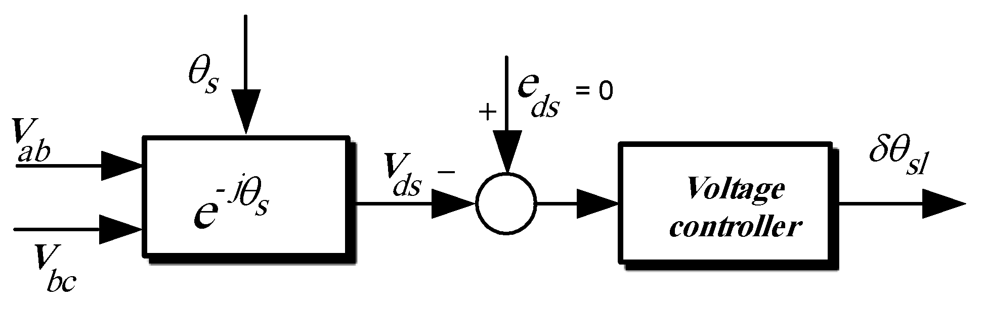
However, the DFIG synchronization mode control is different from the power mode control. To synchronize the DFIG with the grid, smooth connection of the DFIG to the grid is achieved when the stator voltage amplitude, frequency and phase are equal to the grid voltage before closing the switch between the stator and the grid. The rotor side controller is activated to calculate the excitation current for the grid synchronization and power control loops. The excitation current generates the generator flux which builds-up the stator terminal voltages while the turbine accelerates until it reaches a certain value (e.g., 80% of the rated speed). At the same moment, the dc-link voltage in the bidirectional converter is soon charged. In addition, the stator frequency is almost the same as the grid, and the stator voltage amplitude is also the same as that of the grid. Even slightly different frequencies may cause the phase difference between the two voltages. To compensate the phase difference between the stator EMF
νds and grid voltage, the phase difference compensation component
is added to the calculated slip angle as shown in
Figure 4 [
36]. The compensation component
is calculated by controlling the stator d-axis voltage component to be zero, equal to the grid d-axis voltage.
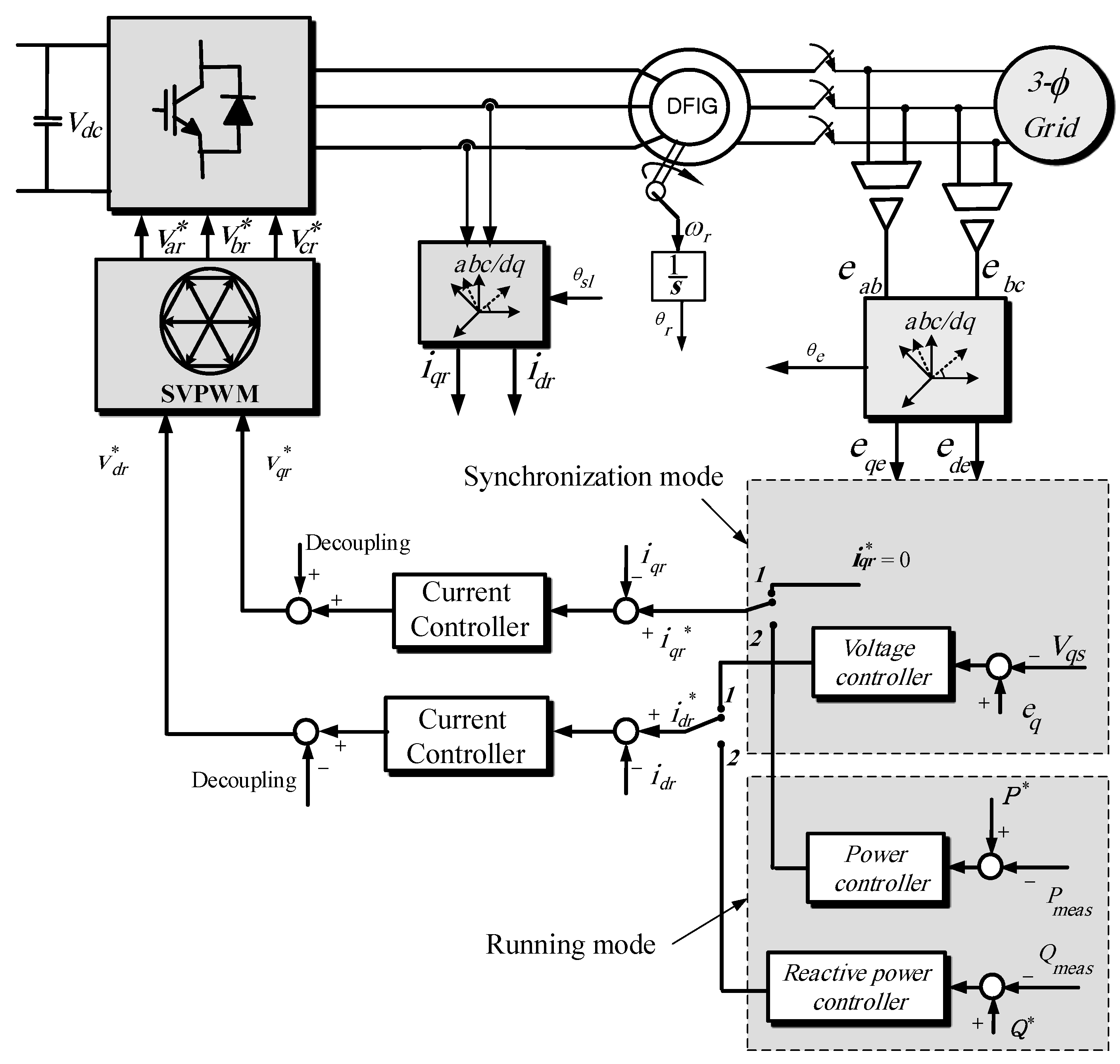
Once this process has been accomplished, the stator-side contactor is closed, and the generator is connected to the grid and then the power control mode starts. The generator power reference is set to the maximum value and the system is fully integrated to the grid. The sequence of synchronization is shown in
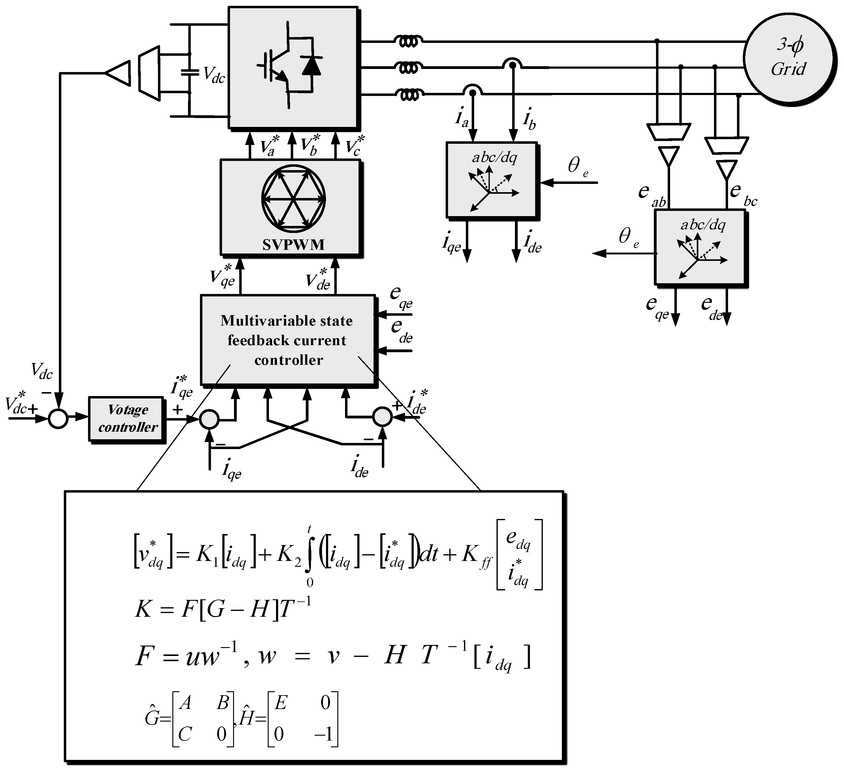
Figure 5 and the overall control system for both synchronization mode and running mode is shown in
Figure 6. The grid voltages
eab and
ebc are measured and transformed to dq-axis components
eds and
eqs; respectively. Similarly, the rotor currents
iar and
ibr are measured and used to obtain the dq-axis currents which are
idr and
iqr; respectively.
and
are the reference rotor dq-axis voltages, while
,
and
are the RSC reference voltages.
3. Grid-Side Multivariable State Feedback Control
The goal of the GSC is to maintain a constant DC link voltage and boost it to a level that is higher than the amplitude of the line-line voltage. The DC link voltage is regulated to the reference value by using a PI controller. Any variation in the DC link voltage causes a change in the Q-axis reference current. The reactive power (or power factor) is controlled by using the D-axis reference current.
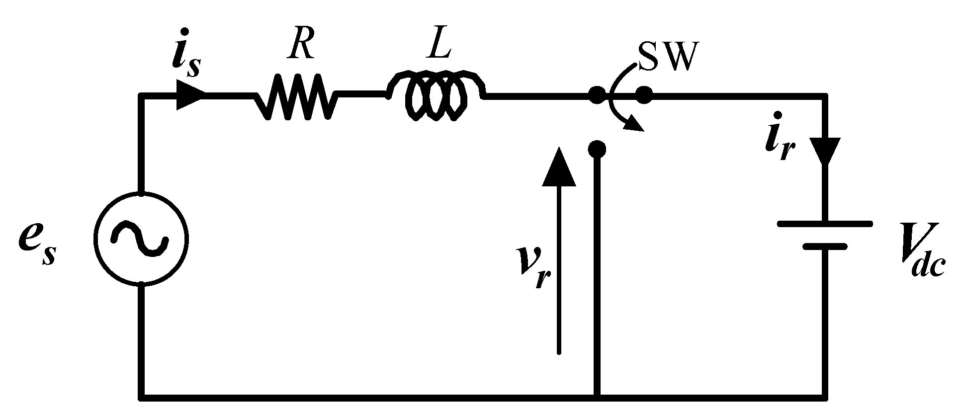
Figure 7 presents the voltage source-pulse width modulation (VS-PWM) converter equivalent circuit for each phase. The circuit voltage equation can be derived from the figure as [
37]
where,
A state-space model for the converter can be obtained by expressing (17) in a synchronous frame as
where,
x: state vector;
: derivative of the space vector with respect to time;
u: input or control vector;
d: input disturbance vector;
y: output vector;
A: system matrix;
B: input matrix;
C: output matrix;
E: disturbance matrix.
Additionally,
and ω is the angular frequency of the source. The state variables
x are the source currents, the input vectors
u are the converter input voltages in the DQ axis, the disturbance
d is the source voltage in the DQ axis, and the output
y is the equal to source current.
3.1. State Feedback Control
Equations (18) and (19) define the state space model for any time-invariant linear multivariable system. When
, the control target is [
38,
39]
where
yr is a reference output.
Because state feedback control is known to be a type of proportional control, the system performance in a steady state is inaccurate based on model uncertainty. This disadvantage can be overcome by introducing an integral control function to minimize steady-state error. The integral control function for the error
p is defined as
Assuming that the reference output and disturbances are constant, substituting the derivative of (20) into (17) yields the following differential equations:
By transforming these equations into matrix form, an augmented state model can be expressed as
In a steady state, the derivatives of the space vector and error approach zero because the disturbances and output references are assumed to be constant. Therefore, the steady-state solutions
,
, and
, where the subscript “s” denotes a steady-state value, must satisfy the following equation:
Substituting (23) into (22) yields
To represent the deviations in these solutions from the steady state, a definition for new variables is introduced as follows:
Equation (29) can be defined in the standard state space equation as follows:
where
The system in (27) is controllable when linear state feedback control can be applied. In such cases, the system can be expressed as follows:
where
The partitioned matrices are derived via pole placement. By substituting from (24), (25), and (28), the control law is obtained as
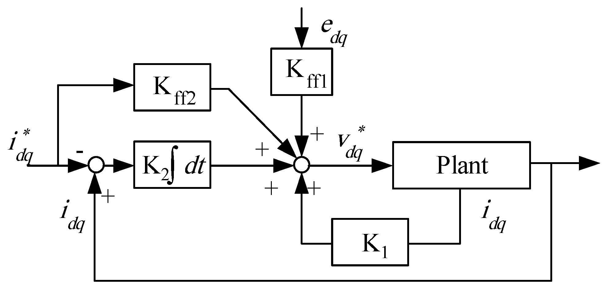
3.2. Feedforward Control
By using an integral controller, static errors can be regulated to be zero. However, system dynamic errors may be large during transients and disturbances. To reduce transient errors and the effect of disturbances, feedforward control can be used. To derive feedforward control equations, both reference inputs and disturbance inputs are used. The deviation of the output from the reference can be calculated as
The control system can be defined based on (18), (19), and (30) as follows:
The left-hand side of (31) becomes zero when the steady state reaches the steady-state condition. In this case,
where
Now, deviations from the steady state can be expressed using new variables as
By substituting (33) into (32), we get
The new relationship is the same and is defined as
By substituting (32) into (35), we get
where the feedforward gain is defined as
The state variables, disturbances, and reference input equations comprise the total control equation, which is derived by substituting the integral control equation (20) into (36). The resulting control equation is written as follows:
To illustrate the total control law in (37), a block diagram for the current controller, including the feedback and feedforward components, is presented in
Figure 8.
3.3. Pole placement technique
A pole placement method is used to obtain the feedback and feedforward gain matrices for (37) by using the generalized control conical form (GCCF). The open-loop system equation is defined as follows:
where
x is a vector of size
n × 1,
A is a gain matrix of size
n ×
m, u is a vector of size
m × 1, and the dimension of the gain
B is
m. This equation can be transformed into the GCCF through the transformations described below.
where
and is the controller variable gain with a rank equal to u.
and
are matrices of rank
and
, respectively, and have the forms
To derive the GCCF in (40), three transformations can be performed on (39):
The ranks of H and
v are
m x
m and
m x 1, respectively. Substituting the matrix
w from (46) into (45) yields
The
T, T−1, F, and
H matrices are required to calculate the gains. The multivariable system controllability matrix can be defined as
Inverting (48) yields (49):
where
and
i = 1, 2,…,
m. The bottom row of each partitioned submatrix
is used to form a transformation matrix
T–1 of the form
T is calculated by taking the inverse of (31). F is derived from (44) and H is derived from (46).
The state feedback control is applied as
Ad is a closed-loop matrix that can be written as
A formal expression for
can be obtained because
This leads to the expression
By returning to the original state space,
where
.
The feedback and feedforward controller components are depicted in
Figure 9. The controller gain,
K = [0.0075, 5.2].
The actual DC link voltage is measured and compared to the voltage reference . The difference signal is then minimized by the DC link voltage controller. The output of the controller produces an inverter current reference and . The grid voltages and three-phase line currents are sensed and transformed into d- and q-frame axes. The dq currents and voltages are then used in conjunction with the state feedback matrix (56) to develop feedback voltage reference components. Similarly, both the source voltage and reference currents from the d and q axis components are combined with the feedforward gain matrix in (37) to develop the feedforward components of the inverter input voltage reference, which are then transformed and used to modulate the inverter.
4. Experimental Results
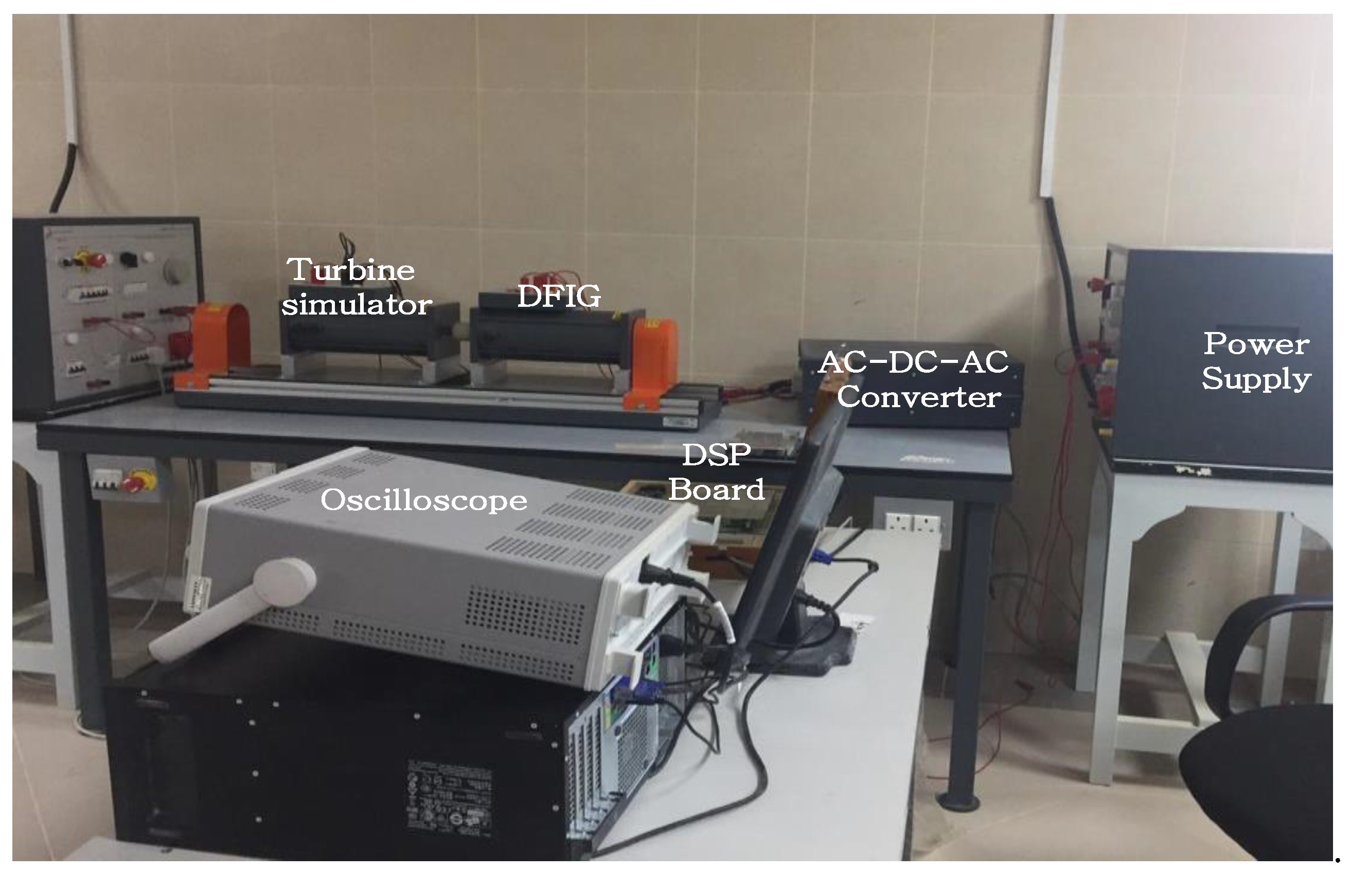
Experiments were performed to study the performance of the multivariable state controller separately from the DFIG system. Several tests of the real operation of an insulated gate bipolar transistor (IGBT)-based PWM inverter in different conditions were conducted. It is desirable for the WECS to be implemented with hardware (motor-generator set) to test system operations in a laboratory.
Figure 10 presents the experimental setup in the laboratory, which consists of a DFIG driven by a wind simulator, back-to-back converters, and digital signal processor (DSP) TMS320C33 control boards. The parameters of the wind turbine and DFIG can be found in
Appendix A.
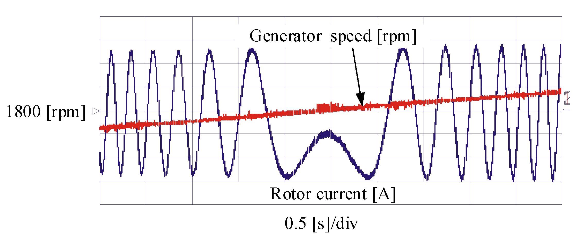
The synchronization process starts by accelerating the wind turbine simulator which is mechanically coupled with the DFIG. This step may take long time depends on the system inertia. During the acceleration, the DC-link capacitor is charged through the GSC. After the DC-link is charged, the rotor state feedback dq current controllers are started to build up the stator voltage. After inducing the stator voltage, it is necessary to synchronize the stator to the grid, which is applicable at any rotating speed when the stator terminals are open. The electromagnetic torque is zero in this stage. The switch between stator terminals and grid is switched on when the stator and grid voltages are equal in amplitude and frequency.
Figure 11 shows the rotor current variation from sub to super-synchronous speed. It is clear that the speed varies from sub to super-synchronous smoothly when a back-to-back converter is used. As the rotor speed increases, the rotor power decreases to zero and increases in the reverse direction. Theoretically, the rotor power reverses its direction at a synchronous speed. However, the zero-crossing doesn’t occur at the synchronous speed due to the different system losses such as rotor and converter losses.
4.1. Synchronization Assessment
To connect the DFIG with the grid, the grid-side controller synchronizes the stator and grid voltages by building up the stator voltage by controlling the rotor d-axis current. The phase shift between the two voltages is compensated for by using the proposed PLL algorithm. This synchronization process takes place in a nearly coupled cycle.
The synchronization process is depicted in
Figure 8, when the stator voltage is synchronized with the grid voltage.
Figure 12a shows the connection process of a certain phase voltage of stator voltages with the corresponding phase of grid voltage. From zero stator voltage, the rotor d-axis current is controlled in order to build up the stator voltage in a short time. Meanwhile, the phase shift between the two voltages is compensated as shown in
Figure 12b. This process takes place in an almost one cycle. To demonstrate the superiority of state feedback over PI controller, the synchronization process is performed as shown in
Figure 13. The synchronization takes about two cycles, which is twice the synchronization time of the proposed method.
4.2. Power Control Mode
In
Figure 14, the controller performance is investigated during a periodic speed variation. The minimum and maximum values are respectively 6 m/s and 8 m/s; respectively. In the power optimization region (at low wind speeds less than 12 m/s), the pitch angle controller is passive, keeping the pitch angle constant to the optimal value which is zero for the considered wind turbine. Meanwhile, the power controller controls the active power to the active power reference value provided by the maximum power tracker. Thus, the active power follows the wind speed pattern as shown in
Figure 14b. Meanwhile, the rotor q-axis current component and generator torque follow the same pattern as shown in
Figure 14c,d. To maintain the output power factor to unity, the reactive is adjusted to zero and the d-axis current remains constant as shown in
Figure 14e,f.
Figure 15 presents the controller performance with step changes in wind speed. The wind speed increases in increments of 2 [m/s], starting from 5 [m/s]. For wind speeds less than 12 m/s, the pitch angle controller does not operate because the pitch angle is zero for the considered wind turbine. The power controller controls the real power component to extract the maximum possible power.
The power controller response at lower wind speeds is faster than the response at higher wind speeds. At wind speeds higher than 12 m/s, the pitch angle controller begins to operate to reduce the stress on the turbine blades.
Next, the stochastic nature of real wind speeds has been simulated.
Figure 16 presents the DFIG parameters under turbulent wind speeds, where the mean wind speed is 10 m/s and the turbulence intensity is 20%. The active power changes when the wind speeds lower than 10 m/s, but it is maintained at the rated value when the wind speed increases beyond the rated value.
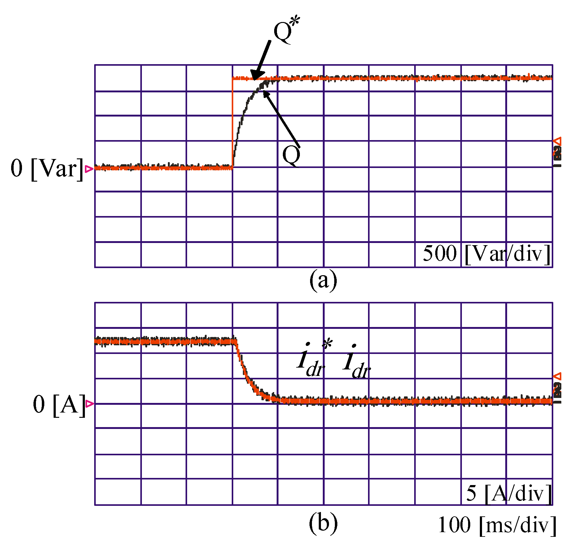
To test the proposed controller performance, the stator reactive power reference was changed in a step from 0 to 1750 Var, as shown in
Figure 17. The actual reactive power follows the changes and the rotor d-axis current follows the reference as shown in
Figure 17a,b. The measured stator and rotor currents are depicted in
Figure 18a,b. It is obvious that the currents are almost sinusoidal.
4.3. GSC Controller Assessment
To investigate the performance of the inverter separately, the terminals were connected to a variable load. For the case of a step change in the inverter load,
Figure 19 and
Figure 20 present the DC link voltage, and d- and q-axis current transient responses. From these figures, one can see that the transient responses from the two controllers are nearly the same, except that the overshoot in the q-axis current of the PI controller is slightly larger than that of the multivariable state feedback control. Furthermore, the performance of the latter controller is satisfactory in both transient and steady states.
Finally, the root mean square error (RMSE) for the rotor quadrature axis current in case of PI and state feedback controller, since this component controls the stator active power.
Table 1 shows RMSE values which demonstrate a very small difference between the two controllers.
To test the validity of state feedback controllers when a unbalanced grid-voltage occurs, the amplitude of phase voltages
and
are reduced to produce unbalanced grid voltage as shown in
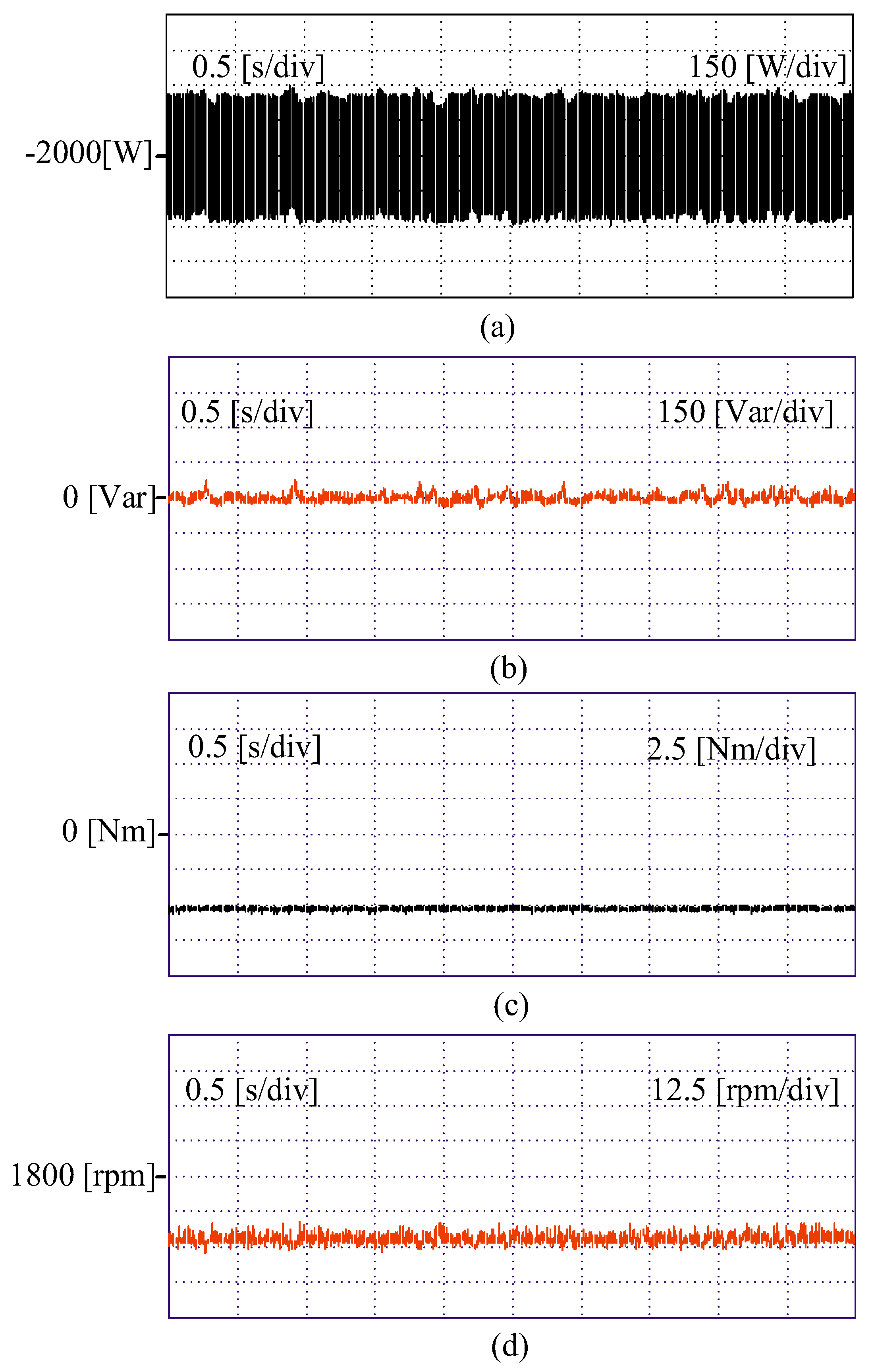
Figure 21. The unbalanced rotor currents are analysed to the positive and negative sequence components. Four state feedback current controllers are used to control the dq-axis positive and negative rotor currents. The main objective of these controllers is to regulate the stator active and reactive power in the pre-determined level by regulating the rotor positive sequence dq-axis components. Meanwhile, the rotor negative sequence dq-axis current components are controlled to eliminate the generator torque pulsation.
Figure 22a shows the active power waveform when the reactive power ripples are controlled. The active power has large amount or pulsations around the reference value which is 2kW.
Figure 22b shows the reactive power of the stator with an average value of 0 and no pulsation.
Figure 22c shows the generator torque at this time and the pulsation component is very small. The generator speed oscillations decreased for about 0.25 [rpm] due to torque pulsation reduction in
Figure 22d. Therefore, in order to reduce the torque ripple of the DFIG when unbalanced grid-voltage occurs, the stator reactive power pulsations should be eliminated.

 ,
, 


