DNN-Assisted Cooperative Localization in Vehicular Networks

Abstract

This work develops a deep-learning-based cooperative localization technique for high localization accuracy and real-time operation in vehicular networks. In cooperative localization, the noisy observation of the pairwise distance and the angle between vehicles causes nonlinear optimization problems. To handle such a nonlinear optimization task at each vehicle, a deep neural network (DNN) technique is to replace a cumbersome solution of nonlinear optimization along with the saving of the computational loads. Simulation results demonstrate that the proposed technique attains some performance gain in localization accuracy and computational complexity as compared to existing cooperative localization techniques.

1. Introduction

As vehicular networks, in which the internet of vehicle (IoV) technology is considered, have been developed, a localization technique for accurate positioning is demanded. Most of well-known vehicle localization techniques resort to global navigation satellite systems (GNSS). However, it is also known that GNSS itself is not sufficient for autonomous driving for its limited accuracy and availability in urban and indoor areas [1]. To localize the vehicle when the GNSS signal is blocked, there have been a number of localization techniques [2,3] that mostly require the distance and angle from the base station. In addition, several cooperative localization techniques are additionally developed [4,5]. In [4], the extended Kalman filter with the information graph is applied to carry out the location estimation in a round robin manner with geolocation information of round trip time (RTT) from the received signal. The sum–product algorithm [6,7] over a wireless network (SPAWN) is developed for calculating the marginal posterior distribution of the position of a target node [5]. Although such a Bayesian-based cooperation attains high localization accuracy, it also poses several challenges regarding the computational complexity in calculating and representing the posterior distributions.

For solving the complexity problem, a variety of algorithms [8,9,10,11] are developed with the assumption that the propagated probability distribution is Gaussian, but high non-linearity of the angle measurement is not considered. Very recently, an optimization technique based on an alternating direction multiplier method was developed [12] for further saving of computational efforts in cooperation. In addition, the connectivity among vehicles enhances the performance of the message-passing-based cooperative localization algorithm [13]. However, when it comes to simultaneous consideration of computational complexity saving and performance improvement, a number of technical challenges still remain.

During the past decade, deep learning technology has become a promising alternative to handle complicated technical tasks in various applications [14,15]. Furthermore, the use of deep learning in wireless communication in vehicular networks began to appear recently [16,17,18,19]. In [16], deep learning proves promising in MIMO, femtocell, and device-to-device (D2D) technologies with the upcoming deployment of the 5G network. Also, a success in land detection and driving assistance in vehicular networks has been made via a deep learning technique [18]. Along with various applications in vehicular networks [20,21,22], the localization in IoV network is not an exception. A fingerprinting technique for online positioning through received signal strength intensity (RSSI) data collection of location information offline is applied to deep learning localization [23,24]. A method which classifies a position matched with RSSI data using a deep neural network (DNN) is used. Deep learning is also applied to classify the LoS/NLoS of the communication signal to improve localization accuracy [25].

In this paper, we develop the deep-neural network (DNN) technique to mitigate the computational complexity while sustaining the localization accuracy. For training the DNN, we design geometric measurements between two vehicles and relative locations of the vehicle as the input data and the output data, respectively. The structural similarity between DNN and cooperative localization in that nonlinear objective is decomposed into various sets of hidden layers [20], which enables the DNN to tackle the non-linearity in the localization function. This work elaborates a cooperation approach of incorporating the DNN technique with the proposed cooperative localization challenge. The DNN enables us to solve a chronic nonlinear approximation problem, and enhance the computational complexity. The DNN-assisted relative localization is then combined in a round robin manner to cooperatively localize all the vehicles in the networks. We demonstrate that the proposed DNN technique improves localization accuracy and also complexity of cooperative localization in the vehicular network.

2. Problem Formulation

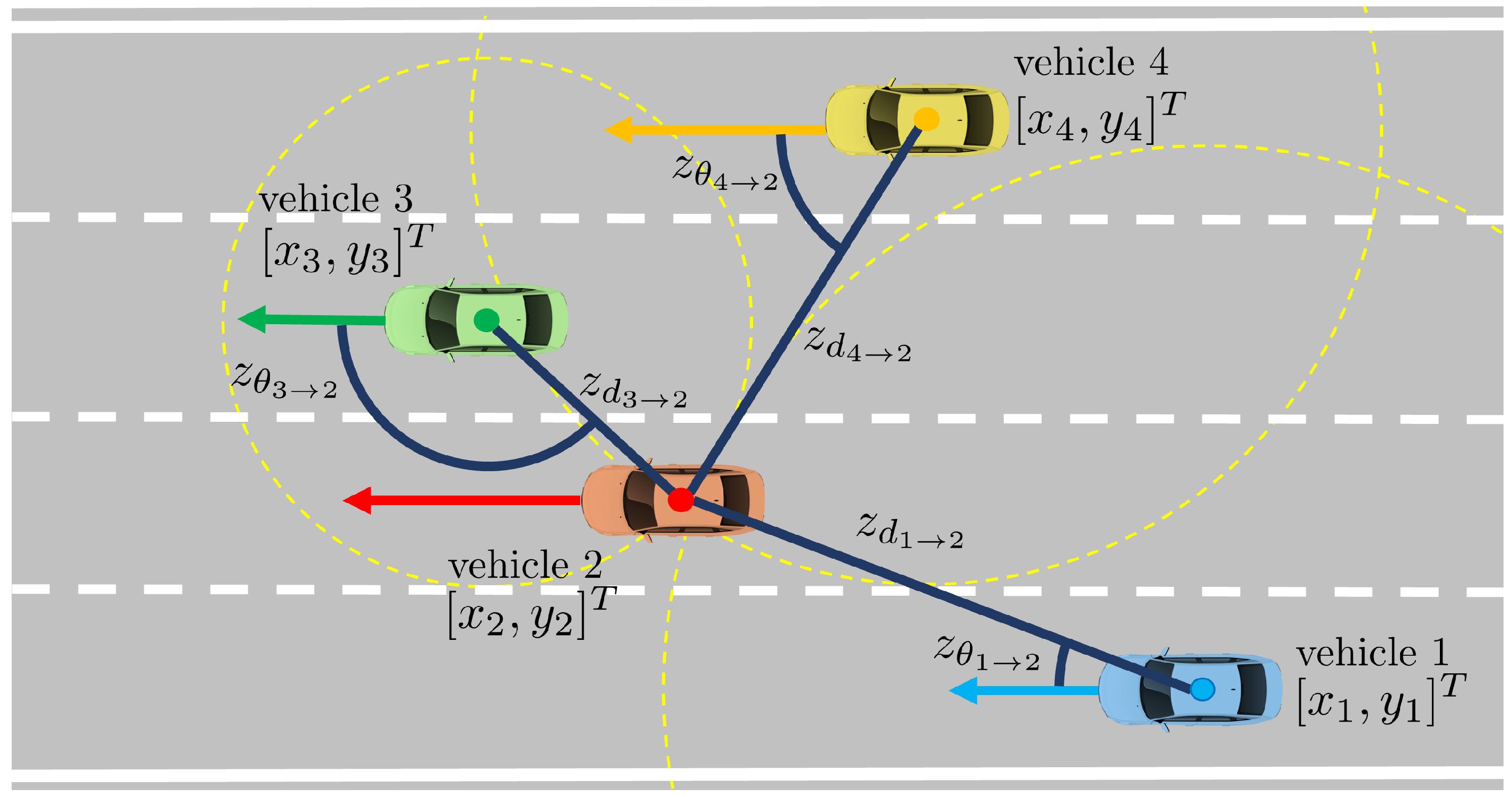
We consider a two dimensional vehicular network, where I vehicles are deployed. It is assumed that all vehicles communicate with each other, so that all vehicles are connected via peer-to-peer fashion. Let us also assume that the vehicle observes the distance and angle of arrival (AoA) from its neighboring vehicles within the range of $d_{\mathrm{range}}$, and the distance and AoA measurements are provided by the sensor on the board of the vehicle. There is no data fusion center which collects the measurements from distributed vehicles and calculates location of each vehicle. The vehicle gathers measurements from other vehicles, and then cooperatively estimates own location. Here, $d_{\mathrm{range}}$ indicates maximum range that the distance and angle sensing is possible. In our vehicular network, the vehicle index i and j indicate the target and its neighbors, respectively. The location of the i-th vehicle is denoted by ${\mathbf{x}}_i={[x_i,y_i]}^{\mathrm{T}}$, and the location of the j-th vehicle is represented in a similar notation. The pairwise distance between the i-th and j-th vehicle is given by $d_{i,j}={|{\mathbf{x}}_i-{\mathbf{x}}_j|}^2$. The AoA at the i-th to j-th vehicle is given by ${\theta }_{i\to j}=arctan\{(y_j-y_i)/(x_j-x_i)\}.$ In addition, a set containing the indices of neighboring vehicles connected to the i-th vehicle is denoted by ${\mathbf{N}}_i$. The pairwise distance at the i-th to j-th vehicle [26] that undergoes the measurement noise is denoted by $z_{d_{i\to j}}=d_{i,j}+n_{d_{i,j}}$ where the distance measurement noise $n_{d_{i,j}}$ is a zero-mean Gaussian random variable with standard deviation ${\sigma }_{d_{i,j}}=(d_{i,j}/d_{\mathrm{range}}){\sigma }_d$ [27]. The distance measurement error becomes larger as the distance between the vehicles increases. The AoA is measured by determining the direction of the propagation of an incoming radio frequency wave. When all vehicles are connected via peer-to-peer manner, then all vehicles observe the measurement its neighboring vehicles. Figure 1 represents the vehicular network where 4 vehicles are deployed, and vehicle 2 observes distance and angle measurements from neighboring vehicles. The corresponding AoA at the i-th to the j-th vehicle is given by $z_{{\theta }_{i\to j}}={\theta }_{i\to j}+n_{\theta }$, where the AoA measurement noise $n_{\theta }$ is zero-mean Gaussian random variable with standard deviation ${\sigma }_{\theta }$. Given the distance and AoA measurements, likelihood functions $p\left(z_{d_{i\to j}}\right|{\mathbf{x}}_i,{\mathbf{x}}_j)$ and $p\left(z_{{\theta }_{i\to j}}\right|{\mathbf{x}}_i,{\mathbf{x}}_j)$ corresponding to measurements are easily derived as

$$\begin{array}{c}\hfill p\left(z_{d_{i\to j}}\right|{\mathbf{x}}_i,{\mathbf{x}}_j)=\frac{1}{\sqrt{2\pi {{\sigma }_d}^2}}exp\left\{-\frac{|z_{d_{i\to j}}-d_{i,j}{|}^2}{2{\sigma }_d^2}\right\},\\ \hfill p\left(z_{{\theta }_{i\to j}}\right|{\mathbf{x}}_i,{\mathbf{x}}_j)=\frac{1}{\sqrt{2\pi {{\sigma }_{\theta }}^2}}exp\left\{-\frac{|z_{{\theta }_{i\to j}}-{\theta }_{i\to j}{|}^2}{2{\sigma }_{\theta }^2}\right\},\end{array}$$

(1)

with distance likelihood function and AoA likelihood function, the relative likelihood function between two vehicles can be derived as

$$p\left({\mathbf{z}}_{i\to j}\right|{\mathbf{x}}_i,{\mathbf{x}}_j)\propto p\left(z_{d_{i\to j}}\right|{\mathbf{x}}_i,{\mathbf{x}}_j)p\left(z_{{\theta }_{i\to j}}\right|{\mathbf{x}}_i,{\mathbf{x}}_j),$$

(2)

where ${\mathbf{z}}_{i\to j}$ is a 2 by 1 measurement vector consisting of $z_{d_{i\to j}}$ and $z_{{\theta }_{i\to j}}$. Although the information of the relative location can be calculated in this way, it is inefficient to compute with likelihood functions between the vehicles due to the noise included in the measurement causes the high complexity issues [13].

Given all measurements $\mathbf{z}$ consisting of ${\mathbf{z}}_{i\to j}\forall i,j$ on all vehicle locations $\mathbf{x}=[{\mathbf{x}}_1,\dots ,{\mathbf{x}}_I]$ and the prior distribution $p\left(\mathbf{x}\right)={\prod }_{i=1}^{I}p\left({\mathbf{x}}_i\right)$, the well known posterior distribution $p\left(\mathbf{x}\right|\mathbf{z})$ is factorized as

$$p\left(\mathbf{x}\right|\mathbf{z})\propto \prod _{i=1}^{I}p\left({\mathbf{x}}_i\right)\prod _{j=1}^{N_i}p\left({\mathbf{z}}_{i\to j}\right|{\mathbf{x}}_i,{\mathbf{x}}_j).$$

(3)

The vehicle location is estimated by the minimum mean square error or maximum a posterior estimator from the marginal posterior distribution. The marginal posterior distribution for the i-th vehicle is calculated as

$$p\left({\mathbf{x}}_i\right|\mathbf{z})\propto p\left({\mathbf{x}}_i\right)\int \prod _{j=1}^{N_i}p\left({\mathbf{x}}_j\right)p\left({\mathbf{z}}_{i\to j}\right|{\mathbf{x}}_i,{\mathbf{x}}_j)d\sim \left\{{\mathbf{x}}_i\right\},$$

(4)

where $\sim \left\{{\mathbf{x}}_i\right\}$ is defined as integration over all variables except for ${\mathbf{x}}_i$. However, the calculation of the marginal posterior distribution has implementation issues of the high computational complexity regarding the localization accuracy or linear/Gaussian assumption of system regarding the complexity. Considering the non-linearity/non-convexity of the likelihood function, it is trivial that one of the challenges in cooperative localization is a measurement update. Thus, we employ the DNN technique to overcome complexity issue, and the measurement update step (i.e., propagating the marginalized message) is replaced with the DNN.

3. Deep Learning-Based Approach in Cooperative Localization

3.1. DNN Architecture

To overcome the real-time implementation problem of cooperative localization, we choose the DNN technique for our learning model which is one of the most commonly used supervised learning methods. Our DNN model replaces the measurement update in our vehicular network and alleviates the complexity of the algorithm. The proposed DNN system is pre-trained with a combination set of input and output data related to the noisy measurement model. DNN architecture provides DNN structure (consisting of input, output, and hidden layers), a size of DNN structure [28]. Datasets are imported in the input and output layer for training the DNN [29], and details of dataset generation will be dealt in Section 4.1. The linear regression model is selected for each layer, and they are fully connected. The input layer consists of two nodes which are $z_{d_{i\to j}}$ and $z_{{\theta }_{i\to j}}$, and the output layer consists of two nodes which are the x and y location of ${\tilde{\mathbf{x}}}_{j\to i}^l$, where ${\tilde{\mathbf{x}}}_{j\to i}^l$ is defined as an intermediate location estimate.

A ReLU function [29] is utilized as a activation functions, and a linear function [28] is adopted for output layers. The ReLU function is one of activation functions that defined as the positive part of its argument is $g\left(h\right)=max(0,h),$ where h is the input to a neuron. Convergence of the weight component in the DNN depends on the optimizer function. We choose an Adam optimizer which operates to function to control the component of weight vector [30]. The nonlinear function is represented by the hidden layer. The number of layers is set to three, and each hidden layer has 32 nodes.

We use the dropout and regularization method to prevent the overfitting problem [31]. Overfitting is a phenomenon in which the error of actual data is increased by over-learning the learning data. In general, the learning data is a subset of the actual data, and is difficult to solve because it is difficult to collect all of the actual data. Predicting coordinates through learning is less accurate due to this problem. Since estimating the location with deep learning has such inaccuracies, we applied dropout and regularization to predict untrained locations. For details of the parameters used in our DNN structure, refer to

Table 1. Hyperparameters of deep neural network (DNN).

Parameter	Value
Batch size	100
Learning rate $\alpha$	0.001
The number of hidden layers	3
The number of nodes at k-th hidden layer $H_k$	32
The number of nodes at input layer $L_{\mathrm{in}}$	2
The number of nodes at output layer $L_{\mathrm{out}}$	2
Regularization strength $\beta$	0.001
Activation Function	ReLU, Linear
Optimizer	Adam
epoch	10
Distance measurement error ${\sigma }_d$	1 m
AoA measurement error ${\sigma }_{\theta }$	1${}^{°}$

. The relative measurements between vehicles consist the dataset of DNN. The distance and AoA measurements acquired pass through the DNN, and the relative location of the vehicle is estimated. The model, which has used in the algorithm, is described in this paragraph, and hyperparameters in Table 1.

3.2. Algorithm Structure

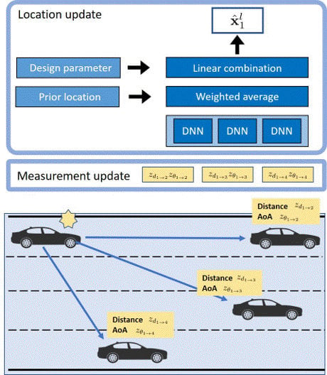
The following description introduces details of the cooperative localization algorithm with the proposed DNN dealt in the previous section. To solve the formulated problem (4), we adopt the iterative message passing intuition [12]. Figure 2 shows the scenario of the proposed algorithm which is performed over L iterations until the updated location converges.

Let the i-th vehicle variable initially take prior information $\sim \mathcal{N}({\widehat{\mathbf{x}}}_i^0,{\mathsf{\Sigma }}_0)$, where ${\mathsf{\Sigma }}_0$ is a diagonal matrix with identical diagonal entries ${\sigma }_0^2$. At the l-th iteration, vehicle variable node receives the message ${\tilde{\mathbf{x}}}_{j\to i}^l$ which is determined in the measurement update via DNN from neighboring factor nodes $j\in {\mathbf{N}}_i$. The message emanating from a variable node is calculated by equating all input messages, which correspond to minimizing the sum of squared error given by

$$\begin{array}{c}\hfill q\left({\widehat{\mathbf{x}}}_i^l\right)=\frac{\parallel {\widehat{\mathbf{x}}}_i^l-{\widehat{\mathbf{x}}}_i^0{\parallel }^2}{2det|{\mathsf{\Sigma }}_0|}+\sum _{j\in {\mathbf{N}}_i}\frac{\parallel {\widehat{\mathbf{x}}}_i^l-{\tilde{\mathbf{x}}}_{j\to i}^l{\parallel }^2}{2{\sigma }^2},\end{array}$$

(5)

where $\sigma$ is the square-root of the cost function for evaluating the data training in DNN. The cost function is defined as

$$\begin{array}{c}\hfill {\sigma }^2=\frac{1}{M}\sum _{m\in {\mathsf{\Omega }}_M}|{\overline{\mathbf{x}}}_m-{\mathbf{x}}_m{|}^2,\end{array}$$

(6)

where ${\mathbf{x}}_m$ is the m-th target data point, and ${\overline{\mathbf{x}}}_m$ is the output. M is the number of data points, and ${\mathsf{\Omega }}_M$ is a set of the data point. Since the function $q({\widehat{\mathbf{x}}}_i^l)$ is convex with respect to ${\widehat{\mathbf{x}}}_i^l$, the optimal value of ${\tilde{\mathbf{x}}}_i^l$ is calculated by solving a linear equation associated with the derivative of (5) equal to zero. The resulting ${\widehat{\mathbf{x}}}_i^l$ corresponding to the location estimate of the i-th vehicle is given by

$$\begin{array}{cc}\hfill {\widehat{\mathbf{x}}}_i^l=& \delta {\widehat{\mathbf{x}}}_i^{l-1}+(1-\delta )\left({\displaystyle \frac{{\displaystyle \frac{1}{det|{\mathsf{\Sigma }}_0|}}}{{\displaystyle \frac{1}{det|{\mathsf{\Sigma }}_0|}}+{\displaystyle \frac{I-1}{{\sigma }^2}}}}{\widehat{\mathbf{x}}}_i^0+\sum _{j\in {\mathbf{N}}_i}{\displaystyle \frac{{\displaystyle \frac{1}{{\sigma }^2}}}{{\displaystyle \frac{1}{det|{\mathsf{\Sigma }}_0|}}+{\displaystyle \frac{I-1}{{\sigma }^2}}}}{\tilde{\mathbf{x}}}_{j\to i}^l\right),\hfill \end{array}$$

(7)

where ${\mathbf{x}}_i^{l-1}$ is the up-to-date location at the previous iteration. Here, the updated message is obtained from a linear combination of the message at the previous iteration ${\widehat{\mathbf{x}}}_i^{l-1}$ and the message evaluated at the current iteration ${\tilde{\mathbf{x}}}_i^l$ with coefficients $\delta$ and $1-\delta$, respectively. Such a damping technique reduces the fluctuation of the updated messages at each iteration to improve the convergence of the algorithm. In every iteration, we consider the up-to-date location ${\tilde{\mathbf{x}}}_{j\to i}^l$ since each location is sequentially updated in a round-robin scheduling. The proposed algorithm is described in Algorithm 1.

Algorithm 1 Proposed cooperative localization via deep neural network (DNN).

1: given ${\widehat{\mathbf{x}}}_i^0,\forall i$   2: for$i=1$ to I do   3:     measure the relative distance $z_{d_{i\to j}}$ and AoA $z_{{\theta }_{i\to j}}$ to j-th vehicle, $\forall j\in {\mathbf{N}}_i$   4: end for   5: for$l=1$ to L do   6:     for $i=1$ to I do   7:         receive the up-to-date location of neighbor vehicles, $\forall j\in {\mathbf{N}}_i$   8:         obtain the intermediate location of the i-th vehicle relative to j-th vehicle ${\tilde{\mathbf{x}}}_{j\to i}^l$ with DNN, $\forall j\in {\mathbf{N}}_i$   9:         update location estimate using (7). 10:     end for 11: end for

4. Simulation and Discussions

4.1. Dataset for Training the DNN

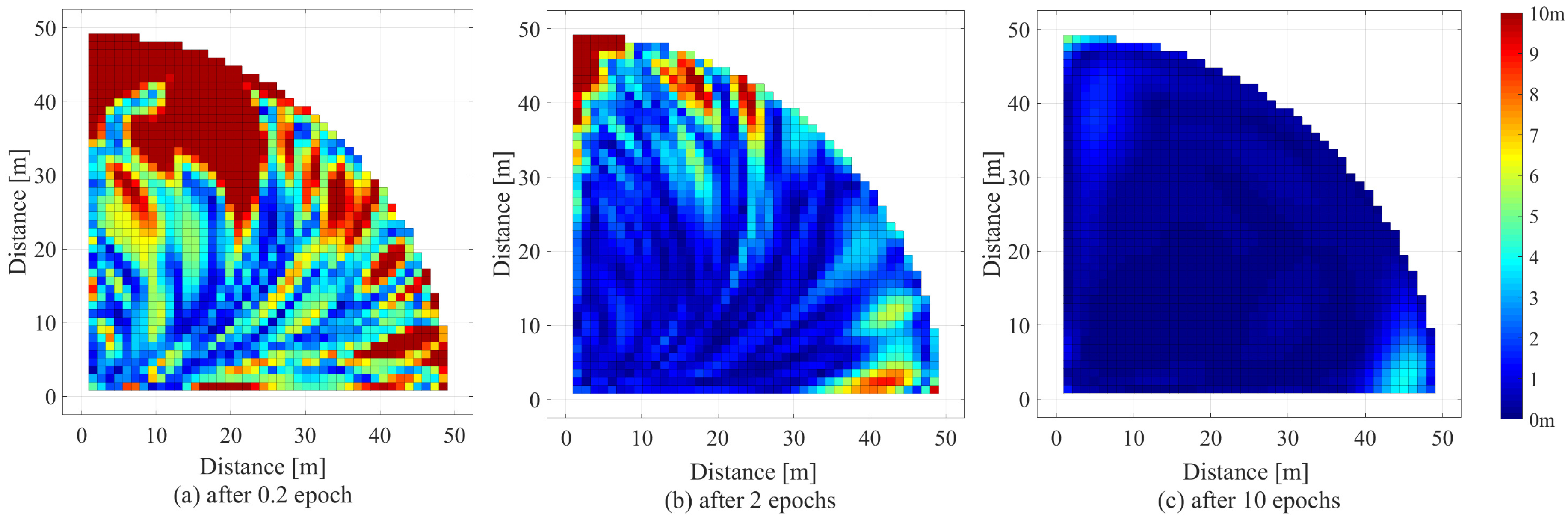
Generating datasets were required to train the DNN. We considered vehicular networks as a circular shaped area with a radius of 50 m in two dimensional space. As our DNN aims to obtain the relative location given two prior locations and relative measurements between them, a quadrants circular sector shaped area with a center at ${[0,0]}^{\mathrm{T}}$ (shown in Figure 3) was utilized in generating datasets for preventing duplicated data training. We defined a dataset between vehicle i at the center and j as ${\mathcal{D}}_{i,j}=\{{\mathbf{x}}_i,{\mathbf{x}}_j,z_{d_{i\to j}},z_{{\theta }_{i\to j}}\}$. The points at which a neighbor vehicle was relatively located with respect to the central vehicle at ${[0,0]}^{\mathrm{T}}$, is ${[dcos\theta ,dsin\theta ]}^{\mathrm{T}}$, where $d\in \{1\mathrm{m},2\mathrm{m},\dots ,50\mathrm{m}\}$ and $\theta \in \{0^{°},1^{°},\dots ,{90}^{°}\}$. To generate the relative measurements, we have added the additive white Gaussian noise to each distance and angle. Specifically, we assume that the error of the distance measurement becomes larger as the distance between vehicles increases. It is based on the fact that the SNR increases as the distance between vehicles becomes shorter to yield better time delay estimation. Therefore, the noisy distance in the dataset is given arbitrarily as $d+d{N}_d/50$ where $N_d$ is a zero mean Gaussian variable with the variance ${\sigma }_d^2$. The standard deviation of the measurement noise ${\sigma }_d$ and ${\sigma }_{\theta }$ are respectively set to 1 m and 1${}^{°}$, and the prior location variance set to 100 ${\mathrm{m}}^2$.

The mean squared error (MSE) method was used to measure the training loss, and we chose Adam as the optimizer. All parameters for DNN architecture were selected to decrease the training loss. Other optimized hyperparameters for the proposed DNN are summarized in Table 1. One epoch indicates the number of datasets for training, and was set to 4550. The data training was performed via Tensorflow.

4.2. Performance Evaluation of Trained DNN

In this section, we show that the proposed DNN technique was successfully applied to the nonlinear function for the measurement update. For evaluating the trained DNN performance as discussed in Section 4.1, the 1000 location samples were randomly generated in the circular area with a radius of 50 m. Considering fact that our dataset has the distance increment of 1 m and the angle increment of $1^{°}$, thus the trained DNN is tested. To test the trained DNN, the errors of the output layer were analyzed when the measurements at two points, randomly chosen in the test region, were imported in the input layer. The test region is the quadrants circular sector area introduced in Section 4.1. Figure 3 shows the analyzed error in the trained DNN. It is clearly shown that the location errors were significantly reduced as the number of epochs increased. The center areas of the test region were trained faster than the edge area. Hence, the edge area had a relative difficulty in learning.

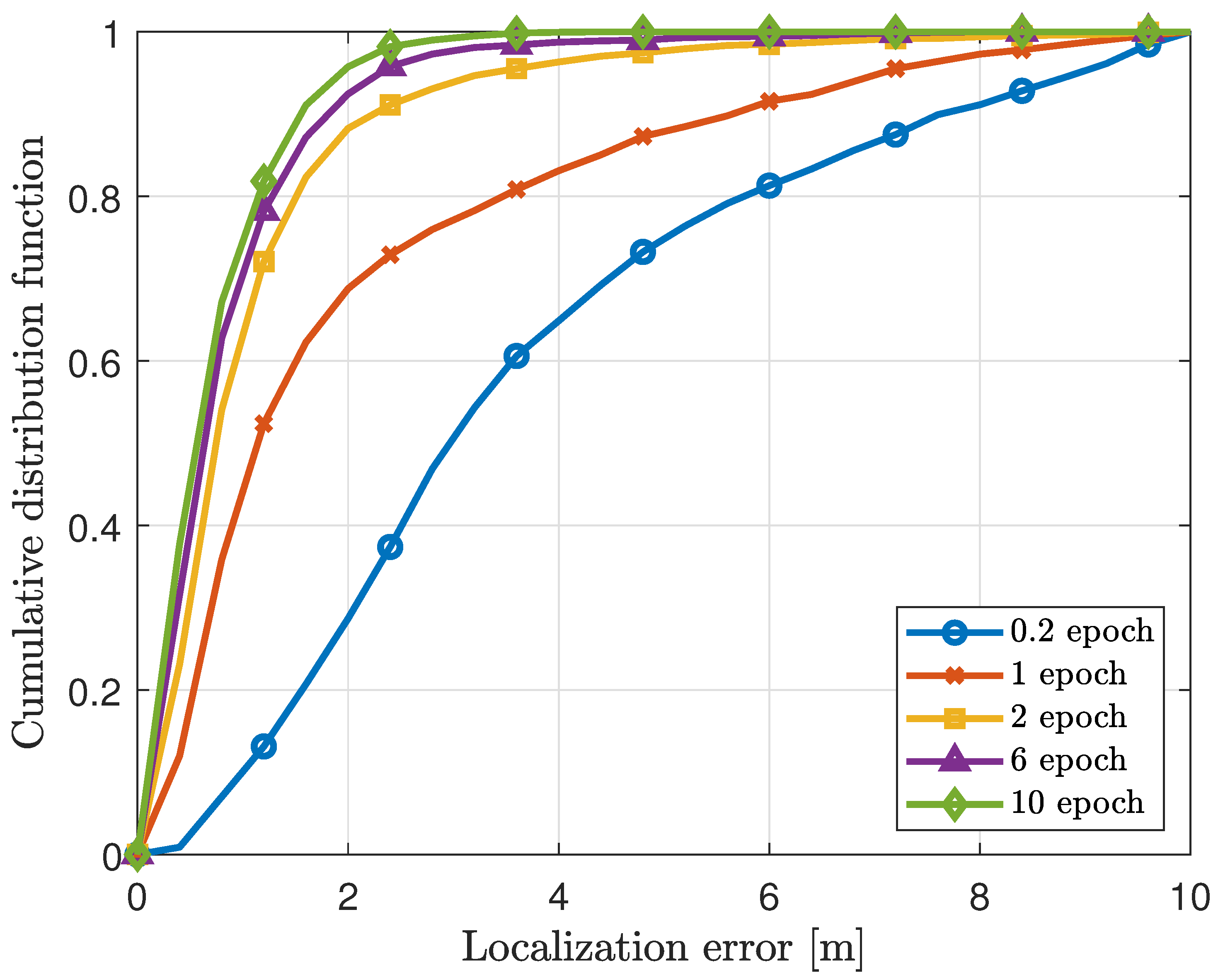
Figure 4 shows the cumulative distribution function (CDF) of the location error with respect to the different number of epoch. The location error for evaluating the trained DNN was measured by the distance between the true location and the output location of the trained DNN. It is clearly shown that the location errors were significantly reduced as the number of epoch increases. As the number of the epoch increased, the DNN became closer to the learning model. For one epoch training, the CDF of the localization error within 1 m was about 0.5. After 10 epochs training, the CDF of the localization error within 1 m was over 0.8. From this result, it is clearly shown that our DNN was reasonably trained.

4.3. Performance of DNN-Assisted Cooperative Localization

We compared our proposed scheme with SPAWN [5] and multilateration (MULT). SPAWN [5] is a cooperative localization algorithm with an Bayesian approach. In SPAWN, to estimate the location of the node, the posterior distribution (3) is calculated, and the belief for implementation is performed by the particle filter. The location estimates by MULT is calculated as

$${\widehat{\mathbf{x}}}_i=\frac{1}{N_i}\sum _{j\in N_i}[z_{d_{i\to j}}cos\left(z_{{\theta }_{i\to j}}\right),z_{d_{i\to j}}sin\left(z_{{\theta }_{i\to j}}\right){]}^{\mathrm{T}}.$$

(8)

Figure 5 shows the CDF of the localization error for demonstrating the effectiveness of DNN-assisted cooperative localization compared to SPAWN and MULT. The number of vehicles I and iterations L were respectively set to 4 and 10. The performance was averaged by 1000 Monte Carlo runs. In SPAWN, the number of used particles was set to 100 for each vehicle, and we chose kernel density estimation for implementing the belief. We analyzed the amount of multiplication of the proposed scheme with SPAWN as shown in

Table 2. Computational complexity of DNN-assisted cooperative localization compared to SPAWN.

Number of Vehicles I	4	5	6	7	8	9
DNN	1.306 × ${10}^5$	2.176 × ${10}^5$	3.264 × ${10}^5$	4.570 × ${10}^5$	6.093 × ${10}^5$	7.834 × ${10}^5$
SPAWN	7.505 $\times 10$ ${}^{10}$	1.251 $\times 10$ ${}^{11}$	1.877 × ${10}^{11}$	2.628 × ${10}^{11}$	3.505 × ${10}^{11}$	4.507 × ${10}^{11}$

. The computational complexity was analyzed by the number of operations. The complexity of SPAWN $C_{\mathrm{SPAWN}}$ was determined as $(IG+G^2)\left(\genfrac{}{}{0pt}{}{I}{2}\right)PL$, where G is the number of grid points and P is the number of particles of each node. The $\left(\genfrac{}{}{0pt}{}{I}{2}\right)$ is defined as the a pair-combination of I vehicles. For the proposed algorithm, the complexity $C_{\mathrm{proposed}}$ is represented as $(L_{\mathrm{in}}{H}_1+H_1{H}_2+H_2{H}_3+H_3{L}_{\mathrm{out}})\left(\genfrac{}{}{0pt}{}{I}{2}\right)L$, where $L_{\mathrm{in}}$ and $L_{\mathrm{out}}$ are the number of nodes at both input and output layers, respectively. $H_k$ is the number of nodes at k-th hidden layer. The location of vehicles was not a determined value in the network, therefore the x-axis of the Figure 5 is considered to be a relative localization error. The average localization error for the proposed model was 0.8937 m, MULT is 1.4289 m, and SPAWN was 0.8926 m. It is clearly shown that our proposed DNN-assisted cooperative localization has significant gain in the computational complexity while sustaining the localization accuracy.

5. Conclusions

In this paper, we propose DNN-assisted cooperative localization in vehicular networks. We elaborate the cooperation procedure to the incorporate DNN in the proposed cooperative localization scheme. By using DNN, we were able to solve a chronic nonlinear approximation problem, and enhance the computational complexity. The greatest advantage of the proposed scheme with DNN is that the cooperative localization becomes much simpler and faster after proper learning with a minimal performance degradation. We expect the proposed scheme will be able to assist the autonomous or self driving vehicles in the future IoV environment.

References

- Closas, P.; Fernandez-Prades, C.; Fernandez-Rubio, J.A. Maximum Likelihood Estimation of Position in GNSS. IEEE Signal Process. Lett. 2007, 14, 359–362. [Google Scholar] [CrossRef] [Green Version]
- Patwari, N.; Ash, J.N.; Kyperountas, S.; Hero, A.O.; Moses, R.L.; Correal, N.S. Locating the nodes: Cooperative localization in wireless sensor networks. IEEE Signal Process. Mag. 2005, 22, 54–69. [Google Scholar] [CrossRef]
- Gustafsson, F.; Gunnarsson, F. Mobile positioning using wireless networks: Possibilities and fundamental limitations based on available wireless network measurements. IEEE Signal Process. Mag. 2005, 22, 41–53. [Google Scholar] [CrossRef]
- Kim, S.; Brown, A.P.; Pals, T.; Itlis, R.A.; Lee, H. Geolocation in ad hoc networks using DS-CDMA and generalized successive interference cancellation. IEEE J. Sel. Areas Commun. 2005, 23, 984–998. [Google Scholar] [CrossRef]
- Wymeersch, H.; Lien, J.; Win, M.Z. Cooperative localization in wireless networks. IEEE Proc. 2009, 97, 427–450. [Google Scholar] [CrossRef]
- Loeliger, H.A. An introduction to factor graphs. IEEE Signal Process. Mag. 2004, 21, 427–450. [Google Scholar] [CrossRef]
- Kschischang, F.R.; Frey, B.J.; Loeliger, H.A. Factor graphs and the sum-product algorithm. IEEE Trans. Inf. Theory 2001, 47, 498–519. [Google Scholar] [CrossRef]
- Baron, D.; Sarvotham, S.; Baraniuk, R.G. Bayesian Compressive Sensing Via Belief Propagation. IEEE Trans. Signal Process. 2010, 58, 269–280. [Google Scholar] [CrossRef]
- Cakmak, B.; Urup, D.N.; Meyer, F.; Pedersen, T.; Fleury, B.H.; Hlawatsch, F. Cooperative localization for mobile networks: A distributed belief propagation–mean field message passing algorithm. IEEE Signal Process. Lett. 2016, 23, 828–832. [Google Scholar] [CrossRef]
- Meyer, F.; Hlinka, O.; Hlawatsch, F. Sigma Point Belief Propagation. IEEE Signal Process. Lett. 2014, 21, 145–149. [Google Scholar] [CrossRef]
- García-Fernández, Á.F.; Svensson, L.; Särkkä, S. Cooperative Localization Using Posterior Linearization Belief Propagation. IEEE Trans. Veh. Technol. 2018, 67, 832–836. [Google Scholar] [CrossRef]
- Kim, S.; Lee, S.H.; Kim, S. Cooperative localization with distributed ADMM over 5G-based VANETs. IEEE WCNC 2018. [Google Scholar] [CrossRef]
- Kim, H.; Choi, S.W.; Kim, S. Connectivity Information-aided Belief Propagation for Cooperative Localization. IEEE Wirel. Commun. Lett. 2018, 7, 1010–1013. [Google Scholar] [CrossRef]
- Mnih, V.; Kavukcuoglu, K.; Silver, D.; Rusu, A.A.; Veness, J.; Bellemare, M.G.; Graves, A.; Riedmiller, M.; Fidjeland, A.K.; Ostrovski, G.; et al. Human-level control through deep reinforcement learning. Nature 2015, 518, 529–533. [Google Scholar] [CrossRef] [PubMed]
- Yu, H.; Tan, Z.H.; Zhang, Y.; Ma, Z.; Guo, J. DNN Filter Bank Cepstral Coefficients for Spoofing Detection. IEEE Access 2017, 5, 4779–4787. [Google Scholar] [CrossRef]
- Jiang, C.; Zhang, H.; Ren, Y.; Han, Z.; Chen, K.; Hanzo, L. Machine Learning Paradigms for Next-Generation Wireless Networks. IEEE Wirel. Commun. 2017, 24, 98–105. [Google Scholar] [CrossRef]
- Ye, H.; Liang, L.; Li, G.Y.; Kim, J.; Lu, L.; Wu, M. Machine Learning for Vehicular Networks: Recent Advances and Application Examples. IEEE Veh. Technol. Mag. 2018, 13, 94–101. [Google Scholar] [CrossRef]
- Li, J.; Mei, X.; Prokhorov, D.; Tao, D. Deep Neural Network for Structural Prediction and Lane Detection in Traffic Scene. IEEE Trans. Neural Netw. Learn. Syst. 2017, 28, 690–703. [Google Scholar] [CrossRef] [PubMed]
- Win, M.Z.; Conti, A.; Mazuelas, S.; Shen, Y.; Gifford, W.M.; Dardari, D.; Chiani, M. Network localization and navigation via cooperation. IEEE Commun. Mag. 2011, 49, 56–62. [Google Scholar] [CrossRef]
- Sze, V.; Chen, Y.H.; Yang, T.J.; Emer, J.S. Efficient Processing of Deep Neural Networks: A Tutorial and Survey. Proc. IEEE 2017, 105, 2295–2329. [Google Scholar] [CrossRef] [Green Version]
- Ferreira, A.G.; Fernandes, D.; Catarino, A.P.; Monteiro, J.L. Performance Analysis of ToA-Based Positioning Algorithms for Static and Dynamic Targets with Low Ranging Measurements. Sensors 2017, 17, 1915. [Google Scholar] [CrossRef] [PubMed]
- Akail, N.; Moralesl, L.Y.; Murase, H. Reliability Estimation of Vehicle Localization Result. In Proceedings of the 2018 IEEE Intelligent Vehicles Symposium (IV), Changshu, China, 26–30 June 2018; pp. 740–747. [Google Scholar]
- Zhang, W.; Liu, K.; Zhang, W.; Zhang, Y.; Gu, J. Deep Neural Networks for wireless localization in indoor and outdoor environments. Neurocomputing 2016, 194, 279–287. [Google Scholar] [CrossRef]
- Adege, A.B.; Yen, L.; Lin, H.P.; Yayeh, Y.; Li, Y.R.; Jeng, S.S.; Berie, G. Applying Deep Neural Network (DNN) for large-scale indoor localization using feed-forward neural network (FFNN) algorithm. In Proceedings of the 2018 IEEE International Conference on Applied System Invention (ICASI), Chiba, Japan, 13–17 April 2018; pp. 814–817. [Google Scholar]
- Nguyen, T.; Jeong, Y.; Shin, H.; Win, M.Z. Machine Learning for Wideband Localization. IEEE J. Sel. Areas Commun. 2015, 33, 1357–1380. [Google Scholar] [CrossRef]
- Ihler, A.T.; Fisher, T.; Moses, R.L.; Willsky, A.S. Nonparametric belief propagation for self-localization of sensor networks. IEEE J. Sel. Areas Commun. 2005, 23, 809–819. [Google Scholar] [CrossRef]
- Dai, W.; Shen, Y.; Win, M.Z. Energy-Efficient Network Navigation Algorithms. IEEE J. Sel. Areas Commun. 2015, 33, 1418–1430. [Google Scholar] [CrossRef]
- Goodfellow, I.; Bengio, Y.; Courville, A. Deep Learning; MIT Press: Cambridge, MA, USA, 2016. [Google Scholar]
- Schmidhuber, J. Deep learning in neural networks: An overview. Neural Netw. 2015, 61, 85–117. [Google Scholar] [CrossRef] [PubMed] [Green Version]
- Kingma, D.P.; Ba, J. Adam: A Method for Stochastic Optimization. arXiv 2014, arXiv:1412.6980. [Google Scholar]
- Srivastava, N.; Hinton, G.; Krizhevsky, I.; Salakhutdinov, R. Dropout: A Simple Way to Prevent Neural Networks from Overfitting. J. Mach. Learn. Res. 2014, 15, 1929–1958. [Google Scholar]
Figure 1.
Vehicular network for cooperative localization. Vehicle 2 observes distance and angle measurement from connected vehicles.
Figure 2.
Deep neural network (DNN)-assisted cooperative and distributed localization algorithm scheme.
Figure 3.
Location error representation of the trained DNN with respect to epochs.
Figure 4.
Localization accuracy of the proposed DNN technique.
Figure 5.
Localization accuracy of the DNN-assisted cooperative localization scheme.