Axial Thrust, Disk Frictional Losses, and Heat Transfer in a Gas Turbine Disk Cavity

Abstract

The gas turbine is a kind of high-power and high-performance energy machine. Currently, it is a hot issue to improve the efficiency of the gas turbines by reducing the amount of secondary air used in the disk cavity. The precondition is to understand the effects of the through-flow rate on the axial thrust, the disk frictional losses, and the characteristics of heat transfer under various experimental conditions. In this paper, experiments are conducted to analyze the characteristics of flow and heat transfer. To ensure the safe operation of the gas turbine, the pressure distribution and the axial thrust are measured for various experimental conditions. The axial thrust coefficient is found to decrease as the rotational speed and the through-flow rate increases. By torque measurements, the amounts of the moment coefficient drop as the rotational speed increases while increase with through-flow rate. In order to better analyze the temperature field within the cavity, both the local and the average Nusselt number are investigated with the help of thermochromic liquid crystal technique. Four correlations for the local Nusselt number are determined according to the amounts of a through-flow coefficient. The results in this study can help the designers to better design the secondary air system in a gas turbine.

1. Introduction

Gas turbines are widely used in the fields of aircraft propulsion and power generation. They play a significant role in the civil economy and national defense. The disk cavity, shown in Figure 1, is a complicated structure of the secondary air system in a gas turbine. It is the wheel space between the rotating disk and the stationary casing. In the disk cavity, the rotating disk is routinely used over a long time to distribute the cold air and prevent the ingress of the hot gas into the cavity through the rim seal. According to the experience of the authors’ group, the amount of secondary air used in the disk cavity comprises around 6% of the mass flow at the compressor inlet [1]. Since it is quite difficult to further improve the efficiency of the compressor stages, it is a promising way to increase the efficiency of a gas turbine by reducing the amount of cooling and sealing air. It requires insight into the pressure distribution, the axial thrust, the disk frictional losses, and the temperature field at each working condition. The foundation and the premise are to investigate the flow and the heat transfer within the basic rotor-stator cavity model (see Figure 1). The flow is firstly extracted from the compressor stages and pumped into the disk cavity. Then it moves radially outwards and cools down both the disk and the wall. Finally, it enters the turbine cascade and prevents the hot gas from entering the cavity. In this study, the receiver holes in the turbine disk are not discussed.

Figure 1. The sketch of the disk cavity in a gas turbine. $z$: axial coordinate (m), $r$: radial coordinate (m), $s$: axial gap width of the front chamber (m), $b$: effective outer radius of the disk (m).

In a rotor-stator cavity, the radial distributions of pressure $p$ are extensively investigated and reported by a lot of researchers. Taking the pressure at the radial position $x=1$ (non-dimensional radial coordinate $x=\frac{r}{b}$) as the reference pressure, the pressure coefficient $C_p$ then is defined in Equation (1) [2,3,4]. As understood, the pressure distributions are primarily influenced by the geometry of the side chamber, the speed of rotation $n$ and $C_w$ [5].

$$C_p=p^{*}\left(x=1\right)-p^{*}\left(x\right) ; p^{*}=\frac{p}{\rho ·{\Omega }^2·b^2}$$

(1)

where $p^{*}$ is the non-dimensional pressure, $\rho$ is the density of the fluid ($\mathrm{kg}/{\mathrm{m}}^3$), $\Omega$ is the angular velocity of the disk ($\mathrm{rad}/\mathrm{s}$).

The well-known correlation which associates the pressure with the core swirl ratio $K$ is written in Equation (3) [4,5].

$$\frac{\partial p}{\partial r}=\rho ·K^2·{\Omega }^2·r$$

(2)

where $K$ is the core swirl ratio.

The parameter $K$, defined in Equation (3), is the ratio of the angular velocity of the fluid at half of the axial gap width $\zeta =0.5$ to that of the disk.

$$K=\frac{{\Omega }_f}{\Omega } at \zeta =0.5 ; \zeta =\frac{z}{s}$$

(3)

where ${\Omega }_f$ is the angular velocity of the fluid, $\zeta$ is the non-dimensional axial coordinate.

In the disk cavity, there are three flow types (Stewartson type, Batchelor type, and Couette type), based on which the amounts of $K$ are calculated. Owen and Rogers [4] distinguished the Batchelor type flow based on the turbulent flow parameter ${\lambda }_t$, defined in Equation (4). The parameter ${\lambda }_t$ weighs the relative strength of the viscous and the inertial force of the through-flow.

$${\lambda }_t=\frac{C_w}{R{e}^{0.8}} ; C_w=\frac{\dot{m}}{\mu ·b} ; Re=\frac{\Omega ·b^2}{\nu }$$

(4)

where ${\lambda }_t$ is the turbulent flow parameter, $C_w$ is the through-flow coefficient, $Re$ is the global circumferential Reynolds number, $\dot{m}$ is the mass flow rate ($\mathrm{kg}/\mathrm{s}$), $\mu$ is the dynamic viscosity ($\mathrm{N}·\mathrm{s}/{\mathrm{m}}^2$), $\nu$ is the kinematic viscosity (${\mathrm{m}}^2/\mathrm{s}$).

Poncet et al. [5,6] distinguished between the Stewartson type flow and the Batchelor type flow according to the values of the local flow rate coefficient $C_{qr}$, written in Equation (5). Will et al. [7,8] associated the radial pressure distributions with both the tangential and the radial velocities for either Batchelor type or Couette type flow. By numerical simulations, Hu et al. [9,10] determined part of the boundaries between the Batchelor type flow and the Couette type flow in a rotor-stator cavity with through-flow. Debuchy et al. [11] investigated the flow behavior of the Batchelor type flow. They stated that the flow in the rotor boundary layer was assumed to behave as expressed by Owen and Rogers [4] in the case of a turbulent flow on a rotating single disk. On the stator side, a necessary compensation flow rate must take place according to the conservation of mass. It was found that this compensation flow rate could not be estimated with a good accuracy using the hypotheses of a stationary disc in a rotating fluid in [4].

$$C_{qr}=\frac{Q_t·R{e}_{\phi }{}^{0.2}}{2·\pi ·\Omega ·r^3} ; R{e}_{\phi }=\frac{\Omega ·r^2}{v}$$

(5)

where $Q_t$ is the volumetric flow rate (${\mathrm{m}}^3/\mathrm{s}$), $R{e}_{\phi }$ is the local circumferential Reynolds number.

The demands for the safe operation and long service life require the precise prediction on the axial thrust. By force measurements, Bo Hu et al. [9,10] determined some empirical correlations of the axial thrust coefficient $C_F$, defined in Equation (6), in the side chambers of centrifugal pumps. Kurokawa et al. [12,13] studied the variations of $C_F$ in the casing of a radial flow turbomachine with leakage flow. They stated that there was a positive correlation between $C_F$ and the angular momentum at the inlet. The values of $C_F$ showed little change when the inlet angular momentum of the leakage flow is a constant. The disadvantage of the correlations is that they are only valid for $G=$ {0.018, 0.036, 0.054, 0.072} in [9,10] and $G=$ {0.024, 0.048, 0.097} in [12,13]. The parameter $G$ is the non-dimensional axial gap width, defined in Equation (7). Currently, the results of $C_F$ are far from enough to be used to determine a more extensive empirical correlation.

$$C_F={\int }_0^b\frac{2·\pi ·\left(p_b-p\right)·r\mathrm{d}r}{\rho ·{\Omega }^2·b^4}$$

(6)

where $p_b$ is the pressure at the outer radius of the disk (Pa), $p$ is the pressure (Pa).

$$G=\frac{s}{b}$$

(7)

In a rotor-stator cavity, reducing the amounts of the disk frictional losses is always one of the hot focuses in the researches, which are aimed to improve the efficiency. The moment coefficient $C_M$ is defined in Equation (8). Owen et al. [4] found the relationship between $C_M$ and ${\lambda }_t$. Hu et al. [9,10] extended part of the Daily&Nece Diagram into three dimensions with a third axis of $C_w$. They also organized two empirical correlations of $C_M$ for the two turbulent flow regimes (turbulent flow with either small or large axial gap width). Kurokawa et al. [12,13] experimentally investigated the disk frictional losses and found that the disk frictional torque showed little change with a fixed inlet angular momentum. Wang et al. [14] conducted a combined energy loss model to lower the disk frictional losses in the side cavity of a centrifugal pump. They found that the interstage leakage loss was converted by the disk frictional loss, while the volumetric leakage loss was negatively correlated with the disk frictional loss.

$$C_M=\frac{2·\left|M\right|}{\rho ·{\Omega }^2·b^5}$$

(8)

where $M$ is the frictional torque on a single surface ($\mathrm{Nm}$).

The investigations on the characteristics of heat transfer is one of the key factors to precisely predict the temperature field within the cavity and the fatigue strength of the components. A lot of studies were conducted introducing the experimental technique and numerical simulations in the past. With remote infrared sensors, Metzger et al. [15] measured the radial distributions of the local heat transfer coefficient $h$, defined in Equation (9). According to their results, the heat transfer can be enhanced when the parameters, such as $Re$, $C_w$, and $G$, are synthetically optimized. Metzger et al. [16] determined a correlation, which enabled to estimate the amounts of $h$ with the help of the transient TLC (thermochromic liquid crystal) technique. Taler et al. [17,18] conducted a detailed derivation of the correlation. Taler et al. [18] also discussed other transient inverse methods for determining the amounts of $q$ (heat flux) and $h$. Metzger’s research group [16,19,20] and Luo et al. [21] used the transient TLC technique to measure the radial distributions of $h$. Poncet et al. [22] performed the numerical investigations of the flow and the heat transfer inside a rotor-stator cavity. The results from the established Reynolds stress model agreed well with the experimental results.

$$h=\frac{-q}{\left(T_{aw}-T_w\right)} ; T_{aw}=T_{\infty }+r_{rec}·\frac{u_{\infty }{}^2}{2·l} ; r_{rec}\approx P{r}^{0.5} ; Pr=\frac{\mu ·l}{k}$$

(9)

where $q$ is the heat flux ($\mathrm{W}/{\mathrm{m}}^2$), $T_{aw}$ is the adiabatic wall temperature (K), $T_w$ is the surface temperature (K), $T_{\infty }$ is the temperature of the mainstream at $\zeta =0.5$ (K), $r_{rec}$ is the recovery factor, $u_{\infty }$ is the velocity of the mainstream at $\zeta =0.5$ ($\mathrm{m}/\mathrm{s}$), $l$ is the specific heat at constant pressure ($\mathrm{J}/\left(\mathrm{kg}·\mathrm{K}\right)$, $Pr$ is the Prandtl number, $k$ is the thermal conductivity ($\mathrm{W}/\left(\mathrm{m}·\mathrm{K}\right)$).

The average convective heat transfer coefficient $h_{ave}$ on the disk surface is computed as

$$h_{ave}=\frac{{\int }_{r_c}^{b}2hrdr}{b^2-r_c{}^2}$$

(10)

where $r_c$ is the inner radius where the measurements of $h$ start.

The heat transfer coefficient can be transformed to the non-dimensional form, namely the Nusselt number. The local Nusselt number $N{u}_r$ and the average Nusselt number $N{u}_{ave}$ are defined in Equation (11). Tuliszka-Sznitko et al. [23] and Majchrowski et al. [24] performed the large-eddy simulation for the distributions of $N{u}_r$, along both the stator and the rotor. Liao et al. [25] determined a series of correlations of $N{u}_r$. They put forward that $\ln (N{u}_r)$ was approximately linear with the increase of $\ln (R{e}_{\phi })$. Luo et al. [21] found that the amounts of $N{u}_{ave}$ should be predicted according to the flow sections in the disk cavity. Lin [1] stated that both the flow in the boundary layer and the heat conductivity in the disk should be considered to estimate the values of $N{u}_{ave}$.

$$N{u}_r=\frac{h·r}{k} ; N{u}_{ave}=\frac{b·{\int }_{r_c}^b\frac{2hrdr}{k}}{\left(b^2-r_c{}^2\right)}$$

(11)

Although a lot of studies have been conducted, both the flow and the heat transfer are not discussed synthetically in the disk cavity. In addition, when the rotational speed of the shaft changes, the effects of the through-flow rate on the above parameters are still insufficiently studied. To reduce the amount of secondary air, which is extracted from the compressor, this paper is aimed to provide some results on how the parameters such as $C_p$, $C_F$, $C_M$, $N{u}_r$, and $N{u}_{ave}$ change at different experimental conditions. The obtained results can help the designers to reduce the amount of air used in the disk cavity reasonably.

2. Experimental Set-Ups

2.1. Designs of the Test Rigs

The measurements are conducted with two test rigs. The first one, noted as SRSCA, is used to perform the measurements of the pressure, the axial thrust, and the disk frictional losses. A sketch of the longitudinal section of it is depicted in Figure 2a [9,10]. A centrifugal pump system is used to supply the water to the test rig. The speeds of rotation are changed with the help of a frequency converter. The measurements of pressure are performed by means of seven pressure tubes on the stator along the radius. There are three tension-compression sensors to measure the axial thrust. A torque meter is installed between the shaft and the electric motor to measure the torque. A detailed introduction of the test rig SRSCA and the experimental methods are introduced in [9,10]. Unlike previous studies, the value of $G$ is 0.1, which is consistent with the geometry of a gas turbine disk cavity, instead of $0.018, 0.036, 0.054$, and $0.072$ in [9,10]. The geometry of the second test rig for the measurements of $h$, noted as SRSCB, is shown in Figure 2b. The front cover is made of plexiglas. The experimental fluid is air. Before entering the rotor-stator cavity, the air is heated in a mesh heater. The temperature rise of 40 K to 60 K in the disk cavity takes less than 100 s. A transient method using TLC is applied for the measurements of $h$. The target disk is firstly painted black and then sprayed with the SPN100R35C1W type TLC in a fan shape region with an angle of ${60}^{°}$. To calculate the Nusselt number, the thermal conductivity of air is calculated according to the temperature [26] in the mainstream (the parameter $k$ is considered as a fixed value every 1 mm). To measure the temperature of the mainstream ($T_{\infty }$), six K-type thermocouples are installed, which are distributed along the radius at $x=\left\{0.4, 0.52, 0.64, 0.76, 0.86, 0.96\right\}$ [1]. The least-square method is used to fit the measured $T_{\infty }$ into the proper $T_{\infty }-x$ curve under each experimental condition. There is a photoelectric switch to trigger the CCD camera. Since no step change in the mainstream occurs, a series of small step superposition is adopted to approximate the curve of the temperature rise in the mainstream. According to the discoloration time of the TLC, the radial distributions of $h$, therefore, are estimated with Equation (12) [16]. The detailed descriptions of the test rig SRSCB and the measuring method of $h$ are referred to [1]. The main parameters of the test rigs are listed in Table 1.

$$T_w-T_i={\displaystyle \sum _{j=1}^n}[1-e^{\left(\frac{h^2·\alpha ·\left(t-t_j\right)}{k^2}\right)}·erfc\left(\frac{h·\sqrt{\alpha ·\left(t-t_j\right)}}{k}\right)]·\left[\Delta T_{\infty \left(j,j-1\right)}\right]$$

(12)

where $T_i$ is the initial temperature on the disk surface (K), $t$ is the time (s), $\alpha$ is the thermal diffusivity (${\mathrm{m}}^2/\mathrm{s}$).

Figure 2. Sketch maps of the test rigs (not to scale): (a) SRSCA and (b) SRSCB.

Table 1. Main parameters of the test rigs in this study.

	$\mathit{b}$ (m)	${\mathit{r}}_{\mathit{o}}$ (m)	$\mathbf{s}$ (m)	${\mathit{s}}_{\mathit{b}}$ (m)	$\mathbf{\Delta }\mathit{r}$ (m)	${\mathit{s}}_{\mathit{o}}$ (m)	$\mathit{n}$ (m)
SRSCA	0.11	0.05	0.011	0.008	0.002	0.002	500–2500
SRSCB	0.25	0.07	0.025	−	−	0.002	500–2500

2.2. Experimental Conditions

Since the geometries of the two test rigs are different, it is quite important to ensure that the two key parameters, namely ${\lambda }_t$ and $G$, are equal from the two test rigs at each measured experimental condition. The approach we use is to make sure the values of $Re$, $G$, and $C_w$ are equal at each experimental condition. For the test rig SRSCB, the value of $Re$ reaches $1.106\times {10}^6$ at $n=2500 \mathrm{rpm}$. To obtain the same value of $Re$, the speed of rotation of the test rig SRSCA is 800 rpm. The maximum speeds of rotation for SRSCA and SRSCB in this study are therefore $800 \mathrm{rpm}$ and $2500 \mathrm{rpm}$. To obtain the same amounts of $C_w$, the values of $\dot{m}$ under each experimental condition, listed in Table 2, are calculated with Equation (13). The flow rate is adjusted by a throttle valve and measured by a flowmeter in each test rig. The parameter $\varsigma$, defined in Equation (14), is the ratio of the current rotational speed to the maximum speed of rotation of each test rig. The experiments are not conducted under the condition $C_w=0$ with the test rig SRSCB.

$$\dot{m}=\mu ·b·C_w$$

(13)

$$\varsigma =\frac{n}{n_{max}}$$

(14)

where $n_{max}$ is the maximum speed of rotation for each test rig.

Table 2. List of experimental conditions.

$\mathit{\varsigma }$	20%	30%	50%	70%	80%	90%	100%
${\mathit{C}}_{\mathit{w}}$	0	1262	2525	3787	5050

2.3. Uncertainty Analysis

The measured range of the pressure transducer is up to $2.5$ bar (absolute pressure). The measured range of the thrust transducers and the torque meter are $-100 \mathrm{N}~100 \mathrm{N}$ and $0 \mathrm{Nm}~10 \mathrm{Nm}$. The parameter ranges of the output voltage signals are as follows: from $0 \mathrm{V}$ to $10 \mathrm{V}$ for both the pressure transducer and the torque meter, while from $-10 \mathrm{V}$ to $10 \mathrm{V}$ for the axial thrust transducer. The absolute accuracy of the data acquisition system is 4.28 mV. The relative error of the pressure transducer, the torque transducer, and the axial thrust transducer are 1% (FS), 0.1% (FS), and 0.5% (FS), respectively. The uncertainties of the measured results are calculated with the root sum squared method. Each result of $C_p$ (defined in Equation (1)), $C_F$, and $C_M$ is the average value of 1000 samples. The distributions of the results are considered as the normal distributions, whose distribution coefficient is 1.96 (95% confidence level). The uncertainties of the measured pressure, axial thrust, and frictional torque are 40.4 (Pa), 0.024 (N), and 3 $\times {10}^{-4}$ (Nm), which are calculated in [9]. Then the corresponding uncertainties of $C_p$, $C_F$, and $C_M$ are plotted versus $\varsigma$ in Figure 3.

Figure 3. Part of the uncertainties from the measurements.

The accuracies of the measurements of $h$ are greatly influenced by the thickness of the TLC (around 100 $\mathsf{\mu }\mathrm{m}$ in this study), the thermal radiation from the light source and the error of the thermocouples ($\pm$0.2 K). The uncertainties of $h$ are up to 8.3% [1]. The maximum uncertainty of 8.3% is calculated with the equation: $Uncertaint{y}_{max}=\sqrt{7{\%}^2+4.5{\%}^2}$ (7% is the component of the uncertainty due to the sprayed TLC, while 4.5% is the component attributed to the set-ups of the experiments [1]).

3. Results and Discussion

3.1. Radial Pressure Distribution

Figure 4 compares the radial distribution of $C_p$ with different $C_w$ at $\varsigma =20\%$. It is clear that the parameter $C_p$ shows a decreasing trend at each radial coordinate as $C_w$ increases. The parameter $C_p$ increases towards the shaft at fixed $Re$ and $C_w$ values.

Figure 4. Radial distributions of $C_p$ at $\varsigma =20\%$ from measurements.

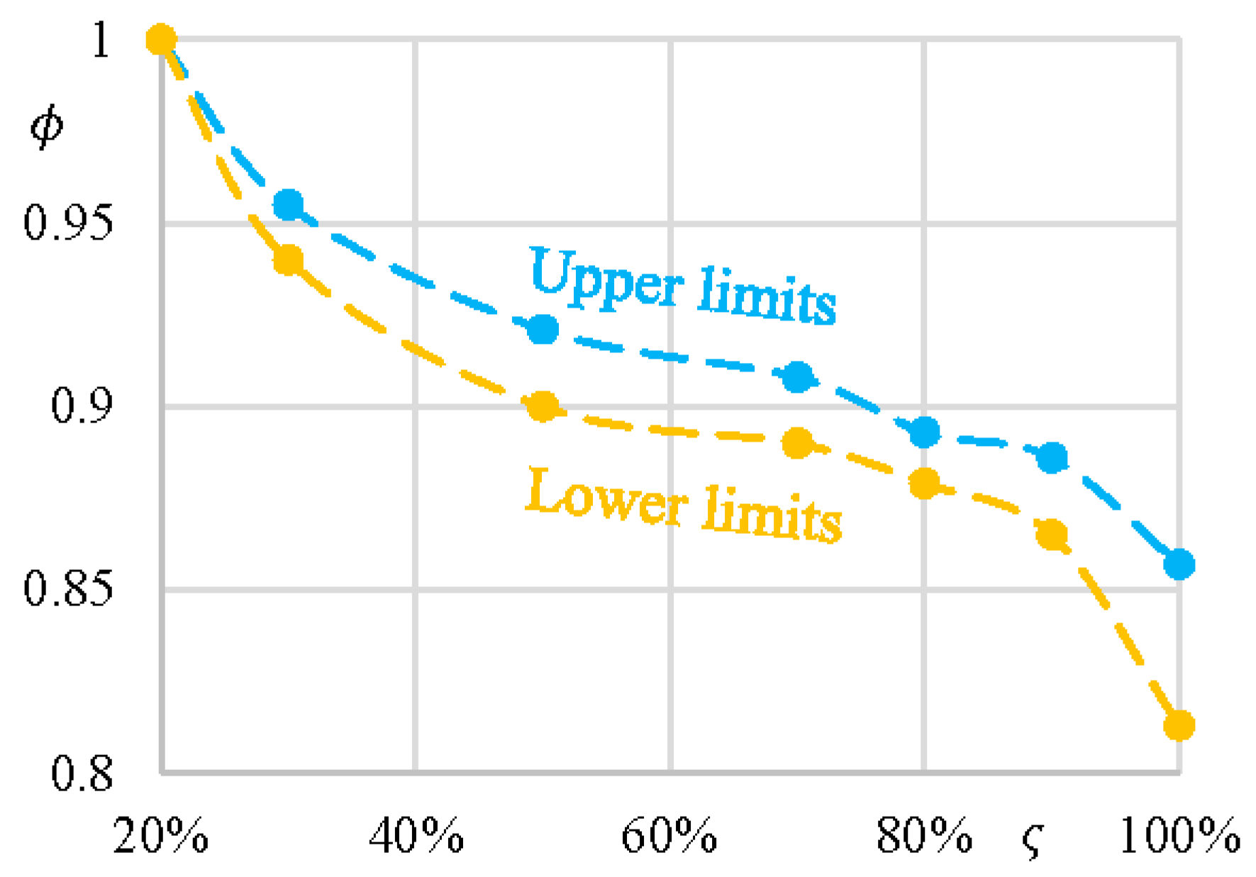
The parameter $\varphi$, defined in Equation (15), is used to show the impacts of $\varsigma$ on $C_p$. The results are shown in Figure 5. The value of $Re$ increases as $\varsigma$ increases. With the increase of $\varsigma$, the amounts of $\varphi$ decrease. The values of $\varphi$ decrease by 15% to 19% when $\varsigma$ arrives at the maximum value. With the increase of $\varsigma$, the maximum and the minimum values of $\varphi$ are compared in Figure 6 for various $C_w$. In the parameter ranges $20\%\le \varsigma \le 30\%$ and $75\%\le \varsigma \le 100\%$, a substantial decrease of $\varphi$ is found. The decrement, however, becomes smaller with the increase of $\varsigma$ in the parameter range: $30\%<\varsigma <75\%$.

Figure 5. Variations of $\varphi$ along the radius from measurements.

Figure 6. General variations of $\varphi$ versus $\varsigma$ from measurements.

$$\varphi =\frac{C_p}{C_p at \varsigma =20\%} at a fixed C_w value$$

(15)

3.2. Axial Thrust Coefficient

The changes in the pressure led to the variations of the axial thrust. On the basis of experimental results, the values of $C_F$ decrease with increasing $C_w$ for $\varsigma =20\%$, shown in Figure 7a. The trend is in accordance with those in [10]. With the decrease of $C_w$, the tangential velocity of the fluid will increase at the position half of the axial gap width [6]. The pressure then will drop significantly towards the shaft, which results in an increase of $C_F$. The parameter $\psi$, written in Equation (16), is used to show the drop ratio of $C_F$. As $\varsigma$ increases, the amounts of $C_F$ drop, shown in Figure 7b. When the values of $\varsigma$ increase from 20% to 30%, the amounts of $C_F$ drop by at least 12.2%. The decrements of $C_F$ become smaller as $\varsigma$ further increases in general. When $\varsigma$ increases from 20% to 100%, the values of $\psi$ plunge to around 60%. The parameter $C_F$ appears to be significantly affected by $\varsigma$.

Figure 7. Axial thrust coefficient from the measurements: (a) Increase of $C_F$ versus $C_w/C_{w,max}$ for $\varsigma =20\%$ and (b) Variations of $\psi$ versus $C_w/C_{w,max}$ for $\varsigma \ge 30\%$.

$$\psi =\frac{C_F}{C_F at \varsigma =20\% } at a fixed C_w value$$

(16)

3.3. Moment Coefficient

To reduce the pollutant emitted into the air, the efficiencies of the gas turbine should be improved. One of the important means is to reduce the disk frictional losses and the leakage losses under different working conditions. The key is to determine how the amount of air impacts the moment coefficient. At the working condition $\varsigma =20\%$, the values of $C_M$ increase with increasing $C_w$, shown in Figure 8a. The increasing trends are in accordance with those in [10]. It is speculated that the gradient of the tangential velocity near the rotor surface increases with the increase of $C_w$, which results in the rise of the wall shear stress [13]. The parameter $\gamma$, defined in Equation (17), is used to show the variations of $C_M$ with increasing $\varsigma$. As shown in Figure 8b, the numbers of $\gamma$ fluctuate with the increase of $C_w$. As $\varsigma$ increases, the amounts of $C_M$ decrease in general, shown in Figure 8b. When $\varsigma$ increases from $20\%$ to $100\%$, the values of $C_M$ drop by around 17.5%.

Figure 8. Moment coefficient from the measurements: (a) Increase of $C_M$ versus $\frac{C_w}{C_{w,max}}$ at $\varsigma =20\%$ and (b) Variations of ${\rm Y}$ versus $\frac{C_w}{C_{w,max}}$ for $\varsigma \ge 30\%$.

$${\rm Y}=\frac{C_M}{C_M at \varsigma =20\% } at a fixed C_w value$$

(17)

3.4. Local Heat Transfer Coefficient

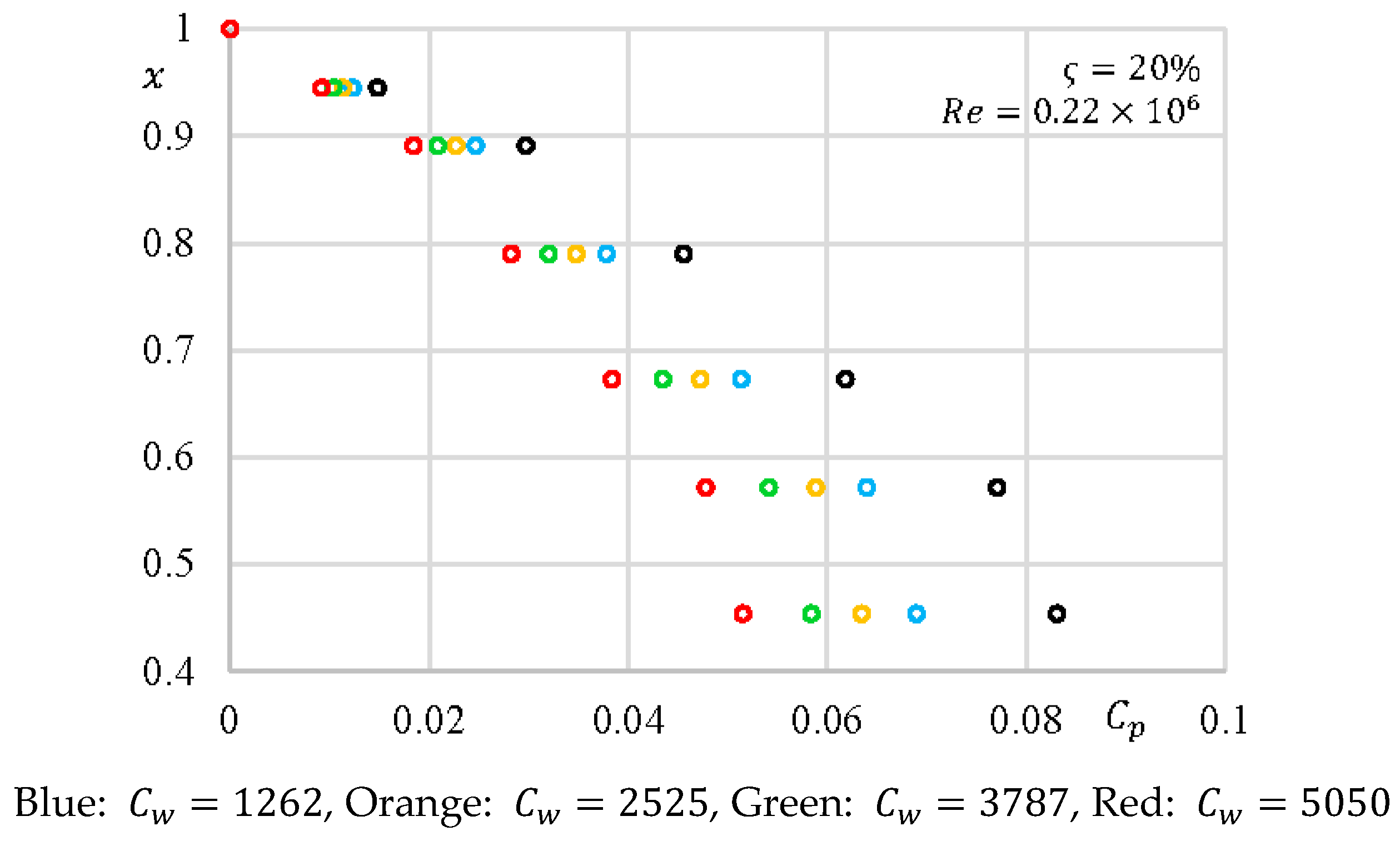
According to the measurements, the radial distributions of $h$ are plotted versus $C_w$ in Figure 9a for $\varsigma =20\%$ ($Re=0.22\times {10}^6$). Four values of $C_w$ are investigated, namely 1262, 2525, 3787, and 5050. Each value of $h$ is the average values at three circumferential positions on the fan-shaped TLC ($0^{°}, {30}^{°}, \mathrm{and} {60}^{°}$) at a certain radial coordinate. The amounts of $h$ decrease toward the outer radius of the disk. At a lower radius, the values of $h$ are relatively larger. The rise of $C_w$ contributes to stronger local heat transfer capacity. As $C_w$ increases, the increments are much larger at a low radius. In the literature such as those in [25], the effects of $C_w$ and $R{e}_{\phi }$ on the distributions of $N{u}_r$ have been discussed. The amounts of $N{u}_r$ are estimated with the power law, written in Equation (18) [25]. Figure 9b illustrates the effects of $R{e}_{\phi }$ on $N{u}_r$. With the increase of $\ln \left(R{e}_{\phi }\right)$, the values of $\ln \left(N{u}_r\right)$ increase in general. The amounts of $\ln \left(N{u}_r\right)$ increase as $C_w$ increases. The increases in $\ln \left(N{u}_r\right)$ versus $\ln \left(R{e}_{\phi }\right)$ become less intense when $C_w$ increases.

Figure 9. Characteristics of heat transfer at $\varsigma =20\%$ ($Re=0.22\times {10}^6$) by measurements: (a) Variations of $h$ along the radius and (b) Variations of $\ln \left(N{u}_r\right)$ versus $\ln \left(R{e}_{\phi }\right)$.

$$N{u}_r=a·R{e}_{\phi }{}^c$$

(18)

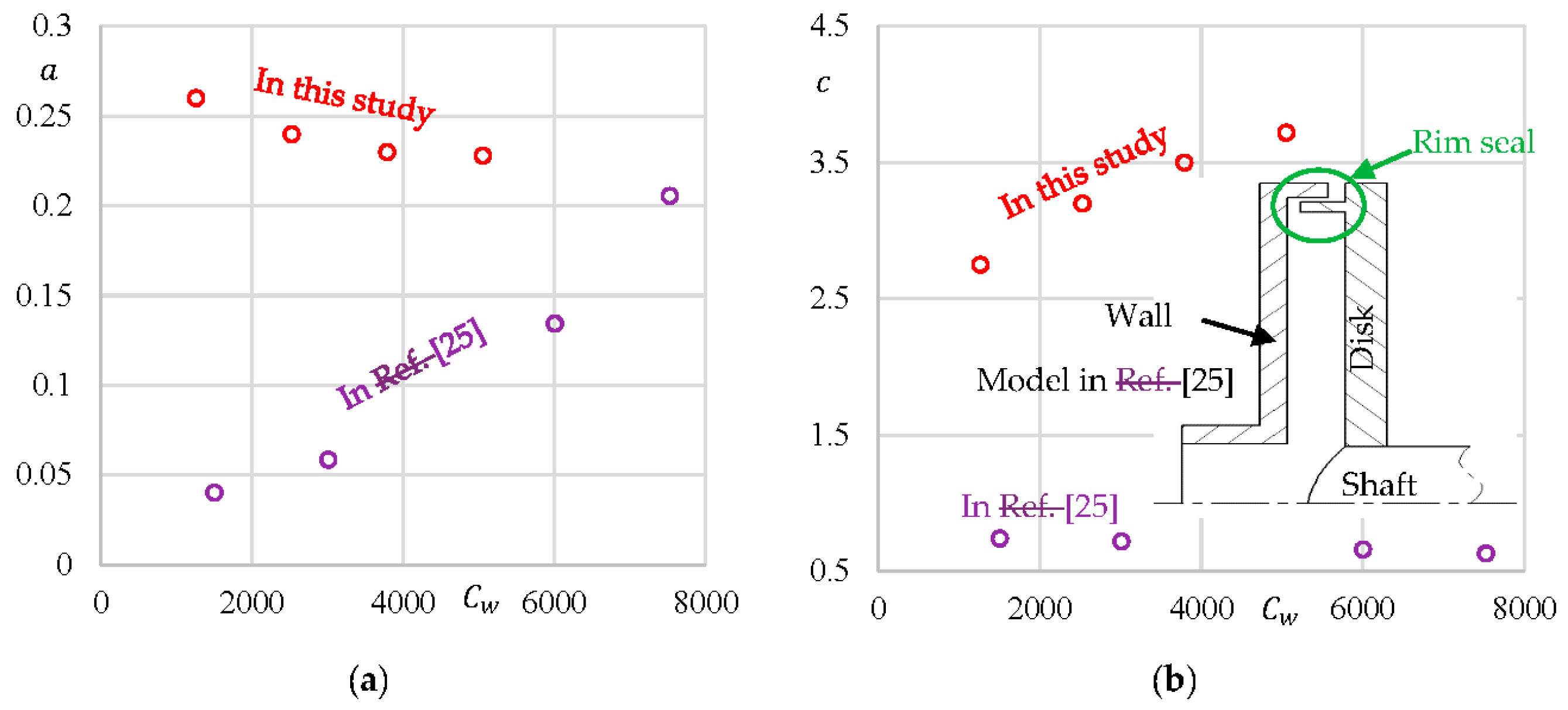
On the basis of the experimental results, the variations of $R{e}_{\phi }$ on $N{u}_r$ for four values of $\varsigma$ (or $Re$) and four values of $C_w$ are depicted in Figure 10. The increases of $\ln \left(N{u}_r\right)$ follow the same trend for the four values of $Re$ at a fixed $C_w$ value in general. The values of the constants in Equation (18) ($a$ and $c$) are determined with the method of least-square. The method simplifies the determinations of the above two parameters. The drawback, however, is that this reduces the accuracy of determining the parameters in Equation (18). It is noted that for $\varsigma =20\%$ and $C_w=5050$, the increment of $\ln \left(N{u}_r\right)$ versus $\ln \left(R{e}_{\phi }\right)$ become smaller in the parameter range: $\ln \left(R{e}_{\phi }\right)\ge 11.7$. Above results also have big disparity with those from the determined correlations. The differences deserve further investigations. The values of $a$ decline as $C_w$ increases while those of $c$ increase with the increase of $C_w$.

Figure 10. Variations of $\ln \left(N{u}_r\right)$ versus $\ln \left(R{e}_{\phi }\right)$ by measurements: (a) $C_w=1262$; (b) $C_w=2525$; (c) $C_w=3787$ and (d) $C_w=5050$.

In Figure 11, the amounts of $a$ and $c$ are compared with those in [25]. The results of $a$ and $c$ by measurements in this paper are much larger than those by numerical simulations in [25]. The variations also show the different trends. The discrepancies cannot be answered from the available data. In [25], there is a rim seal at the outer radius of the cavity, while the cavity is directly connected to the environment in this paper. It is, therefore, speculated that the large differences are due to the difference of the geometry at the outlet of the disk cavity, which obviously results in the different temperature gradients.

Figure 11. Comparison of the constants in Equation (18): (a) Values of $a$ and (b) Amounts of $c$.

3.5. Average Nusselt Number

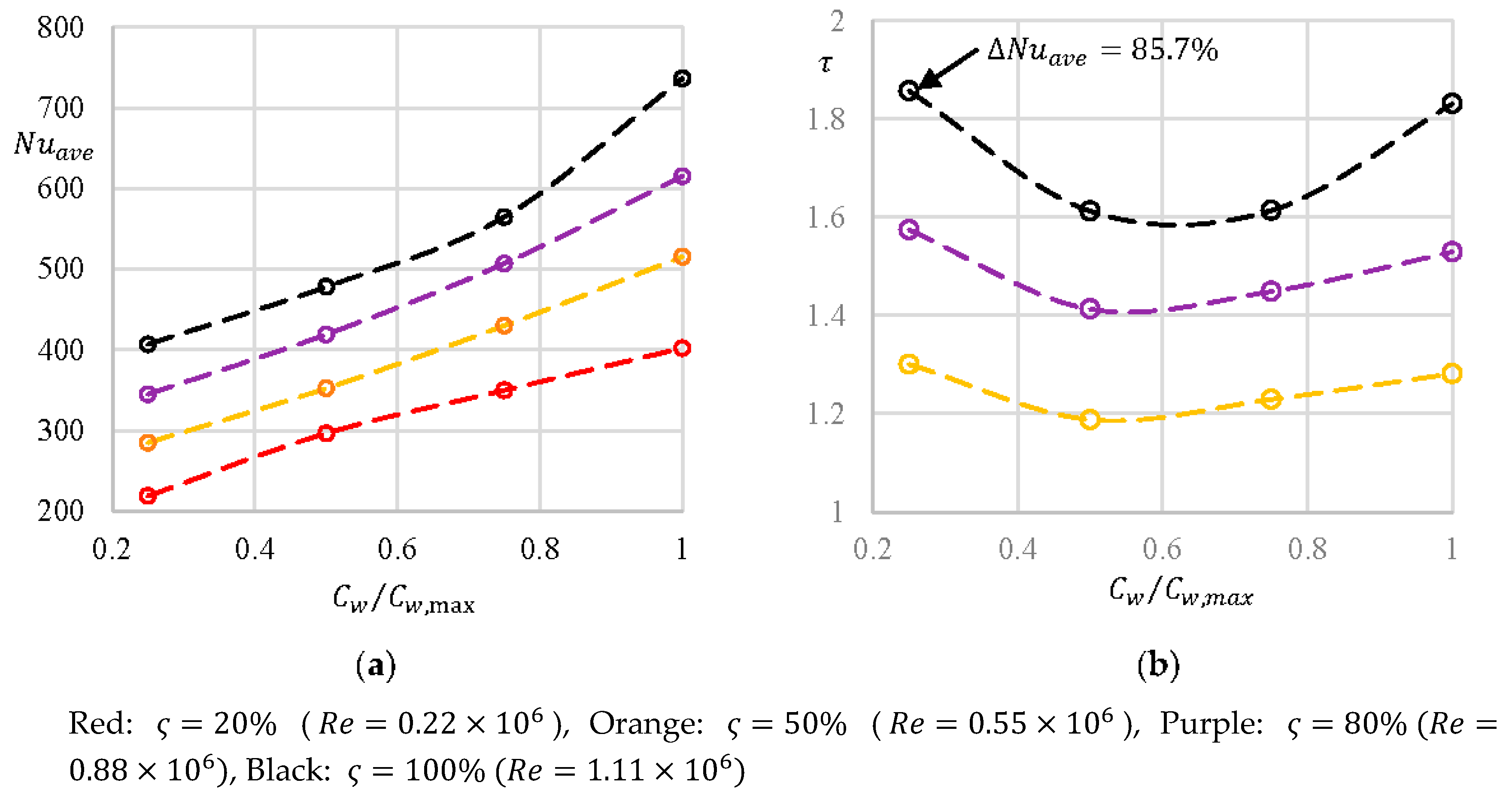
In a rotor-stator cavity, the performances of heat transfer besides the flow patterns are decided by ${\lambda }_t$. The parameter $N{u}_{ave}$ is used to show the average heat transfer capacity. Figure 12a depicts the changes in $N{u}_{ave}$ for various $C_w$. With the increase of $\varsigma$ as well as $Re$, the values of $N{u}_{ave}$ increase. The same trends can also be found in [21]. The parameter $\tau$, written in Equation (19), is used to show the change rate of $N{u}_{ave}$. The parabolic-shaped $\tau -C_w/C_{w,\max }$ curves are depicted in Figure 12b. The amounts of $N{u}_{ave}$ increase by up to 85.7% when $\varsigma$ increases from 20% to 100%. The special shape of $\tau$ deserves further investigations.

Figure 12. Comparison of the heat transfer performances: (a) Changes of $N{u}_{ave}$ versus $C_w/C_{w,\max }$ and (b) Variations of $\tau$ versus $C_w/C_{w,\max }$.

$$\tau =\frac{N{u}_{ave}}{N{u}_{ave} at \varsigma =20\%} at a fixed C_w value$$

(19)

When $\left|{\lambda }_t\right|$ is not large enough, the parameter $\frac{N{u}_{ave}}{R{e}^{0.8}}$ is primarily affected by ${\lambda }_t$ in a rotor-stator system [1,4]. In this study, the values of $\left|{\lambda }_t\right|$ do not exceed 0.3, which is in the parameter range: ${\lambda }_t\le 1.6$ [4,21]. The parameter $\frac{N{u}_{ave}}{R{e}^{0.8}}$ is, therefore, analyzed according to ${\lambda }_t$. It is noted that the exponent value of 0.8 is typical for turbulent boundary layers, as put forward by Schlichting [27]. Aus der Wiesche [28] pointed out that small deviations exist with regard to the exact exponent value in the literature. However, it should be remarked that these deviations are typical of minor importance in comparison with the experimental uncertainty levels occurring in actual systems. The amounts of $\frac{N{u}_{ave}}{R{e}^{0.8}}$ increase with the increase of ${\lambda }_t$, shown in Figure 13. The values of $\frac{N{u}_{ave}}{R{e}^{0.8}}$ are almost in a linear relationship with ${\lambda }_t$ at a fixed $Re$ value.

Figure 13. Variations of $\frac{N{u}_{ave}}{R{e}^{0.8}}$ versus ${\lambda }_t$.

4. Conclusions

In this paper, the characteristics of the flow and the heat transfer in a disk cavity model are investigated by experiments. Some conclusions are as follows:

With the increase of $\varsigma$, the amounts of $C_p$ decrease. Both the upper and the lower limits are found for the drops of $C_p$ with increasing $\varsigma$ at different experimental conditions.

The values of $C_F$ and $C_M$ decrease with increasing $C_w$ or $\varsigma$. With the increase of $\varsigma$, the decrement of $C_F$ is much larger than that of $C_M$ at fixed $Re$ and $C_w$ values.

The values of $h$ increase with increasing $C_w$. Four correlations of $N{u}_r$ and $R{e}_{\phi }$ are summarized according to the amounts of $C_w$. The parameter $N{u}_{ave}$ is found to be positively associated with $Re$ and $C_w$.

References

- Li, L. Research on the Mechanism of Flow and Heat Transfer in Rotor-Stator Cavities in Gas Turbine. Ph.D. Thesis, Tsinghua University, Beijing, China, April 2013. [Google Scholar]
- Owen, J.M.; Pincombe, J.R. Velocity measurements inside a rotating cylindrical cavity with a radial outflow of fluid. J. Fluid Mech. 1980, 99, 111–127. [Google Scholar] [CrossRef]
- Owen, J.M. An Approximate Solution for the Flow between a Rotating and a Stationary Disc; Report; Thermo-Fluid Mechanics Research Centre, University of Sussex: Brighton, UK, 1987. [Google Scholar]
- Owen, J.M.; Rogers, R.H. Flow and Heat Transfer in Rotating-Disc Systems, Volume 1: Rotor-Stator Systems; Research Study Press: Taunton, UK, 1989. [Google Scholar]
- Poncet, S.; Chauve, M.P.; Le Gal, P. Turbulent rotating disk flow with inward through-flow. J. Fluid Mech. 2005, 522, 253–262. [Google Scholar] [CrossRef]
- Poncet, S.; Schiestel, R.; Chauve, M.P. Centrifugal flow in a rotor-stator cavity. J. Fluid Eng. 2005, 127, 787–794. [Google Scholar] [CrossRef]
- Will, B.C.; Benra, F.K. Investigation of the Fluid Flow in a Rotor-Stator Cavity with Inward Through-Flow. In Proceedings of the ASME 2009 Fluids Engineering Division Summer Meeting, Vail, CO, USA, 2–6 August 2009. [Google Scholar]
- Will, B.C.; Benra, F.K.; Dohmen, H.J. Numerical and Experimental Investigation of the Flow in the Side Cavities of a Centrifugal Pump. In Proceedings of the 12th International Symposium on Transport Phenomena and Dynamics of Rotating Machinery, Honolulu, HI, USA, 17–22 February 2010. [Google Scholar]
- Hu, B.; Brillert, D.; Dohmen, H.J.; Benra, F.K. Investigation on the Flow in a Rotor-Stator Cavity with Centripetal Through-Flow. Int. J. Turbomach. Propuls. Power 2017, 2, 18. [Google Scholar] [CrossRef]
- Hu, B.; Brillert, D.; Dohmen, H.J.; Benra, F.-K. Investigation on thrust and moment coefficients of a centrifugal turbomachine. Int. J. Turbomach. Propuls. Power 2018, 3, 9. [Google Scholar] [CrossRef]
- Debuchy, R.; Abdel Nour, F.; Bois, G. On the flow behavior in rotor-stator system with superimposed flow. Int. J. Rotating Mach. 2008. [Google Scholar] [CrossRef]
- Kurokawa, J.; Toyokura, T. Study on Axial Thrust of Radial Flow Turbomachinery. In Proceedings of the Second International JSME Symposium Fluid Machinery and Fluidics, Tokyo, Japan, 4–9 September 1972. [Google Scholar]
- Kurokawa, J.; Toyokura, T. Axial Thrust, Disc Friction Torque and Leakage Loss of Radial Flow Turbomachinery. In Proceedings of the International Conference on Pump and Turbine Design and Development, Glasgow, UK, 1–3 September 1976. [Google Scholar]
- Wang, C.; Shi, W.; Wang, X.; Jiang, X.; Yang, Y.; Li, W.; Zhou, L. Optimal design of multistage centrifugal pump based on the combined energy loss model and computational fluid dynamics. Appl. Energy 2017, 187, 10–26. [Google Scholar] [CrossRef]
- Metzger, D.E.; Bunker, R.S.; Bosch, G. Transient liquid crystal measurement of local heat transfer on a rotating disk with jet impingement. J. Turbomach. 1991, 113, 52–59. [Google Scholar] [CrossRef]
- Metzger, D.E.; Larson, D.E. Use of melting point surface coatings for local convection heat transfer measurements in rectangular channel flows with 90-deg turns. Trans. ASMEJ Heat Transf. 1986, 108, 48–54. [Google Scholar] [CrossRef]
- Taler, J.; Duda, P. Solving Direct and Inverse Heat Conduction Problems; Springer: Berlin/Heidelberg, Germany, 2006. [Google Scholar]
- Taler, J.; Taler, D. Measurement of heat flux and heat transfer coefficient. In Heat Flux Processes, Measurement Techniques and Applications; Cirimele, G., D’Elia, M., Eds.; Nova Science Publishers: New York, NY, USA, 2012; pp. 1–103. [Google Scholar]
- Bunker, R.S.; Metzger, D.E.; Wittig, S. Local heat transfer in turbine disk cavities. Part I: Rotor and stator cooling with hub injection of coolant. J. Turbomach. 1992, 114, 211–220. [Google Scholar] [CrossRef]
- Bunker, R.S.; Metzger, D.E.; Wittig, S. Local heat transfer in turbine disk cavities. Part II: Rotor cooling with radial injection of coolant. J. Turbomach. 1992, 114, 221–228. [Google Scholar] [CrossRef]
- Luo, X.; Zhao, X.; Wang, L.; Wu, H.; Xu, G. Flow structure and heat transfer characteristics in rotor-stator cavity with inlet at low radius. Appl. Therm. Eng. 2014, 70, 291–306. [Google Scholar] [CrossRef]
- Poncet, S.; Schiestel, R. Numerical modeling of heat transfer and fluid flow in rotor-stator cavities with throughflow. J. Heat Mass Transf. 2007, 50, 1528–1544. [Google Scholar] [CrossRef]
- Tuliszka-Sznitko, E.; Zieliński, A.; Majchrowski, W. LES and DNS of the non-isothermal transitional flow in rotating cavity. Int. J. Heat Fluid Flow 2009, 30, 534–548. [Google Scholar] [CrossRef]
- Majchrowski, W.; Kie1czewski, K.; Tuliszka-Sznitko, E. Heat transfer in rotor/stator cavity. J. Phys. Conf. Ser. 2011, 318, 32022–32031. [Google Scholar]
- Liao, G.; Wang, X.; Li, J.; Zhou, J. Numerical investigation on the flow and heat transfer in a rotor-stator disc cavity. Appl. Therm. Eng. 2015, 87, 10–23. [Google Scholar] [CrossRef]
- Engineering ToolBox. Air - Thermophysical Properties. 2003. Available online: https://www.engineeringtoolbox.com/air-properties-d_156.html (accessed on 4 May 2019).
- Schlichting, H. Boundary-Layer Theory; McGraw-Hill: New York, NY, USA, 1968. [Google Scholar]
- Aus der Wiesche, S. Heat Transfer in Rotating Flows. In Handbook of Thermal Science and Engineering; Kulacki, F., Ed.; Springer: Cham, Switzerland, 2017. [Google Scholar] [CrossRef]
Figure 1.
The sketch of the disk cavity in a gas turbine. : axial coordinate (m), : radial coordinate (m), : axial gap width of the front chamber (m), : effective outer radius of the disk (m).
Figure 2.
Sketch maps of the test rigs (not to scale): (a) SRSCA and (b) SRSCB.
Figure 3.
Part of the uncertainties from the measurements.
Figure 4.
Radial distributions of at from measurements.
Figure 5.
Variations of along the radius from measurements.
Figure 6.
General variations of versus from measurements.
Figure 7.
Axial thrust coefficient from the measurements: (a) Increase of versus for and (b) Variations of versus for .
Figure 8.
Moment coefficient from the measurements: (a) Increase of versus at and (b) Variations of versus for .
Figure 9.
Characteristics of heat transfer at () by measurements: (a) Variations of along the radius and (b) Variations of versus .
Figure 10.
Variations of versus by measurements: (a) ; (b) ; (c) and (d) .
Figure 11.
Comparison of the constants in Equation (18): (a) Values of and (b) Amounts of .
Figure 12.
Comparison of the heat transfer performances: (a) Changes of versus and (b) Variations of versus .
Figure 13.
Variations of versus .