Optimal Load Dispatch in Competitive Electricity Market by Using Different Models of Hopfield Lagrange Network

Abstract

In this paper, a Hopfield Lagrange network (HLN) method is applied to solve the optimal load dispatch (OLD) problem under the concern of the competitive electric market. The duty of the HLN is to determine optimal active power output of thermal generating units in the aim of maximizing the benefit of electricity generation from all available units. In addition, the performance of the HLN is also tested by using five different functions consisting of the logistic, hyperbolic tangent, Gompertz, error, and Gudermanian functions for updating outputs of continuous neurons. The five functions are tested on two systems with three units and 10 units considering two revenue models in which the first model considers payment for power delivered and the second model concerns payment for reserve allocated. In order to evaluate the real effectiveness and robustness of the HLN, comparisons with other methods such as particle swarm optimization (PSO), the cuckoo search algorithm (CSA) and differential evolution (DE) are also implemented on the same systems. High benefits and fast execution time from the HLN lead to a conclusion that the HLN should be applied for solving the OLD problem in a competitive electric market. Among the five applied functions, error function is considered to be the most effective one because it can support the HLN to find the highest benefit and reach the fastest convergence with the smallest number of iterations. Thus, it is suggested that error function should be used for updating outputs for continuous neurons of the HLN.

1. Introduction

Optimal load dispatch (OLD) is a traditional optimization problem in electric power system operation with the duty of allocating the best active power output of operating thermal units so that the total electricity generation fuel cost is reduced as much as possible [1]. The concerned OLD problem has attracted a huge number of researchers so far, and there has been a vast number of applied optimization methods such as particle swarm optimization (PSO) [2], differential evolution (DE) [3], the genetic algorithm (GA) [4], the cuckoo search algorithm (CSA) [5,6] and other state-of-the-art methods [7,8,9,10]. In connection with optimization algorithms, these studies have focused on applying new algorithms and improving these original ones for finding valid solutions with high quality and satisfying all constraints. In connection with the objective function complexity, different models of fuel cost function related to single fuel, multiple fuels and valve point loading effects have been taken into account. On the other hand, constraints regarding thermal generating units as power output limits, ramp rate limits, and prohibited zone, as well as constraints regarding power systems such as spinning reserve and power balance of power systems were considered seriously. In order to evaluate the effectiveness and robustness of the applied methods, comparisons of fuel cost and simulation time have been investigated.

Obviously, the OLD problem has a very important role in operation field; however, the problem can become more important if the current competitive electric market can be taken into account [11,12,13]. In the competitive market, electric power providers must supply electricity to their customers with low electricity prices. This also means the customers can maximize their profits by choosing the most appropriate provider [14]. However, in the electric market, the energy providers must undertake two issues. The first issue is to determine a provision of energy that will be sold to load in coming hours, and the second issue is to calculate how much energy should be sold and should be reserved for future so that the profit can be maximized [15]. The competitive electric market has been considered in the unit commitment problem and studied in [16,17,18,19,20,21,22,23,24,25,26], consisting of different methods such as the hybrid Lagrange relaxation and evolutionary programming (HLR-EP) [16], the muller method (MM) [17], the tabu search based hybrid optimization technique (HTS) [18], the memetic algorithm (MA) [19], parallel artificial bee colony (PABC) [20], nodal ant colony optimization (NACO) [21], the multi-agent modeling method (MAMM) [22], the binary fish swarm algorithm (BFSA) [23], hybrid LR-secant invasive weed optimization (HLR-SIWO) [24], the sine cosine algorithm (SCA) [25] and the binary whale optimization algorithm (BWOA) [26]. In addition, the OLD problem has been applied under the consideration of competitive environment [27,28,29,30,31].

The Lagrange Hopfield network (HLN) improves on the Hopfield neuron network by combining the energy function and the Hopfield network in order to reduce the oscillations in converging to optimal solutions with very tiny errors [32]. In the HLN, the Lagrange optimization function is first built and is then converted to the energy function with the presence of the outputs of continuous neurons and multiplier neurons. The strategy for solving optimization problems by implementing the HLN consists of update processes such as the updating of dynamics of inputs and outputs for multiplier neurons and for continuous neurons, the updating of inputs for multiplier neurons, the updating of inputs for continuous neurons, and the updating of outputs of continuous neurons. Among the update processes, the last update is used to directly calculate optimal solutions. The HLN was successfully applied in 2012 [32] for dealing with the economic load dispatch problem without considering the competitive electric market. Its results were better than almost all compared methods in terms of fuel cost, convergence time and very tiny errors. The HLN in [32] solved the OLD problem with two cases, the first of which considered all thermal units and the second of which took both hydropower plants and thermal power plants into account. Numerical results and graphic results have led to the conclusion that the HLN could deal with large-scale systems and complicated constraints easily without oscillations like the Hopfield neuron network.

In [33], the augmented Lagrange Hopfield network (ALHN) was developed for solving the OLD problem by considering the electrical market. The method is an expanded form of the HLN, since the Lagrange optimization function is expanded into the augmented Lagrange function with the presence of equality constraints. The method has shown better profit than PSO and DE for two power systems with three units and ten units. However, the study did not clearly point out the real performance of the ALHN since initial outputs were fixed at the same values, and result comparisons with the HLN have not been accomplished. Furthermore, the ALHN is more complicated than the HLN due to the presence of a higher number of Lagrange multipliers. Both the HLN in [32] and the ALHN in [33] employed the sigmoid function for updating continuous neurons. Consequently, in this paper, we propose to use the HLN with five different functions for updating outputs for continuous neurons. In order to evaluate the performance of the HLN, we also implement such five HLN methods for solving two systems with three units and ten units. The novelties and the contributions of the paper can be summarized as follows:

(1)

First apply the HLN to the OLD problem while considering the electric market.

(2)

Propose five different functions for updating outputs for continuous neurons.

(3)

Use different initial outputs for continuous neurons for evaluating the oscillations of the HLN.

In addition, the main contributions of the paper can be summarized as follows:

(1)

Reduce the complicated level of the ALHN in establishing energy function.

(2)

Reduce control parameters by canceling the augmented terms in the Lagrange function. This can shorten simulation time.

(3)

Point out the best function for updating outputs for continuous neurons. The best function can stabilize the search performance of the HLN.

(4)

Survey the oscillations of the HLN by different initial outputs for continuous neurons.

(5)

Five functions form five HLN methods, and their results from two systems with three units and 10 units will be compared to those of other methods such as the cuckoo search algorithm (CSA), particle swarm optimization (PSO), differential evolution (DE) and the ALHN.

The remaining parts of the papers are as follows: The problem formulation with an explanation of objective function and constraints is given in Section 2. An implementation of HLN methods for solving the considered problem is described in detail in Section 3. Two test systems with three units and 10 units are solved for comparison in Section 4. Section 5 summarizes the conclusions of the work.

2. Problem Formulation

2.1. Objective Function

The OLD problem in the competitive electric market is established by the presence of an objective function and a set of constraints regarding thermal generating units as well as power systems. In order to present the considered objective function, the fuel cost function for generating electricity is first mentioned as follows:

$$F_i=c_i{P}_i^2+b_i{P}_i+a_i(\$/\mathrm{h})$$

(1)

However, all thermal generating units must generate higher than the requested demand due to reserve power demand (PR_i) during operation in the market. As such, the sum of P_i and PR_i leads to a higher cost, which is calculated as follows:

$$F_i^{\prime }=c_i{(P_i+P{R}_i)}_{}^2+b_i(P_i+P{R}_i)+a_i(\$/\mathrm{h})$$

(2)

Considering the probability (P_a) for the reserve required and produced, the total fuel cost is obtained by [16]:

$$TFC=(1-P_a)\times {\displaystyle \sum _{i=1}^N{F}_i}+P_a{\displaystyle \sum _{i=1}^N{F}_i^{\prime }}$$

(3)

As power companies sell electric energy to customers, revenue (RE) can be calculated by using the two following models:

• Payment for delivered power
  $$RE=PSP\times {\displaystyle \sum _{i=1}^N{P}_i}+{\displaystyle \sum _{i=1}^N\left[(1-P_a)\times PRP+P_a\times PSP\right]P{R}_i}$$

  (4)
• Payment for allocated reserve
  $$RE=PSP\times {\displaystyle \sum _{i=1}^N{P}_i}+P_a\times PRP\times {\displaystyle \sum _{i=1}^{N}P{R}_i}$$

  (5)

As a result, total profit (TP) can be obtained using RE and TFC and is also the considered objective, as defined by:

$$\mathrm{Maximize}\left\{TP=RE-TFC\right\}$$

(6)

In the HLN, objective function should be minimized. As such, the objective above is also similar to the objective below

$$\mathrm{Minimize}\left\{-TP=TFC-RE\right\}$$

(7)

2.2. The Set of Constraints

In addition to the objective function, a set of constraints must be taken into account, and they must be satisfied as follows:

• The active power balance between demand and supply: The total generation of all units and load demand P_D must follow the following rule:

  $${\displaystyle \sum _{i=1}^N{P}_i}\le P_D$$

  (8)
• Active power reserve constraint: The sum of reserve power from all units and the reserve demand PR_D are constrained by the following inequality:

  $${\displaystyle \sum _{i=1}^{N}P{R}_i}\le P{R}_D$$

  (9)
• Generation limits: The power output of each thermal generating unit must be within the lower bound $P_i^{\min }$ and the upper bound $P_i^{\max }$ as the following model:

  $$P_i^{\min }\le P_i\le P_i^{\max }$$

  (10)
  The constraint aims to assure the safety of the generator while producing electricity. Normally, each thermal generating unit does not have a lower bound subject to physical ability, but it must be constrained by the lower bound due to economic issues [34]. During the operation of thermal generating units, the fuel cost for starting up each thermal generating is significant. Thus, it must be worked with large enough power to avoid high fuel cost.
• Reserve limits: The active power reserve of the ith unit PR_i must follow the rule below:

  $$0\le P{R}_i\le P_i^{\max }-P_i^{\min }$$

  (11)

  $$P_i+P{R}_i\le P_i^{\max }$$

  (12)
  In the two equations above, PR_i is the power reserve of the ith thermal generating unit, and it is not constrained by a specific value. However, its maximum value $P{R}_i^{\max }$ must not be higher than ($P_i^{\max }-P_i^{\min }$). However, the sum of the power reserve of all thermal generating units must satisfy Constraint (9) above. As Constraints (8)–(12) are exactly met, the power system can work stably and safely.

3. Implementation of the HLN for the OLD Problem in the Competitive Electric Market

The HLN can deal with the OLD problem in the electric market or other optimization problems by establishing the Lagrange function and energy function together with processes of neurons. The main structure of the HLN can be summarized as follows:

• Establish the Lagrange function: The Lagrange function must include objective functions and constraints in which each constraint will have one Lagrange multiplier that needs to be tuned for optimal solutions that satisfy all constraints and have a high quality [35].
• Establish the energy function: The energy function is a converted function from the Lagrange function. Here, the control variables and the Lagrange multiplier in the Lagrange function will become outputs for continuous neurons and multiplier neurons, respectively. In addition, the inverse sigmoid function is also added in the energy function [33].
• Calculate the dynamics of neurons: The dynamics of neurons can be determined by taking partial derivatives of energy function with respect to the outputs for continuous neurons and multiplier neurons.
• Update inputs for multiplier neurons and continuous neurons: Inputs for neurons must be updated after determining the dynamics of neurons by adding a change step to old inputs. The change step is calculated from the dynamics of neurons.
• Update outputs for multiplier neurons and continuous neurons: The updated outputs for multiplier neurons are used to calculate dynamics of neurons in next iteration. Meanwhile, the updated outputs for continuous neurons are control variables that are added in an optimal solution if all termination conditions are exactly met as expected.

In addition to the five computation steps, the HLN needs initial parameters for starting the first iteration and needs termination conditions. Randomization is used to produce initial parameters such as inputs and outputs for both multiplier.

3.1. Main Steps of the HLN

3.1.1. Lagrange Optimization Function and Energy Function

The HLN is carried out for optimizing the objective function and handling all constraints exactly as in Section 2. The first main step of the HLN is to construct the Lagrange optimization function, and then the Lagrange function is converted into the energy function. The Lagrange function, consisting of the objective function and constraints, can be mathematically formulated as follows:

$$\begin{array}{ll}LF=-TP& +\frac{1+Sig{n}_P}{2}\left[\lambda \left({\displaystyle \sum _{i=1}^N{P}_i}-P_D\right)\right]+\frac{1+Sig{n}_{PR}}{2}\left[\gamma \left({\displaystyle \sum _{i=1}^{N}P{R}_i}-P{R}_D\right)\right]\\ & +{\displaystyle \sum _{i=1}^N\left\{\frac{1+Sig{n}_{i,PR}}{2}\left[{\mu }_i\left(P_i+P{R}_i-P_i^{\max }\right)\right]\right\}}\end{array}$$

(13)

In Equation (13), $\left({\displaystyle \sum _{i=1}^N{P}_i}-P_D\right)$ is taken from power balance constraint in Equation (8); $\left({\displaystyle \sum _{i=1}^{N}P{R}_i}-P{R}_D\right)$ is taken from reserve power constraint in Equation (9); and $\left(P_i+P{R}_i-P_i^{\max }\right)$ is taken from reserve limit constraints in Equation (12). In addition, Sign_P, Sign_i,_PR and Sign_PR are the signs of the three term above and can be determined by the following equations:

$$Sig{n}_P=\{\begin{array}{l}-1\mathrm{if}{\displaystyle \sum _{i=1}^N{P}_i}<P_D\\ 1\mathrm{if}{\displaystyle \sum _{i=1}^N{P}_i}>P_D\end{array}$$

(14)

$$Sig{n}_{PR}=\{\begin{array}{l}-1\mathrm{if}{\displaystyle \sum _{i=1}^{N}P{R}_i}<P{R}_D\\ 1\mathrm{if}{\displaystyle \sum _{i=1}^{N}P{R}_i}>P{R}_D\end{array}$$

(15)

$$Sign{}_{i,PR}=\{\begin{array}{l}-1\mathrm{if}{P}_i+P{R}_i>P_i^{\max }\\ 1\mathrm{if}{P}_i+P{R}_i<P_i^{\max }\end{array}$$

(16)

The Lagrange function (13) can be transferred into the energy function by converting the control variables and the Lagrange multiplier into outputs for neurons. In addition, the inverse sigmoid function is also added in the energy function. As a result, the energy function is formed as follows:

$$\begin{array}{ll}EF=& TFC(V_{i,P},V_{i,P_R})-RE(V_{i,P},V_{i,P_R})\\ & +\frac{1+Sig{n}_P}{2}\left[V_{\lambda }\left({\displaystyle \sum _{i=1}^N{V}_{i,P}}-P_D\right)\right]+\frac{1+Sig{n}_R}{2}\left[V_{\gamma }\left({\displaystyle \sum _{i=1}^N{V}_{i,P_R}}-P{R}_D\right)\right]\\ & +{\displaystyle \sum _{i=1}^N\left\{\frac{1+Sig{n}_{i,PR}}{2}\left[V_{i,\mu }\left(V_{i,P}+V_{i,P_R}-P_i^{\max }\right)\right]\right\}}+{\displaystyle \sum _{i=1}^N{\displaystyle \underset{0}{\overset{V_{i,P}}{\int }}\frac{dV}{g_c^{}(V)}}+{\displaystyle \sum _{i=1}^N{\displaystyle \underset{0}{\overset{V_{i,PR}}{\int }}\frac{dV}{g_c^{}(V)}}}}\end{array}$$

(17)

3.1.2. Dynamics of Neurons

In order to update outputs as well as inputs for neurons, the dynamics of neurons must be first updated based on the models below:

$$\frac{d{U}_{i,P}}{dt}=-\frac{dEF}{d{V}_{i,P}}=-\left\{\begin{array}{l}\frac{dTFC(V_{i,P},V_{i,P_R})}{d{V}_{i,p}}-\frac{dRE(V_{i,P},V_{i,P_R})}{d{V}_{i,P}}\\ +\frac{1+Sig{n}_P}{2}{V}_{\lambda }+\frac{1+Sig{n}_{i,PR}}{2}{V}_{i,\mu }+U_{i,P}\end{array}\right\}$$

(18)

$$\frac{d{U}_{i,PR}}{dt}=-\frac{dEF}{d{V}_{i,PR}}=-\left\{\begin{array}{l}\frac{dTC(V_{i,P},V_{i,PR})}{d{V}_{i,r}}-\frac{dRV(V_{i,P},V_{i,PR})}{d{V}_{i,PR}}\\ +\frac{1+Sig{n}_{PR}}{2}{V}_{\lambda }+\frac{1+Sig{n}_{i,PR}}{2}{V}_{i,\mu }+U_{i,PR}\end{array}\right\}$$

(19)

$$\frac{d{U}_{\lambda }}{dt}=\frac{dEF}{d{V}_{\lambda }}=\frac{1+Sig{n}_P}{2}\left({\displaystyle \sum _{i=1}^N{V}_{i,P}}-P_D\right)$$

(20)

$$\frac{d{U}_{\gamma }}{dt}=\frac{dEF}{d{V}_{\gamma }}=\frac{1+Sig{n}_{PR}}{2}\left({\displaystyle \sum _{i=1}^N{V}_{i,PR}}-P{R}_D\right)$$

(21)

$$\frac{d{U}_{i,\mu }}{dt}=\frac{dEF}{d{V}_{i,\mu }}=\frac{1+Sig{n}_{i,PR}}{2}\left(V_{i,p}+V_{i,r}-P_i^{\max }\right)$$

(22)

where

$$\begin{array}{ll}\frac{dTC(V_{i,P},V_{i,PR})}{d{V}_{i,P}}& =(1-P_a)\frac{d{F}_i(V_{i,P})}{d{V}_{i,P}}+P_a\frac{d{F}_i^{\prime }(V_{i,P}+V_{i,PR})}{d{V}_{i,p}}\\ & =(1-P_a)(b_i+2c_i{V}_{i,P})+P_a\left[b_i+2c_i(V_{i,P}+V_{i,PR})\right]\end{array}$$

(23)

$$\frac{dTFC(V_{i,P},V_{i,PR})}{d{V}_{i,PR}}=P_a\frac{d{F}_i^{\prime }(V_{i,P}+V_{i,PR})}{d{V}_{i,PR}}=P_a\left[b_i+2c_i(V_{i,P}+V_{i,PR})\right].$$

(24)

3.1.3. Update Inputs for Neurons

The inputs of the continuous neurons and the Lagrange multiplier neurons at the current iteration can be updated by:

$$U_{i,P}^{}=U_{i,P}^{}+{\alpha }_1\frac{dEF}{d{V}_{i,P}}$$

(25)

$$U_{i,PR}^{}=U_{i,PR}^{}+{\alpha }_2\frac{dEF}{d{V}_{i,PR}}$$

(26)

$$U_{\lambda }^{}=U_{\lambda }^{}+{\alpha }_3\frac{dEF}{d{V}_{\lambda }}$$

(27)

$$U_{\gamma }^{}=U_{\gamma }^{}+{\alpha }_4\frac{dEF}{d{V}_{\gamma }}$$

(28)

$$U_{\gamma ,\mu }^{}=U_{\gamma ,\mu }^{}+{\alpha }_5\frac{dEF}{d{V}_{\gamma ,\mu }}$$

(29)

where α₁, α₂, α₃, α₄ and α₅ are positive scaling factors and do not have a specific range like P_a or other parameters. As such, the most appropriate values are obtained by experiment. This issue is the main shortcoming of the HLN in dealing with optimization problem, especially for complicated problems with a high number of constraints and high number of control variables [34]. However, the complexity of the HLN can be reduced thanks to the simplicity of updating outputs for multiplier neurons, since the outputs for multiplier neurons can be set to the input for multiplier neurons. The setting can also lead to good results, so more solutions for finding the parameters are no longer required. The outputs are determined by:

$$V_{\lambda }=U_{\lambda }$$

(30)

$$V_{\gamma }=U_{\gamma }$$

(31)

$$V_{i,\mu }=U_{i,\mu }$$

(32)

3.1.4. Update Output for Neurons

The outputs for continuous neurons are updated by using the following models:

$$V_{{}_{i,P}}=\frac{P_i^{\max }-P_i^{\min }}{2}[1+tanh(\sigma U_{i,P})]+P_i^{\min }$$

(33)

$$V_{i,PR}=\frac{P{R}_i^{\max }-P{R}_i^{\min }}{2}[1+tanh(\sigma U_{i,PR}\left)\right]+P{R}_i^{\min }$$

(34)

$$V_{i,P}=\frac{P_i^{\max }-P_i^{\min }}{2}\left[logistic\left(\sigma U_{i,P}\right)\right]+P_i^{\min }$$

(35)

$$V_{i,PR}=\frac{P{R}_i^{\max }-P{R}_i^{\min }}{2}[logistic(\sigma U_{i,PR})]+P{R}_i^{\min }$$

(36)

$$V_{i,P}=\frac{P_i^{\max }-P_i^{\min }}{2}gom\left(\sigma U_{i,P}\right)+P_i^{\min }$$

(37)

$$V_{i,PR}=\frac{P{R}_i^{\max }-P{R}_i^{\min }}{2}gom\left(\sigma U_{i,PR}\right)+P{R}_i^{\min }$$

(38)

$$V_{i,P}=\frac{P_i^{\max }-P_i^{\min }}{2}\left[erf\left(\sigma U_{i,P}\right)\right]+P_i^{\min }$$

(39)

$$V_{i,PR}=\frac{P{R}_i^{\max }-P{R}_i^{\min }}{2}\left[erf\left(\sigma U_{i,PR}\right)\right]+P{R}_i^{\min }$$

(40)

$$V_{i,P}=\frac{P_i^{\max }-P_i^{\min }}{2}\left(1+\frac{gd\left(\sigma U_{i,P}\right)}{0.5\pi }\right)+P_i^{\min }$$

(41)

$$V_{i,PR}=\frac{P{R}_i^{\max }-P{R}_i^{\min }}{2}\left(1+\frac{gd\left(\sigma U_{i,P}\right)}{0.5\pi }\right)+P{R}_i^{\min }$$

(42)

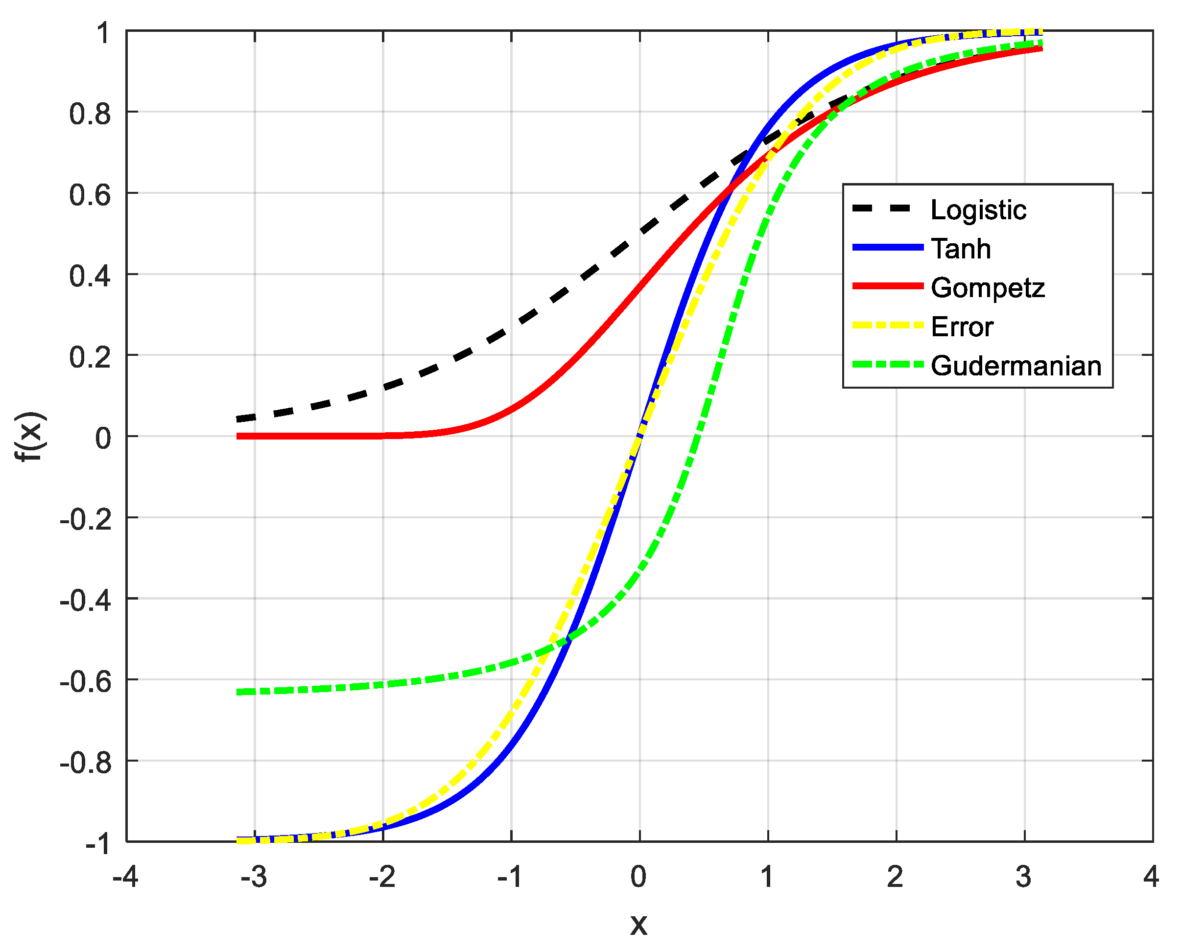
where five functions consisting of the hyperbolic tangent function, the logistic function, the gom function, the erf function and the gd function can be defined as follows:

$$logistic\left(x\right)=\frac{1}{1+e^{-x}}$$

(43)

$$tanh (x)=\frac{e^x-e^{-x}}{e^x+e^{-x}}$$

(44)

$$gom\left(x\right)=e^{-e^{-x}}$$

(45)

$$erf\left(x\right)=\frac{2}{\sqrt{\pi }}\underset{0}{\overset{x}{{\displaystyle \int }}}{e}^{-t^2}$$

(46)

$$gd (x)=2\arctan \left(e^x\right)-\frac{1}{2}\pi$$

(47)

In [32], only one function, tanh(σU_i) (where σ is the slope and U_i is the input of neurons), was used to determine output for continuous neurons. There were three curves plotted in [32] corresponding to three values of σ, which were 0.005, 0.01 and 100. In this paper, we used the function together with four other functions shown in Equations (43)–(47). As such, five curves are plotted in Figure 1 that correspond to the five functions in which x is varied from −π to π.

Due to the use of five different functions, the five HLN methods are defined as the HLN-LF (the HLN with the logistic function), the HLN-THF (the HLN with the hyperbolic tangent function), the HLN-GF (the HLN with the Gompertz function), the HLN-EF (the HLN with the error function) and the HLN-GdF (the HLN with the Gudermanian function). It should be noted that each function contains both the slope and input of neurons, and each function is used to calculate the output for the neurons shown in Equations (33)–(42). Then, these outputs and inputs are used to calculate the dynamics of the neurons shown in Equations (18)–(22) in the next iterations. In next step, the dynamics of neurons are used to update inputs for neurons. The steps are repeated until the maximum error is not higher than Tol_pre. Thus, the effectiveness of each function cannot be explained in theory, but using obtained results can illustrate their contribution to determine the output for neurons.

3.2. The Entire Search Process of the HLN

3.2.1. Selection of Parameters

In the HLN, there are many parameters need to be tuned. These parameters consist of

(1)

σ

(2)

α₁, α₂, α₃, α₄ and α₅

(3)

Predetermined tolerance Tol_pre

(4)

Maximum iteration G_max

Among the parameters, σ directly influences the outputs for continuous neurons as shown in Equations (33)–(42). There is no predetermined range for σ; however, the parameter can be set to the same value of 100 for all study cases, and the results are good enough for acceptance. α₁, α₂, α₃, α₄ and α₅ are set to small values which are higher than 0 but much smaller than 1. There is no rule for tuning the values of the five parameters excluding the trial and error method. For different study cases, these parameters are set to difference values. Tol_pre has a high impact on the quality of optimal solutions, and it can be tried by setting to 10⁻¹, 10⁻², 10⁻³, 10⁻⁴ and 10⁻⁵. When setting Tol_pre to a very small value, the convergence is hardly ever reached. However, a higher value can easily lead to convergence, but the objective function of the obtained solutions, i.e., total profit, cannot reach the maximum value as expected. However, the impact of Tol_pre on results when setting the range from 10⁻⁵ to 10⁻⁴ is insignificant—even the same. In contrast to the other parameters, G_max does not lead to good or bad results, but it is employed to control the convergence of the HLN. In the HLN, the termination condition is based on maximum error. However, in order to avoid loss of control, G_max can stop the iterative search process if the computational iteration is equal to G_max. In this case, the termination condition is not exactly satisfied. If the maximum error is less than Tol_pre, the computational iteration is smaller than G_max. As such G_max can be set to 5000 for all study cases.

3.2.2. Initialization

Inputs for both multiplier neurons and continuous neurons can be randomly produced within the range of 0–1. In addition, outputs for continuous neurons consisting of V_i,P and V_i,PR are randomly produced within the lower bound and the upper bound, while outputs for multiplier neurons consisting of $V_{\lambda },V_{\gamma }$ and $V_{i,\mu }^{}$ are randomly initialized between 0 and 1. The initialization can be summarized as follows:

$$U_{\lambda }=0+{\epsilon }_1(1-0)$$

(48)

$$U_{\gamma }=0+{\epsilon }_2(1-0)$$

(49)

$$U_{i,\mu }=0+{\epsilon }_3(1-0)$$

(50)

$$V_{\lambda }=0+{\epsilon }_4(1-0)$$

(51)

$$V_{\gamma }=0+{\epsilon }_5(1-0)$$

(52)

$$V_{i,\mu }=0+{\epsilon }_6(1-0)$$

(53)

$$P{R}_i^{\max }=P{R}_i^{\min }+{\epsilon }_7(P{R}_i^{\max }-P{R}_i^{\min })$$

(54)

$$P_i^{\max }=P_i^{\min }+{\epsilon }_8(P_i^{\max }-P_i^{\min })$$

(55)

where ε₁, ε₂, ε₃, ε₄, ε₅, ε₆, ε₇ and ε₈ are random numbers within the range from 0 to 1.

3.2.3. Condition of Computation Termination

The search procedure ends if the current iteration (G) is equal to the maximum iteration (G_max) or the maximum error (Error_max) is equal or smaller than predetermined tolerance (Tol_pre). For all cases, we set G_max = 5000 and Tol_pre = 10⁻⁴, and Error_max is determined by:

$$Erro{r}_P={\displaystyle \sum _{i=1}^N{V}_{i,P}}-P_D$$

(56)

$$Erro{r}_{PR}={\displaystyle \sum _{i=1}^N{V}_{i,PR}}-P{R}_D$$

(57)

$$Erro{r}_{PRi}=V_{i,PR}-P_i^{\max };i=1,\dots ,\mathrm{N}$$

(58)

$$Erro{r}_{\max }=\max \left\{Erro{r}_P,Erro{r}_{PR},\max \left(Erro{r}_{PRi}\right)\right\}$$

(59)

3.2.4. The Iterative Algorithm of the HLN for Dealing with the Considered Problem

The iterative algorithm of the HLN for solving the considered OLD problem in the competitive environment is given in Figure 2 and expressed by the following steps:

Step 1:

Set values for control parameters, as expressed in Section 3.2.1.

Step 2:

Randomly generate inputs as well as outputs for multiplier neurons and continuous neurons, as shown in Section 3.2.2.

Step 3:

Set current iteration G to 1.

Step 4:

Determine the dynamics of inputs and outputs for all neurons, as shown in Section 3.1.2.

Step 5:

Update the inputs for multiplier neurons and continuous neurons by using Section 3.1.3.

Step 6:

Update the outputs for multiplier neurons and continuous neurons by using Section 3.1.4.

Step 7:

Calculate individual error and maximum error, as shown in Section 3.2.2.

Step 8:

If Error_max > Tol_pre and G < G_max, set G = G + 1 and return to Step 3. Otherwise, stop the HLN and print results.

4. Numerical Results

In the section, we have implemented the HLN with five functions for updating the outputs for continuous neurons, as shown in Equations (33)–(42). For each study case, we executed each HLN method for 100 independent trial runs, and then the results in terms of the average profit, maximum profit, minimum profit, average of iterations and maximum error were reported. The iterative algorithms were coded in Matlab program language and run on a 2.40 GHz personal computer.

4.1. Three-Unit System

In this section, the HLN method is tested on the three-unit system shown in Figure 3 with two revenue models consisting of payment for power delivered and payment for reserve allocated [33]. The two cases have the same input data such as the forecasted power demand of 1100 MW, the forecasted power reserve of 100 MW, the spot price of 11.3 ($/MWh) and the probability of reserve P_a = 0.005. However, reserve price is different, i.e., three times the spot price for the first revenue model and 0.004 times the spot price for the second revenue model. For implementing PSO, DE and the CSA, we set the population and the maximum number of iterations to 5 and 500, respectively, while the other parameters for each method were set by the following selection:

• PSO: c₁ = 2.05 and c₂ = 2.05 [36]
• DE: Crossover factor CR = 0.2, 0.4, 0.6, 0.8 and mutation factor F = 0.2, 0.4, 0.6, 0.8, 1.0 [34]
• CSA: The probability of replacing old solution for mutation operation Pro = 0.2, 0.4, 0.6, 0.8, 1.0 [37]

For the first revenue model, the results obtained by five HLNs and the three methods together with the ALHN are reported in

Table 1. Comparison of results obtained for three-unit system with the first revenue model.

Method	Mean Error	Max. Profit ($/h)	Mean. Profit ($/h)	Min. Profit ($/h)	Mean Iterations	CPu Time (s)
HLN-EF	0.000078	1102.45	1102.45	1102.45	40	0.017
HLN-THF	0.000091	1102.45	1102.45	1102.45	59	0.02
HLN-GdF	0.000098	1102.45	1102.45	1102.449	142	0.06
HLN-GF	0.000098	1102.45	1102.449	1102.449	155	0.062
HLN-LF	0.000098	1102.45	1102.45	1102.449	161	0.069
PSO	0.000078	1102.45	938.8674	325	500	0.383
CSA	0.000091	1102.45	1099.229	1040.159	500	0.765
DE	0.000098	1102.45	635.3542	−111.923	500	0.808
ALHN [33]	-	1102.45	-	-	5000	0.16

.

The obtained results from the five HLN methods including maximum profit, mean profit, minimum profit, mean error, and mean iterations together with simulation time are shown in Table 1 and

Table 2. Comparison of results obtained for three-unit system with the second revenue model.

Method	Mean Error	Max. Profit ($/h)	Mean. Profit ($/h)	Min. Profit ($/h)	Mean Iterations	CPu Time (s)
HLN-EF	0.000097	1095.648	1095.648	1095.6474	173	0.07
HLN-THF	0.0001	1095.647	1095.647	1095.646	240	0.1
HLN-GdF	0.000099	1095.61	1095.61	1095.61	421	0.18
HLN-GF	0.000098	1095.589	1095.589	1095.5893	432	0.185
HLN-LF	0.000102	1095.59	1095.59	1095.589	413	0.32
PSO	-	1095.648	943.7049	232.7724	500	0.77
CSA	-	1095.648	1088.329	959.5354	500	0.82
DE	-	1095.648	745.1618	57.8145	500	0.95
ALHN [33]	-	1095.65	-	-	5000	0.16

for the first and the second revenue models, respectively. In addition, results from PSO, the CSA, DE and the ALHN [33] are also reported in the tables for comparison. Table 1 indicates that all methods had the same maximum profit for the first revenue model with 1102.45 ($/h), while the mean profit and the minimum profit of the proposed HLN were better than those of other methods excluding the ALHN because the ALHN used the same initial outputs for multiplier neurons and continuous neurons. These results mean that the five HLNs had the best stability, and approximately all runs had the same profit as the best run. In addition, the five HLN methods were also faster than other ones, since the mean iterations were from 40 to 161 and the simulation times of the HLN methods were the fastest from 0.017 to 0.069 s; the other methods used 500 iterations and took about 0.4–0.8 s. Similarly, the five HLN methods were better than other ones for the second revenue model. The maximum profit of all methods was approximately similar, but the mean and the minimum profits of the HLN methods were much higher. The observation of mean iterations and simulation times indicates that the HLN method could search optimal solutions much faster than other ones. Thus, it can be concluded that the HLN methods are the best methods among the applied methods.

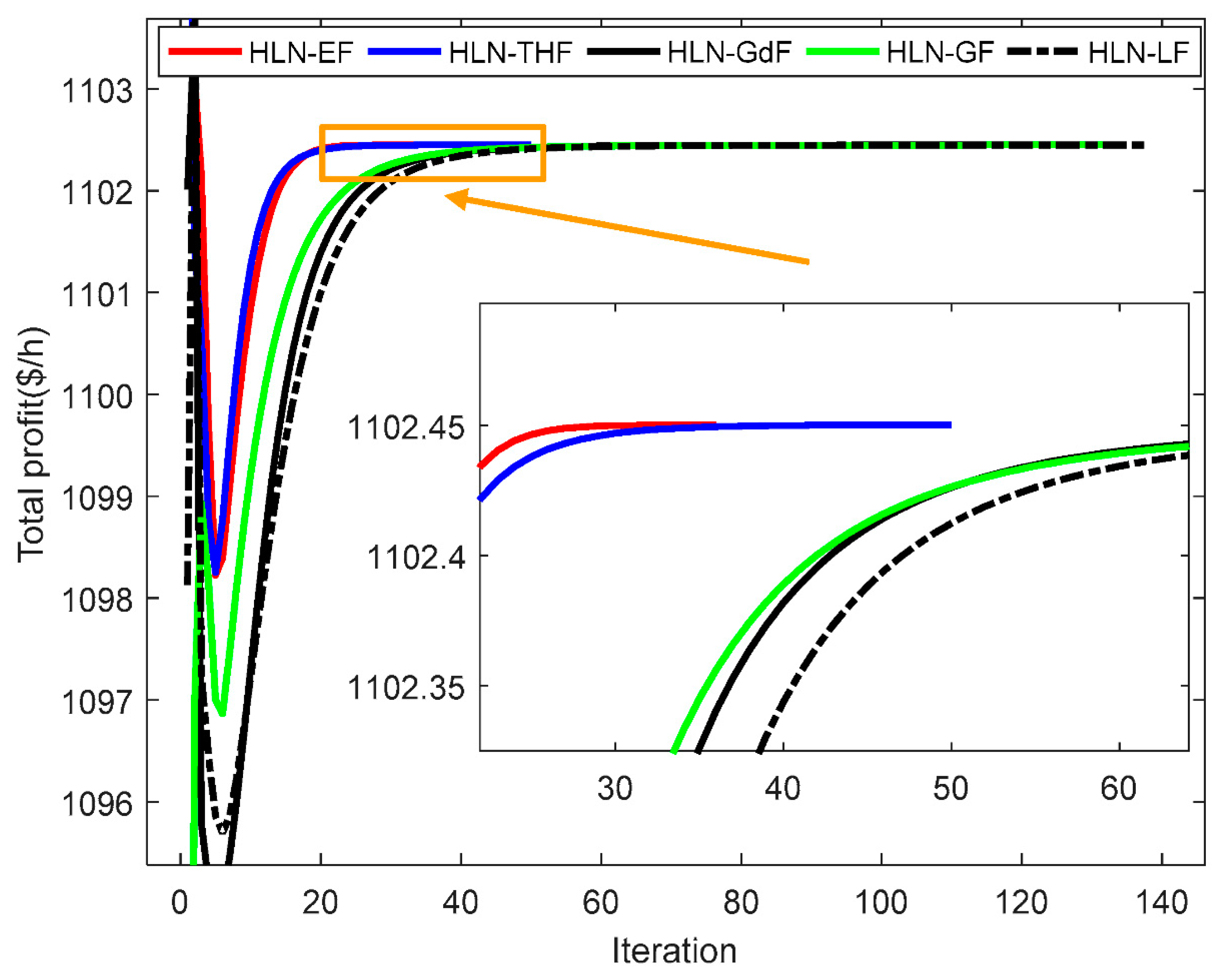
In comparison among the five HLN methods, it should be noted that the HLN-EF had the best performance because its mean error and mean iterations were the lowest. Its mean error was much smaller than Tol_pre for two cases, but those of other methods were slightly smaller or higher than Tol_pre. The mean errors were, respectively, 0.000078 and 0.000097 for the two cases, while Tol_pre was equal to 0.0001. The mean iterations of the HLN-EF were 40 and 173, but those of other methods were from 59 to 161 for the first case and from 240 to 432 for the second case. Figure 4 and Figure 5, respectively, show the maximum error and the profit at each computation iteration for the system with the first revenue model. These figures indicate that all HLN methods can stabilize the maximum error at each iteration since the fluctuations were nearly zero and the maximum error of the later iteration was lower than that of the previous iteration. For choosing the best method, the HLN-EF in red could reach the termination condition and the highest profit before the 40th iteration for the first model, whereas the other HLN methods were searching solutions, reducing the maximum errors and increasing total profits. The HLN-THF was the second best method for reaching the termination condition and the highest profit. Three remaining methods such as the HLN-GdF, the HLN-GF and the HLN-LF had the same manner in finding solutions, with about 140 iterations. The mean iterations shown in Table 1 also support this observation, since the three methods had the mean iterations higher than 150 iterations. Figure 6 and Figure 7, respectively, illustrate the maximum error and the profit over the search process for the system with the second revenue model. The two figures also provide good evidence for indicating the superiority of the HLN-EF over other methods, since the method reached the smallest error at about iteration 170, while other ones used about approximately 250 and 450 iterations. As such, it can be concluded that error function is the best model for the updating outputs for continuous neurons.

All of the data of the system and optimal solutions obtained by the HLN-EF for the system are shown in

Table A1. All of the data for the three-unit system.

Unit i	ci	bi	ai	${\mathit{P}}_{\mathit{i}}^{\mathbf{min}}\left(\mathbf{MW}\right)$	${\mathit{P}}_{\mathit{i}}^{\mathbf{max}}\left(\mathbf{MW}\right)$
1	0.002	10.000	500.000	100.000	600.000
2	0.0025	8.000	300.000	100.000	400.000
3	0.005	6.000	100.000	50.000	200.000

and

Table A2. All of the data for the 10-unit system.

Unit i	ci	bi	ai	${\mathit{P}}_{\mathit{i}}^{\mathbf{min}}\left(\mathbf{MW}\right)$	${\mathit{P}}_{\mathit{i}}^{\mathbf{max}}\left(\mathbf{MW}\right)$
1	0.0004800	16.19	1000	150	455
2	0.0003100	17.26	970	150	455
3	0.00200	16.60	700	20	130
4	0.0021100	16.50	680	20	130
5	0.0039800	19.70	450	25	162
6	0.0071200	22.26	370	20	80
7	0.0007900	27.74	480	25	85
8	0.0041300	25.92	660	10	55
9	0.0022200	27.27	665	10	55
10	0.0017300	27.79	670	10	55

of Appendix A.

4.2. Ten-Unit System

In this section, a 10-unit system which also had two revenue models was employed to run the HLN, PSO, DE and CSA methods. All of the data of the system were taken from [33]. The two cases had the same input data, such as a forecasted power demand of 1500 MW, a forecasted power reserve of 150 MW and a spot price of 31.65 ($/MWh). However, P_a and PRP were different for two models—P_a = 0.05 and PRP = 5 × PSP for the first model and P_a = 0.005 and PRP = 0.01 × PSP for the second model. For implementing PSO, DE and the CSA, we set the population and the maximum number of iteration to 10 and 500, respectively, while the other parameters for each method were set to the same values shown in section above. The results from the HLN and other methods are shown in

Table 3. Comparison of results obtained for the 10-unit system with the first revenue model.

Method	Mean Error	Max. Profit ($/MWh)	Mean Profit ($/MWh)	Min. Profit ($/MWh)	Mean Iterations	CPu Time (s)
HLN-EF	0.000095	14,564.731	14,564.73	14,564.729	194	0.08
HLN-THF	0.000095	14,564.73	14,564.73	14,564.727	225.6	0.1
HLN-GdF	0.000092	14,564.716	14,564.715	14,564.70	256.81	0.11
HLN-GF	0.000093	14,564.714	14,564.714	14,564.713	195	0.08
HLN-LF	0.000082	14,564.714	14,564.713	14,564.712	279.57	0.22
PSO	-	14,182.186	9771.186	836.9154	500	1.5
CSA	-	14,564.05	14,501.86	14,201.51	500	1.7
DE	-	14,053.027	8416.1628	2281.539	500	1.9
ALHN [33]	-	14,564.73	-	-	5000	0.18

and

Table 4. Comparison of results obtained for the 10-unit system with the second revenue model.

Method	Mean Error	Max. Profit ($/MWh)	Mean Profit ($/MWh)	Min. Profit ($/MWh)	Mean Iterations	CPu Time (s)
HLN-EF	0.000092	13,635.1083	13,635.1083	13,635.1083	187	0.08
HLN-THF	0.000084	13,635.1082	13,635.1081	13,635.1078	227.56	0.1
HLN-GdF	0.000088	13,635.1061	13,635.106	13,635.105	270.48	0.12
HLN-GF	0.000091	13,635.1067	13,635.1061	13,635.1059	195	0.09
HLN-LF	0.000085	13,635.1059	13,635.1058	13,635.105	278.86	0.22
PSO	-	13,158.0653	9824.8414	6246.4383	500	1.6
CSA	-	13,635.105	13,448.0525	13,177.6998	500	1.7
DE	-	13,093.1919	8346.2441	3729.7168	500	2.0
ALHN [33]	-	13,635.11	-	-	5000	0.18

for two cases. For the first case, the maximum profit from the HLN methods was approximately equal to the best value of 14,564.731 $/h and was the highest value among all compared. The mean profit and the lowest profit of the HLN methods were nearly equal to the maximum profit and much higher than those from the PSO, CSA and DE methods. In fact, the highest profits of the three methods were, respectively, 14,182.186, 14,564.05 and 14,053.027 $/h. Meanwhile, their lowest profits were, respectively, 836.9154, 14,201.51, and 2281.539. Similarly, the maximum profit and the minimum profit of the proposed HLN methods were nearly alike and equaled 13,635.1081 $/h for the second case, but those of PSO, the CSA and DE were much worse. Their best profits were 13,158.0653, 13,635.105, and 13,093.1919 $/h, and their worst profits were 6246.4383, 13,177.6998, and 3729.7168 $/h, respectively. Furthermore, the execution time from the HLN methods was much shorter than those of the other methods. It was around 0.1 s for the HLN methods, but it was about 2.0 s for other ones, excluding the ALHN. Clearly, the HLN methods are much more effective for a large-scale system.

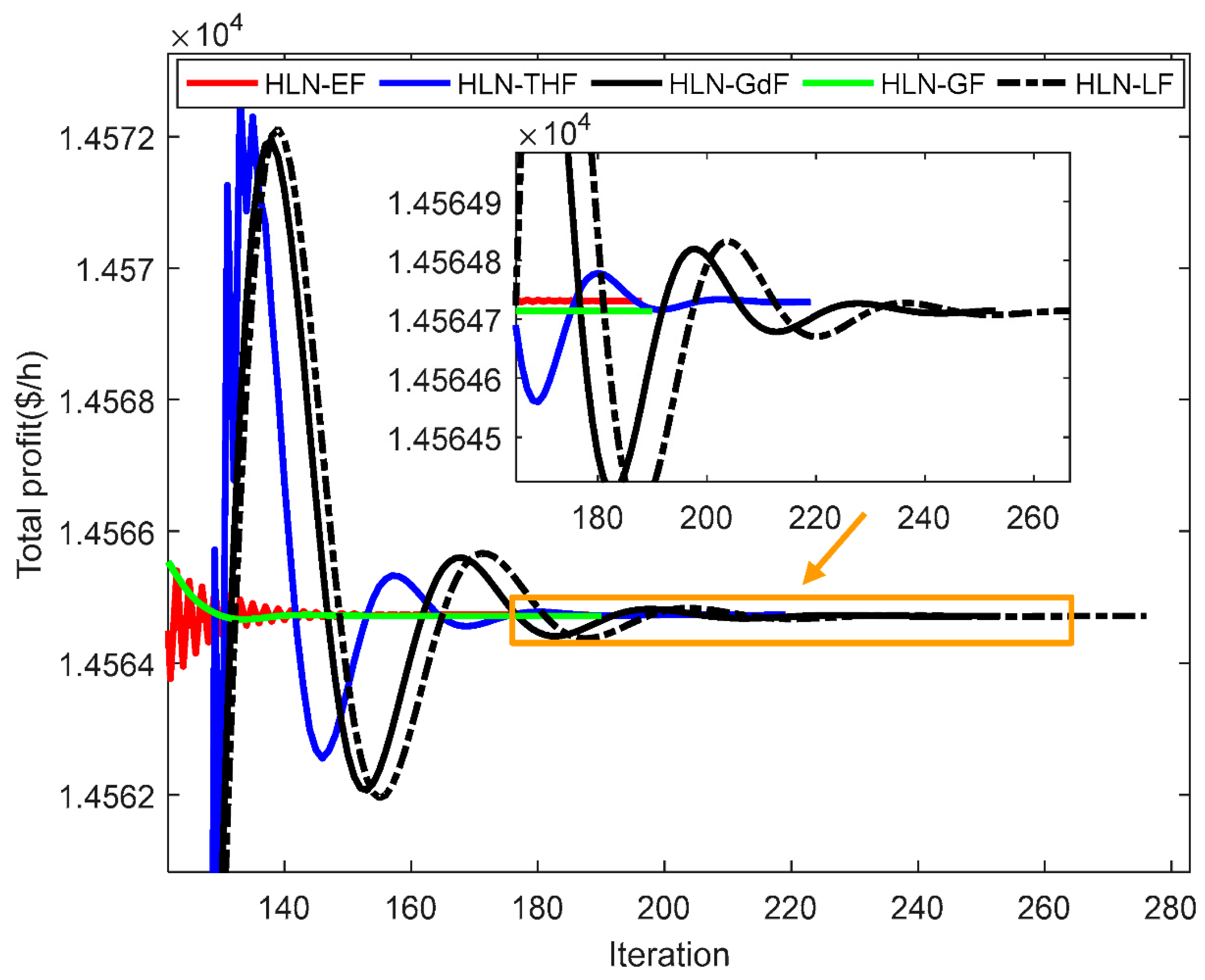
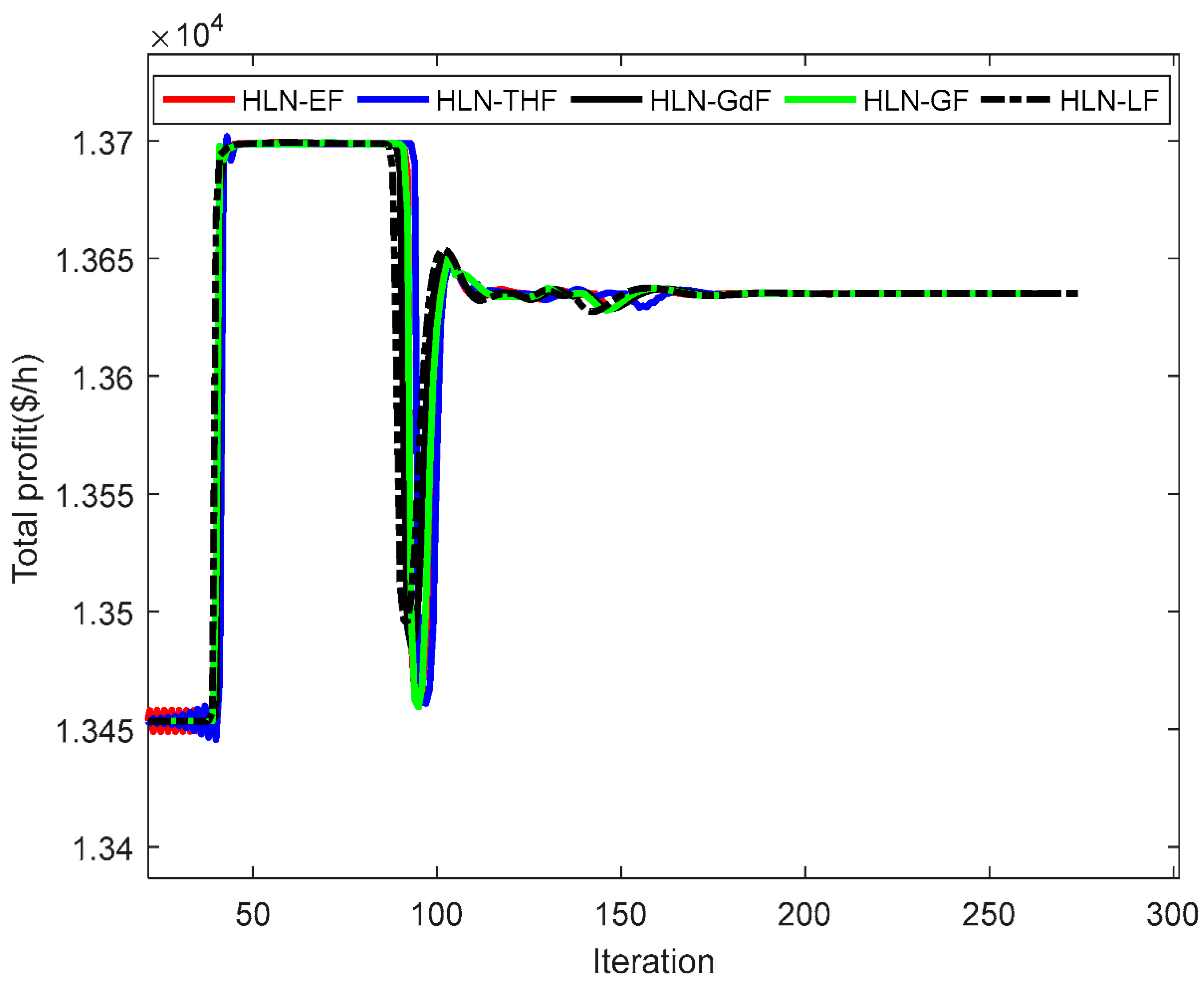
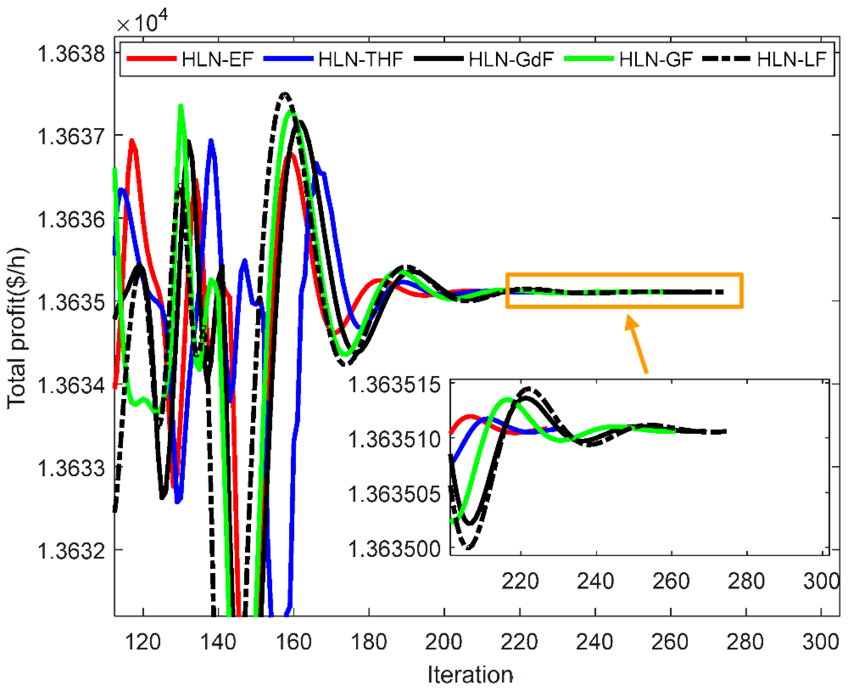
Comparison among the five HLN methods had the same evaluation as the first system with three units. The HLN-EF was the best one with the highest maximum profit and minimum profit. In addition, the iteration from the HLN-EF was the smallest for two cases. Figure 8 show a whole view of search process for finding optimal solutions by using the first model of the revenue. As seen from this figure, these applied methods could not stabilize the maximum error over the whole search process. The maximum errors fluctuated from the 10th iteration to the 50th iteration, and then the fluctuation decreased and kept decreasing until the final iteration was reached. However, a clear view for observing the decrease of the maximum error cannot be presented in Figure 8. Therefore, Figure 9 was plotted for zooming in Figure 8 from the 120th iteration to the last iteration. Observing the five curves can see that the HLN-EF (in red) and the HLN-GF (in green) could reach the smallest fluctuations and the smallest maximum error; however, the HLN-EF was always better and reached the convergence first. The HLN-GdF and the HLN-LF (in black) were the two worst methods with the highest fluctuations and the highest maximum error. The HLN-THF (in blue) was separated into a group. Corresponding to the view of the maximum error, the view of the total profit can be seen by the meaning of Figure 10 and Figure 11, where Figure 11 is plotted for zooming in Figure 10 from the 120th iteration to the last iteration. Figure 10 also has the same fluctuation as Figure 8 for the first fifty iterations, and the fluctuations decreased after the 50th iteration. However, the entire view of Figure 10 cannot show the clear stabilization of the total profit. Figure 11 indicates that the HLN-EF (in red) could reach the highest profit and stopped searching for new solutions at about the 180th iteration, while the HLN-GF (in green) found the second best profit after about two iterations. The three remaining methods still got a stable profit and reached maximum profit after the 200th iteration. Clearly, Figure 8, Figure 9, Figure 10 and Figure 11 give good evidence for the outstanding performance of the HLN-EF over other ones for the first model. Similarly, the best performance of the HLN-EF for the second model of the system with 10 units can be observed by plotting Figure 12, Figure 13, Figure 14 and Figure 15. The whole view of the maximum error and the total profit is presented in Figure 12 and Figure 14, while Figure 13 and Figure 15 zoom in Figure 12 and Figure 14 for better views of search process. Figure 12 and Figure 14 show the fluctuations of maximum error and total profit last from the first iteration to the 150th iteration; the fluctuations decreased dramatically until the last iteration was reached. Figure 13 and Figure 15 point out the best performance of the HLN-EF in red and the second best performance of the HLN-THF in blue because the two methods stopped searching at about the 230th iteration with the highest profit, whereas other ones were still searching for solutions and increasing total profit. Consequently, it can be concluded that error function is the most appropriate function for updating the outputs for continuous neurons.

All of the data of the system and optimal solutions obtained by the HLN-EF for the system are shown in

Table A3. Optimal solutions for the three-unit system obtained by HLN-EF.

i	Case 1		Case 2
	Pi (MW)	PRi (MW)	Pi (MW)	PRi (MW)
1	324.8165	99.9999	324.8165	99.9958
2	400	0	400	0
3	200	0	200	0

and

Table A4. Optimal solutions for the 10-unit system obtained by HLN-EF.

i	Case 1		Case 2
	Pi (MW)	PRi (MW)	Pi (MW)	PRi (MW)
1	455	0	455.0000	0
2	455	0	455.0000	0
3	130	0	130.0000	0
4	130	0	130.0000	0
5	162	0	162.0000	0
6	80	0	80.0000	0
7	25	55.3590	25.0000	54.8954
8	43	12.0001	43.0001	12.0000
9	10	44.9669	10.0000	42.2942
10	10	37.6740	10.0000	40.8105

of Appendix A.

4.3. Discussion on the HLN with Different Applied Functions

As can be seen in Table 1 and Table 2 for the first system with three units, the HLN methods had approximately the same maximum profit. For the first model, all HLN methods could find the same profit of $1102.45, but for the second model, only the HLN-EF could find $1095.648—the other ones reached less profit. However, the deviation was not high. This means that all applied functions could support the HLN to find the best performance for the system. However, the number of iterations and the mean profit of all runs indicate that the HLN-EF is the best one because its mean and its maximum were equal. As seen from Table 3 and Table 4, the phenomenon was nearly repeated for the second systems, and the HLN-EF was still the best method among the five HLN methods. However, the mean iterations from these study cases were different. The HLN-EF reached the smallest number of iterations (40 iterations) for the first model of the first system, while the mean iterations were higher for the second system because the second system was comprised of 10 units. In this study, we set many parameters to random values such as the inputs and outputs for the Lagrange multiplier neurons, and the power output and the power reserve of all units as shown in Equations (48)–(55). The setting and the simulation results mean that applications of the HLN methods are not dependent on the initial parameters that the ALHN in [33] suffered. By comparing all the HLN methods to PSO, DE and the CSA, it can be seen that the maximum profits indicated that the HLN methods were much more effective than these methods for the second system with 10 units, while the mean of profit over 100 runs indicated that the HLN methods were more stable in finding optimal solutions. This also shows that that the HLN methods were not influenced by the randomization factors that PSO, the CSA and DE had to suffer.

5. Conclusions

In this paper, we proposed five HLN methods for solving the OLD problem while considering the electricity market and complex constraints. Five functions consisting of the logistic, hyperbolic tangent, Gompertz, error and Gudermanian functions were employed to establish five HLN methods. Two systems with three and ten units were employed for two revenue models to run the HLN methods, with the CSA, PSO and DE methods being used for comparison. The comparisons of maximum profit indicated that the HLN methods could reach the same optimal solution as other methods for the first system, but they could reach much better solution for larger system with ten units. The proposed HLN methods were also more stable and faster than other ones since they had a better mean profit, a better minimum profit, lower iterations and faster simulation times for the two systems. Thus, the HLN methods were superior to other compared methods. Among the five applied HLN methods, the HLN-EF with the use of error function was the best method, since the maximum profit, mean profit and minimum profit of all runs were approximately equal for two considered systems with two models of revenue. In addition, the HLN-EF reduced the maximum error and reached the highest profit fastest with the smallest number of iterations. Furthermore, the whole view of search process from the two systems indicated that the HLN-EF had the smallest fluctuations of maximum error and maximum profit, and it reached termination condition fastest. Consequently, it is recommended that the HLN and error function should be tried for other optimization problems in electrical engineering.

In this problem, with the consideration of the electric market, we have considered different prices for power produced and reserved from thermal generating units. Nowadays, electricity from solar or wind systems accounts for a high rate from all power sources [38,39]. As such, a consideration of renewable energies can be a good research field in optimizing load dispatch in the electric market. If all renewable energies can be joined in the electric market, power systems can become more stable and effective.

References

- Nguyen, T.T.; Nguyen, C.T.; Van Dai, L.; Vu Quynh, N. Finding Optimal Load Dispatch Solutions by Using a Proposed Cuckoo Search Algorithm. Math. Probl. Eng. 2019. [Google Scholar] [CrossRef]
- Jeyakumar, D.N.; Jayabarathi, T.; Raghunathan, T. Particle swarm optimization for various types of economic dispatch problems. Int. J. Electr. Power Energy Syst. 2006, 28, 36–42. [Google Scholar] [CrossRef]
- Noman, N.; Iba, H. Differential evolution for economic load dispatch problems. Electr. Power Syst. Res. 2008, 78, 1322–1331. [Google Scholar] [CrossRef]
- Walters, D.C.; Sheble, G.B. Genetic algorithm solution of economic dispatch with valve point loading. IEEE Trans. Power Syst. 1993, 8, 1325–1332. [Google Scholar] [CrossRef]
- Nguyen, T.T.; Vo, D.N. The application of one rank cuckoo search algorithm for solving economic load dispatch problems. Appl. Soft Comput. 2015, 37, 763–773. [Google Scholar] [CrossRef]
- Nguyen, T.; Vo, D.; Vu Quynh, N.; Van Dai, L. Modified cuckoo search algorithm: A novel method to minimize the fuel cost. Energies 2018, 11, 1328. [Google Scholar] [CrossRef]
- Pham, L.H.; Duong, M.Q.; Phan, V.D.; Nguyen, T.T.; Nguyen, H.N. A High-Performance Stochastic Fractal Search Algorithm for Optimal Generation Dispatch Problem. Energies 2019, 12, 1796. [Google Scholar] [CrossRef]
- Kien, L.C.; Nguyen, T.T.; Hien, C.T.; Duong, M.Q. A Novel Social Spider Optimization Algorithm for Large-Scale Economic Load Dispatch Problem. Energies 2019, 12, 1075. [Google Scholar] [CrossRef]
- Ghasemi, M.; Taghizadeh, M.; Ghavidel, S.; Abbasian, A. Colonial competitive differential evolution: An experimental study for optimal economic load dispatch. Appl. Soft Comput. 2016, 40, 342–363. [Google Scholar] [CrossRef]
- Adarsh, B.R.; Raghunathan, T.; Jayabarathi, T.; Yang, X.S. Economic dispatch using chaotic bat algorithm. Energy 2016, 96, 666–675. [Google Scholar] [CrossRef]
- Kong, X.Y.; Chung, T.S.; Fang, D.Z.; Chung, C.Y. An power market economic dispatch approach in considering network losses. In Proceedings of the IEEE Power Engineering Society General Meeting, San Francisco, CA, USA, 16 June 2005; pp. 208–214. [Google Scholar] [CrossRef]
- Richter, C.W.; Sheble, G.B. A profit-based unit commitment GA for the competitive environment. IEEE Trans. Power Syst. 2000, 15, 715–721. [Google Scholar] [CrossRef]
- Shahidehpour, M.; Marwali, M. Maintenance Scheduling in Restructured Power Systems; Springer Science Business Media: Berlin, Germany, 2012. [Google Scholar]
- Hermans, M.; Bruninx, K.; Vitiello, S.; Spisto, A.; Delarue, E. Analysis on the interaction between short-term operating reserves and adequacy. Energy Policy 2018, 121, 112–123. [Google Scholar] [CrossRef]
- Allen, E.H.; Ilic, M.D. Reserve markets for power systems reliability. IEEE Trans. Power Syst. 2000, 15, 228–233. [Google Scholar] [CrossRef]
- Attaviriyanupap, P.; Kita, H.; Tanaka, E.; Hasegawa, J. A hybrid LR-EP for solving new profit-based UC problem under competitive environment. IEEE Trans. Power Syst. 2003, 18, 229–237. [Google Scholar] [CrossRef]
- Chandram, K.; Subrahmanyam, N.; Sydulu, M. New approach with muller method for profit based unit commitment. In Proceedings of the 2008 IEEE Power and Energy Society General Meeting-Conversion and Delivery of Electrical Energy in the 21st Century, Pittsburgh, PA, USA, 20–24 July 2008; pp. 1–8. [Google Scholar] [CrossRef]
- Ictoire, T.A.A.; Jeyakumar, A.E. Unit commitment by a tabu-search-based hybrid-optimisation technique. IEE Proc.-Gener. Transm. Distrib. 2005, 152, 563–574. [Google Scholar] [CrossRef]
- Dimitroulas, D.K.; Georgilakis, P.S. A new memetic algorithm approach for the price based unit commitment problem. Appl. Energy 2011, 88, 4687–4699. [Google Scholar] [CrossRef]
- Columbus, C.C.; Simon, S.P. Profit based unit commitment: A parallel ABC approach using a workstation cluster. Comput. Electr. Eng. 2012, 38, 724–745. [Google Scholar] [CrossRef]
- Columbus, C.C.; Chandrasekaran, K.; Simon, S.P. Nodal ant colony optimization for solving profit based unit commitment problem for GENCOs. Appl. Soft Comput. 2012, 12, 145–160. [Google Scholar] [CrossRef]
- Sharma, D.; Trivedi, A.; Srinivasan, D.; Thillainathan, L. Multi-agent modeling for solving profit based unit commitment problem. Appl. Soft Comput. 2013, 13, 3751–3761. [Google Scholar] [CrossRef]
- Singhal, P.K.; Naresh, R.; Sharma, V. Binary fish swarm algorithm for profit-based unit commitment problem in competitive electricity market with ramp rate constraints. IET Gener. Trans. Distrib. 2015, 9, 1697–1707. [Google Scholar] [CrossRef]
- Sudhakar, A.V.V.; Karri, C.; Laxmi, A.J. A hybrid LR-secant method-invasive weed optimisation for profit-based unit commitment. Int. J. Power Energy Convers. 2018, 9, 1–24. [Google Scholar] [CrossRef]
- Reddy, K.S.; Panwar, L.K.; Panigrahi, B.K.; Kumar, R. A New Binary Variant of Sine–Cosine Algorithm: Development and Application to Solve Profit-Based Unit Commitment Problem. Arab. J. Sci. Eng. 2018, 43, 4041–4056. [Google Scholar] [CrossRef]
- Reddy, K.S.; Panwar, L.; Panigrahi, B.K.; Kumar, R. Binary whale optimization algorithm: A new metaheuristic approach for profit-based unit commitment problems in competitive electricity markets. Eng. Optim. 2019, 51, 369–389. [Google Scholar] [CrossRef]
- Gonidakis, D.; Vlachos, A. A new sine cosine algorithm for economic and emission dispatch problems with price penalty factors. J. Inf. Optim. Sci. 2019, 40, 679–697. [Google Scholar] [CrossRef]
- Liang, H.; Liu, Y.; Li, F.; Shen, Y. A multiobjective hybrid bat algorithm for combined economic/emission dispatch. Int. J. Electr. Power Energy Syst. 2018, 101, 103–115. [Google Scholar] [CrossRef]
- Rezaie, H.; Abedi, M.; Rastegar, S.; Rastegar, H. Economic emission dispatch using an advanced particle swarm optimization technique. World J. Eng. 2019. [Google Scholar] [CrossRef]
- Mason, K.; Duggan, J.; Howley, E. A multi-objective neural network trained with differential evolution for dynamic economic emission dispatch. Int. J. Electr. Power Energy Syst. 2018, 100, 201–221. [Google Scholar] [CrossRef]
- Bora, T.C.; Mariani, V.C.; dos Santos Coelho, L. Multi-objective optimization of the environmental-economic dispatch with reinforcement learning based on non-dominated sorting genetic algorithm. Appl. Therm. Eng. 2019, 146, 688–700. [Google Scholar] [CrossRef]
- Vo, D.N.; Ongsakul, W. Hopfield lagrange network for economic load dispatch. Innov. Power Control. Optim. 2012, 57–94. [Google Scholar] [CrossRef]
- Vo, D.N.; Ongsakul, W.; Nguyen, K.P. Augmented Lagrange Hopfield network for solving economic dispatch problem in competitive environment. AIP Conf. Proc. 2012, 1499, 46–53. [Google Scholar] [CrossRef]
- Nguyen, T.; Vu Quynh, N.; Duong, M.; Van Dai, L. Modified differential evolution algorithm: A novel approach to optimize the operation of hydrothermal power systems while considering the different constraints and valve point loading effects. Energies 2018, 11, 540. [Google Scholar] [CrossRef]
- Nguyen, T.T. Solving Economic Dispatch Problem with Piecewise Quadratic Cost Functions Using Lagrange Multiplier Theory; International Conference Computer Technology Development ASME Press: New York, NY, USA, 2011; pp. 359–363. [Google Scholar] [CrossRef]
- Nguyen, T.T.; Vo, D.N. Improved particle swarm optimization for combined heat and power economic dispatch. Scientia Iranica. Trans. D Comput. Sci. Eng. Electr. 2016, 23, 1318. [Google Scholar] [CrossRef]
- Nguyen, T.T.; Nguyen, T.T.; Vo, D.N. An effective cuckoo search algorithm for large-scale combined heat and power economic dispatch problem. Neural Comput. Appl. 2018, 30, 3545–3564. [Google Scholar] [CrossRef]
- Guo, C.; Wang, D. Frequency Regulation and Coordinated Control for Complex Wind Power Systems. Complexity 2019. [Google Scholar] [CrossRef]
- Gammoudi, R.; Brahmi, H.; Dhifaoui, R. Estimation of Climatic Parameters of a PV. System Based on Gradient Method. Complexity 2019. [Google Scholar] [CrossRef]
Figure 1.
Five applied functions for updating outputs of continuous neurons.
Figure 2.
The flowchart of using the Hopfield Lagrange network (HLN) for solving the considered problem.
Figure 3.
The first system with three units.
Figure 4.
Maximum error vs. iteration for the first system with the first model of payment.
Figure 5.
Total profit for the first system with the first model of payment.
Figure 6.
Maximum error vs. iteration for the first system with the second model of payment.
Figure 7.
Total profit for the first system with the second model of payment.
Figure 8.
Maximum error vs. iteration for the second system with the first model of payment.
Figure 9.
Zoom-in of Figure 8 from iteration 120 to the last iteration.
Figure 10.
Total profit for the second system with the first model of payment.
Figure 11.
Zoom-in of Figure 10 from iteration 120 to the last iteration.
Figure 12.
Maximum error vs. iteration for the second system with the second model of payment.
Figure 13.
Zoom-in of Figure 12 from iteration 115 to the last iteration.
Figure 14.
Total profit for the second system with the second model of payment.
Figure 15.
Zoom-in of Figure 14 from iteration 115 to the last iteration.