Computationally Efficient Method of Co-Energy Calculation for Transverse Flux Machine Based on Poisson Equation in 2D


Department of Electrical and Computer Engineering, Rzeszow University of Technology, 35-021 Rzeszow, Poland
*
Author to whom correspondence should be addressed.
†
These authors contributed equally to this work.
Energies 2019, 12(22), 4340; https://doi.org/10.3390/en12224340
Submission received: 16 October 2019
/
Revised: 5 November 2019
/
Accepted: 13 November 2019
/
Published: 14 November 2019
(This article belongs to the Special Issue Applied Energy System Modeling 2018)
Abstract
:The article presents an original method for numerical determination of the value of magnetic co-energy of a transverse construction motor. The aim of the developed method is initial determination of the co-energy value for the analyzed structure in the function of rotor rotation angle. The main requirement set to the presented method was the lowest possible complexity of the process computation, lack of the necessity to apply costly dedicated software, as well as creating construction 3D models. These requirements were met by applying specific cross-section/development of the analyzed machine geometry, as well as application of specific boundary conditions, which enabled reduction of the analyzed problem to solving a Poisson equation in 2D. The calculations were done with the Finite Element Method.
1. Introduction
Machines of transverse structure are gaining increasing popularity in various applications. The interests of science and industry focus, among others, on applications of this type of solutions in generator operation with wind turbines, in which they comprise an interesting alternative to solutions with Axial Flux Permanent Magnet (AFPM) machines [1]. Various approaches to the issue of computational aided design process of this type of generators were suggested in references. In the work of [2] analytic methods of determining generator electric properties were discussed, their accuracy was verified by means of measurement experiments of a machine prototype, in a smaller scale. The works of [3,4] present a different approach, in which in order to determine electric parameters of the studied machine the static analysis and dynamic three-dimensional Finite Element Method (FEM 3D) analysis are applied. In the aforementioned works the influence of several selected parameters and machine structure details on the values of leakage stream and the shape of the back electromotive force (EMF) induced voltage waveform was analyzed. The structure of Transverse Flux Machine (TFM) type generator analysis, in terms of its application in cooperation with a wind turbine, was also done in the approach that makes use of an equivalent magnetic circuit, the effects of which were described in [5]. Electric machines of transverse magnetic flow comprise an important research area for manufacturers of electric and hybrid cars [6]. Due to their reliability [7] and significantly better ratio of geometric dimensions to the achieved mechanical power they are an alternative to AFPM type constructions [8]. A wide range of applications results in emergence of numerous modifications of the construction [9,10,11] and faces the process of aided design of this type of machines with high demands. Due to their construction, the problems typical for TFM machines are high values of leakage flux [12] and relatively low values of power coefficient [13]. Moreover, due to compact structure, which is an advantage, such machines are susceptible to overheating, which may result in accelerated degradation of permanent magnets [14]. Development of the method of numerical aided design of the machines concerns most often the mechanical properties of the machine being designed, i.e., the achieved mechanical power, the developed torque and its conservation in transient states. It is based on cyclic determination of co-energy value of the machine being designed, in the function of rotor rotation angle, for current values of decision variables, in the process of computational optimization. Determination of co-energy values requires specifying magnetic field distribution in the machine, for rotor positions variable within the range of full electric angle. Due to the fact that electromagnetic torque generated by the machine comprises a derivative from its co-energy after rotation angle, in order to accurately determine the objective function value formulated in terms of obtaining the desired machine dynamic properties, the calculations of co-energy should be done with a small angular step. This situation causes that the task of numerical aided design of TFM type machines is, in terms of dynamic properties, an issue of very high computational complexity, especially when FEM 3D is applied to determine magnetic field distribution. The references include papers that present different approaches to decreasing computational complexity of the numerical aided design process of the machines with permanent magnets [15,16]. in references [17,18,19,20,21]. The results of the analyses done with the two-dimensional Finite Element Method (FEM 2D) for the TFM type machines were presented and discussed. The article also presents the method for determining the co-energy value of the machine of transverse flow of magnetic field, based on a 2D model. An original method of reflecting TFM machine geometry in a 2D model, as well as a computational procedure based on FEM that allows for accurate reflection of magnetic field distribution, were also presented. The obtained results were compared with the results of calculations done with the FEM 3D method in Ansys/Maxwell environment.
2. Description of the Method for Creating a Machine 2D Model
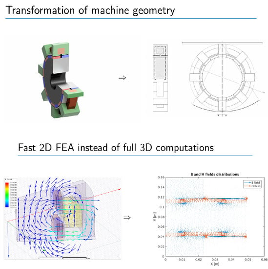
A view of a three-dimensional model of one phase of a machine of transverse flow of a magnetic field is presented in Figure 1. Permanent magnets are placed on rotor’s surface in such a way that magnetization vectors of magnets that comprise a pair are directed in opposite directions. Stator yoke that encompasses phase winding coil was marked with green color. In the space between consecutive stator yokes, over permanent magnets, there are high magnetic permeability elements.
The analysis of the presented machine geometry indicates that there is no possibility to reflect the studied type machine with a 2D model, by doing a simple cross-section. For this reason, only 3D (most often FEM) approach was applied in references to determine magnetic field distribution in constructions of this type. A method of creating a 2D model reflecting machine geometric properties in a sufficient way to do calculations of magnetic co-energy is presented below. Figure 1 presents a plane of a cross-section that goes through parts of machine stator and rotor on the way on which the flow of magnetic field closes. The field comes from both permanent magnets placed on machine rotor, as well as from the stator phase winding coil. To accurately determine the value of magnetic co-energy in the studied machine it is necessary to determine magnetic field distribution, considering both sources at the same time. Thus, in a 2D model it is necessary to:
- Reflect ways on which the magnetic field closes in a studied machine for one phase it is 8 systems that comprise of a pair of permanent magnets, stator yoke, as well as rotor parts (see Figure 1)
- provide a possibility to consider the presence of magnetic field that comes from stator winding phase coil current
To create a 2D model presenting the ways of magnetic field flow in a system, presented in Figure 1, the system was transformed to a 2D model by making a cross-section with simultaneous development of the geometry to a 2D system. This process is presented in Figure 2. A semi-view, semi-cross-section of a machine single pole pitch, with a marked cut line is presented on the left. A front view with a marked direction of geometry development to a 2D system is presented on the right.
The effect of this action is development of a 2D model, reflecting a one phase system of the studied machine in a way that enables us to determine magnetic field distribution coming from permanent magnets. According to the adopted assumptions the developed calculation method is aimed at creating the possibility to determine machine co-energy without the necessity to use any dedicated software, so all computation procedures were written from scratch in MATLAB environment, while the 2D model was prepared in AutoCad environment as a *.dxf file and imported to MATLAB. The diagram illustrating obtained 2D model of whole single-phase system is presented in Figure 3. The single pole pitch which is adopted as a 2D model for further analysis is marked witch a red box.
It should be noted that in a 2D model presented in Figure 3 the phase winding coil is not considered. The presence of the magnetic field coming from the current of this coil may be, however, considered in magnetostatic computations done for this model by providing a proper boundary condition. This is to be discussed in the following section. Due to the symmetries of the presented model all computations were done on the distance encompassing a machine single pole pitch, thus 1/8 of the full model of one phase (marked with a red box in Figure 3).
3. Description of the Computational Problem
Computation of magnetic field distribution in the studied machine to determine the value of co-energy is an issue of magnetostatics and comes down to a solution of Poison’s equation formulated for this problem in 2D space. This equation is solved regarding vector potential , defined so that:
where is the magnetic field induction vector.
Thus, the basic formula describing the analyzed problem has the following form:
where:
- —stator phase winding current,
- —equivalent magnetizing current
- —magnetic field strength vector
The presence of a permanent magnet may be represented by an equivalent current flowing in equivalent winding designed so that it goes through the model plane at straight angle on vertical edges of the permanent magnet. Then, by adopting the assumption that the width of equivalent winding tends to zero, the Equation 2 may be written as:
where is remanence vector of the permanent magnet, directed in accordance with the direction of magnetic field vector, generated by current in the equivalent winding. Then it is necessary to make Galerkin’s weak formulation for the analyzed problem. By introducing variances of vector potential we get:
Then, to transfer rotation operation from the element into a variance of vector potential by using the identity [22] we get:
Additionally, due to the geometry of the studied model it is justified to assume that the summary distribution of the magnetic field through the boundary of the studied area is zero. This implies the following dependence:
By taking the above into consideration and applying right transformations one gets a formula describing magnetic field distribution in the analyzed machine model, in the form that enables direct implementation of computation procedures of FEM 2D.
In FEM 2D computations the triangular elements with linear basis functions have been applied. The open source package provided in [23] was used for mesh generation. The overall procedure of formulation and solving a system of FEM. equations is described in detail in: [24,25,26,27,28,29]. The details of computational procedure are presented in [30].
4. Imposition of a Boundary Condition
4.1. Requirements Concerning the Imposed Boundary Conditions
It is necessary to note that in the developed 2D model of the TFM type machine, upper and bottom boundaries of the area correspond to the average central part of stator yoke. Thus, a part of the bottom boundary represents, together with the part of an upper boundary located opposite, one area that passes a three-dimensional system through middle parts of central stator yokes. It is expected that the magnetic field should be able to flow, in a free manner, through these boundaries. Taking into consideration the dependence 1, in the first approach it seems justified to introduce Neumann zero condition on upper and bottom boundaries. Such an approach introduces, however, excessive and ineligible limitation for the magnetic field flow through area boundaries, as it causes that the tangential component of vector on the area boundary has a value of zero. It is an excess limitation as it does not necessarily occur for the whole upper and bottom boundary. To eliminate this limitation, while providing free flow of magnetic field through upper and bottom boundaries, a boundary condition was formulated, which ensures that the difference of values of the vector potential between the nod at the beginning (calculating from the left) of the bottom boundary area and any other nod located in the bottom area boundary is equal to the difference of potentials at the upper boundary in nods that correspond, in terms of location, to pairs of bottom boundary nods. As mentioned before, to decrease computation complexity, the symmetry of the obtained 2D model was used. All computations were done on the fragment encompassing one pole pitch of the machine model, such approach requires consideration of this symmetry by means of imposing on vertical boundaries a model that corresponds to the appropriate boundary condition. In a typical example this condition works out to force that solution values obtained for given points on the left boundary are equal to the values obtained for corresponding points on the right boundary. In the discussed case of doing computations for a 2D model of the TFM type machine, this condition was modified in such a way that apart from the symmetry it considered the presence of a constant given value of the difference in values of the vector potential between the corresponding (in terms of location in the Y direction) points on the left and right boundaries. Such action forces the occurrence of magnetic field B in the direction of Y. In this way it is possible to consider, in the presented machine 2D model, the magnetic field stream that comes from phase winding coil current. Due to the fact that in the presented computation method the occurrence of the magnetic field saturation is not considered, the relation between phase winding coil current intensity and the difference of vector potential imposed in order to consider the presence of magnetic field stream, which is caused by this current, may be determined in the following way. For any imposed value of the difference of vector potential between the boundaries, the corresponding current of stator phase coil is calculated as an integral of magnetic field intensity on the closed curve that encompasses the coil. In a 2D model the curve corresponds to a straight line, which is parallel to Y direction and passes through the whole model in the place of stator yoke.
Then, by applying the assumed linear relationship between the values of current and magnetic field intensity, the value of the difference in vector potentials that corresponds to the current of unit intensity is determined.
4.2. The Method of Imposing Boundary Conditions
In the presented computation procedure, an uneven grid of triangular elements was applied, in result of which on the vertical boundaries there occurs an uneven quantity and distribution of nods. Those quantities change together with a change of the modelled area, which results from making an angular step of machine rotor rotation. To reflect in computations the symmetry that occurs for the studied model fragment, the vertical boundary on which most nods are located was selected as the dominant one; then such changes were introduced to the FEM so that the values of the vector potential determined for the nods located in the subordinate boundary (of lower number of nods) were equal to the weighted average of the vector potential from two nearest (in the sense of location in the Y direction) nods located on the dominant boundary. The weighting factors were determined in the following way:
where and are coordinates of nods that lie on the dominant boundary, is a coordinate of a nod located on the subordinate boundary, lying between nods of the coordinates of and , lying on the dominant boundary. To impose such defined condition, in a computation efficient way, it is easier to create a matrix composed of: a part of unitary character, needed to preserve the structure of the main matrix of the FEM system of equations, as well as a set of rows corresponding to subordinated nods that contain weighting coefficients in the columns corresponding to the dominant nods. Then, matrix is modified in such a way that it also enables imposition of an appropriate boundary condition on upper and bottom boundaries. According to what was discussed in the previous section, there occurs the following relationship between the values of vector potentials on upper and bottom boundaries:
where:
- denotes the value of vector potential in a given nod located on the upper boundary, selected as subordinate (arbitrary)
- denotes the value of vector potential in a given nod located on the bottom boundary, selected as the dominant one
- D denotes a value of difference in potentials, enforced between the left and the right area boundaries.
Modification of matrix relies on introducing in lines corresponding to nods of the subordinated boundary the values of 1 or −1 in the columns corresponding to given nods of the dominant boundary. In result, matrix Z obtains a block structure, presented below.
One should note that before it is possible to apply the matrix multiplier defined as above, the main matrix of the system must be re-numerated in such a way that the rows correspond to nods from the subordinated boundaries of the area and they should be gathered only in its bottom part. The FEM system of equations for the analyzed problem, which is obtained through assembly, has the following form:
To enforce force the occurrence of constant difference between the values of vector potential— on the left and the right boundary it is necessary to perform the following modification of the vector of absolute terms in the expression:
where is a vertical vector that includes, in the elements corresponding to nods from the left boundary, values of the imposed difference of the vector potential . Numerical value of this difference was denoted with d.
To introduce the discuses boundary conditions to the FEM system of equations the following operations are performed:
where is a relevant matrix of re-numeration. Thus, the following system of linear equations is obtained:
It is necessary to emphasize that after performing the abovementioned operations the size of the system also decreases with the number of nods lying on the subordinated boundaries.
5. Results of Calculations Performed with the Presented Method
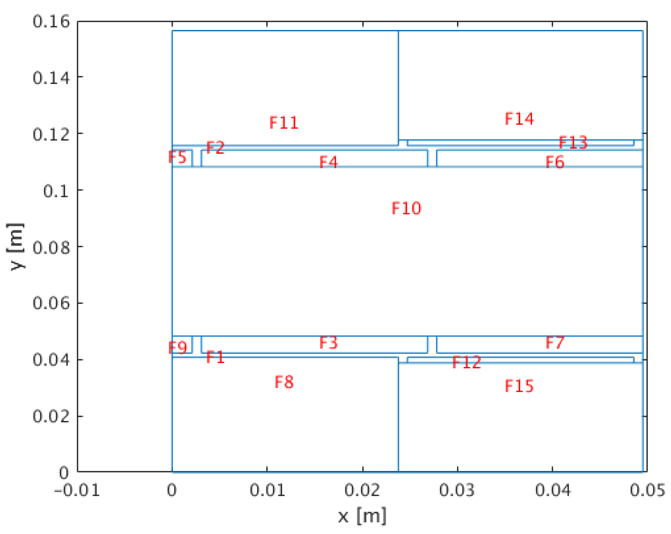
As mentioned before, due to the symmetry, all the calculations were done on the distance of 1/8 model of one machine phase. This fragment in the form of a 2D model, after importing to the MATLAB environment, was presented in Figure 4.
The areas of the numbers: 3, 4, 5, 6, 7 and 9 are permanent magnets lying on the rotor. The area number 10 represents a part of the rotor through which the magnetic field is closed within the area of one pole pitch. Areas 8 and 11 represent stator’s yoke, whereas areas 12 and 13 represent high magnetic permeability elements, serving as a magnetic shunt. Figure 5 presents distribution of the vector potential for rotor location that corresponds to the model presented in Figure 4, in the conditions of the occurrence of stator winding current flow of the value of and the magnetic field from permanent magnets.
Magnetic field distribution determined for one pole pitch of the modelled machine based on a 2D model is presented in Figure 6. Presented magnetic field distribution has been obtained based on a distribution of vector potential A presented in Figure 5 which was calculated using method discussed above, for a rotor position shown in Figure 4.
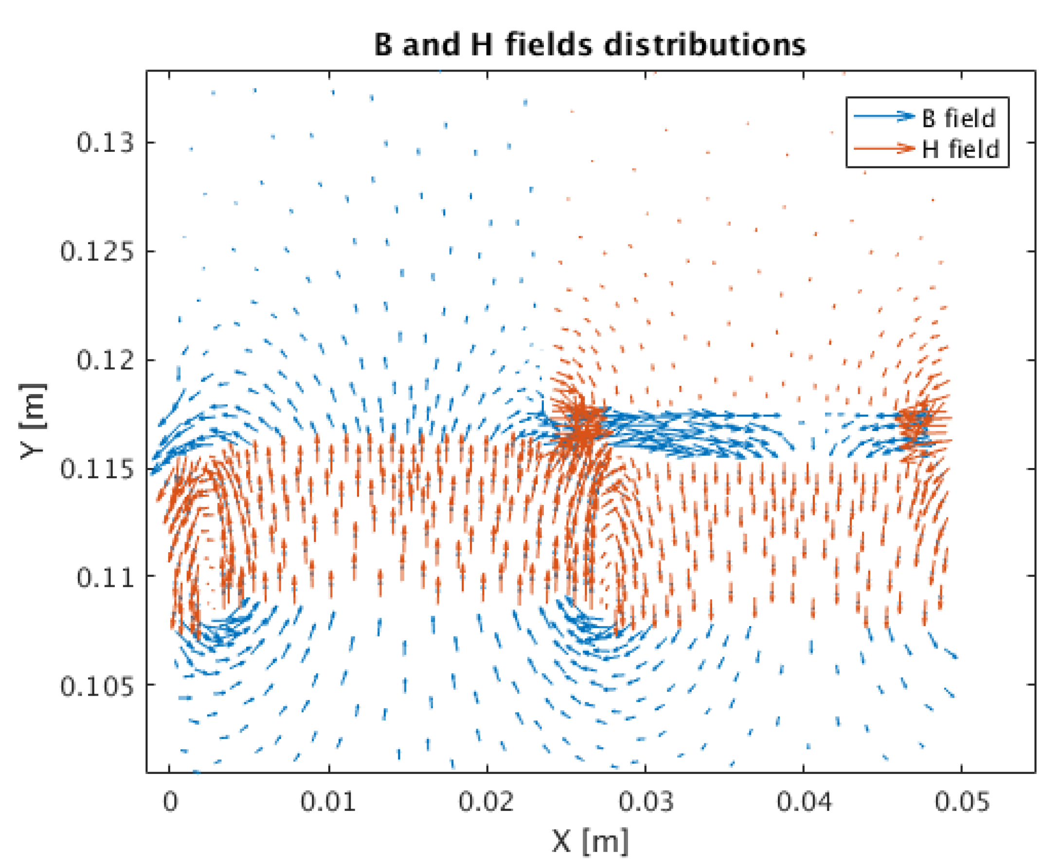
Figure 7 shows the resulting distributions of the magnetic field in close up, covering the upper part of the model. By analyzing Figure 7 it can be concluded that proposed 2D model allows correct reflection of the distribution of the magnetic field within the magnetic shunts and permanent magnets region.
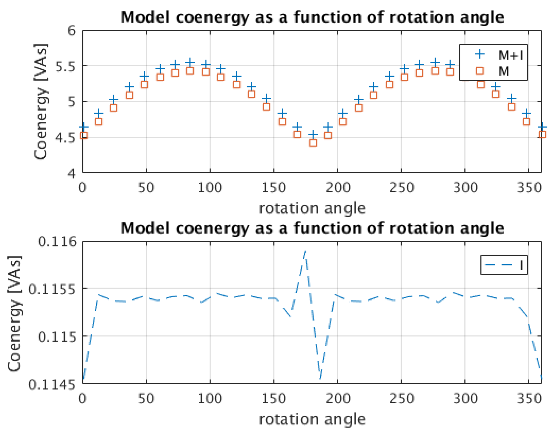
When analyzing Figure 5, Figure 6 and Figure 7 we may notice that vector potential distributions and magnetic field vectors are consistent with the adopted assumptions. This proves that the concepts of boundary conditions, which were presented in the previous sections, as well as the method of imposing them are correct. Figure 8 presents the results of magnetic co-energy calculations for the modelled machine, in the function of rotation angle, determined on the basis of 2D models of the single pole pitch of a machine with an angular step of . Those calculations were done with the proposed method, for the following situations:
- There is only magnetic field from permanent magnets
- Magnetic fields from permanent magnets and phase winding current are considered
- There occurs only magnetic field from phase winding current.
The upper part of Figure 8 presents the results of calculations of the magnetic co-energy value of the examined machine model as a function of the rotation angle, obtained using the proposed method. The values marked with red squares, described in the legend as ’M’, mean the co-energy values determined in the absence of current flow in the stator phase winding. Only the magnetic field from permanent magnets is taken into account. the values marked with a cross and described as ’I + M’ refer to the situation when the current flow of 20 A is also taken into account. The bottom part of Figure 8 presents the co-energy values determined for the case when the presence of the magnetic field from permanent magnets is not taken into account. The source of the field is only the phase winding current with a flow of 20 A.
Where current flow is understood as
- z—indicates the number of coil windings of phase winding
- —is the amperage of the current flowing through this winding.
6. Validation of Developed Method
To check the correctness of the obtained results, the full FEA has been conducted using Ansys/Maxwell software. The 3D analysis has been carried out for a fully symmetric part of presented model, with in this case is of a whole model. The analyzed part is presented in a Figure 9. After conducting several experiments, the discretization providing the magnetic field energy error at 0.1% has been chosen to apply for 3D computations.
In Figure 10. the magnetic field distribution over the radial cross-section of a model being tested is presented. By comparison, the field distribution presented in Figure 10 with the results of 2D computations presented in Figure 1 and Figure 7 it can be concluded that the magnetic field flow paths are reflected correctly in 2D model of exterminated machine. It can be concluded that in both cases the boundary conditions, as well as the directions of magnetization vectors, have been applied correctly for 2D analysis.
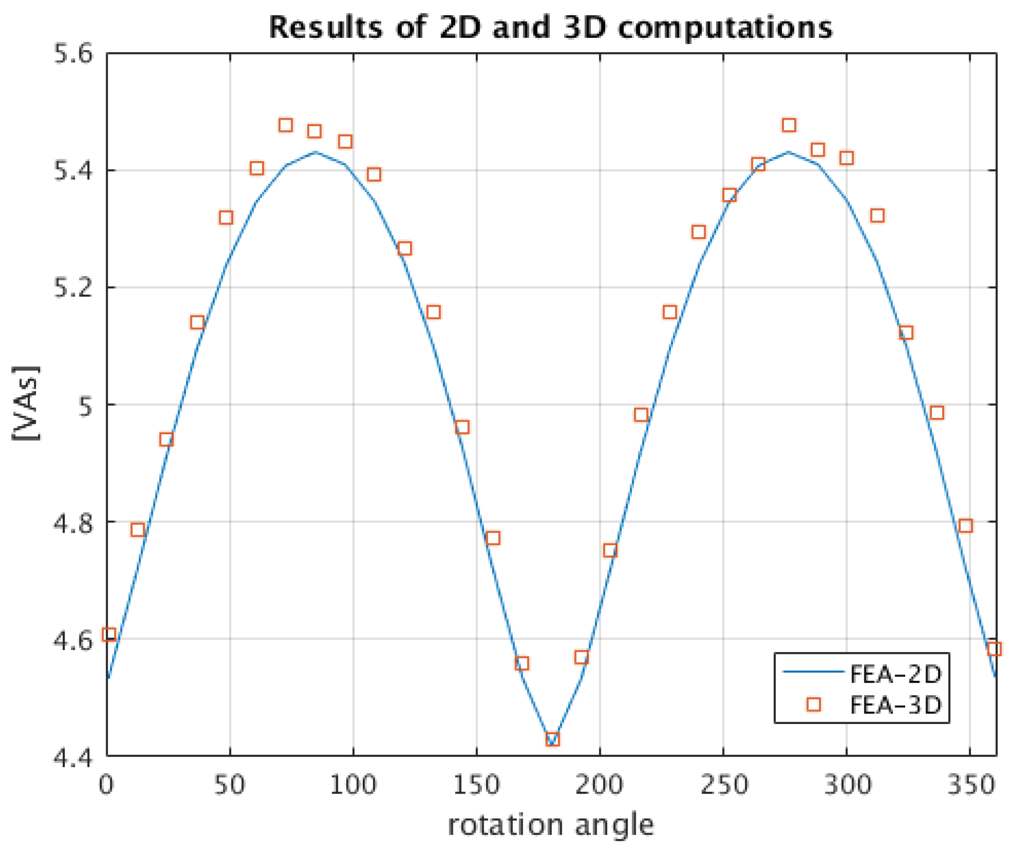
The co-energy values have been calculated based on 3D FEM using Ansys/Maxwell software, for three cases of considered magnetic field sources, as discussed in the previous chapter. Figure 11 presents a comparison of the results of the magnetic co-energy calculations of the tested machine, in the case of taking into account both the presence of a magnetic field from permanent magnets and the current flow in the stator phase winding.
Figure 12 presents the comparison between the results of co-energy, calculated in case when the phase current is assumed to be zero, based on 3D FEM and proposed method.
Figure 13 presents the comparison between results obtained for co-energy based on proposed method and 3D FEM, it concerns the case when only phase current is considered to be a source of magnetic field.
For the proper accuracy assessment, the relative norm of error between results of 3D FEA and these obtained by presented method, has been calculated as follows. The resulting values obtained for considered cases are presented in Table 1.
where:
- -indicates the resulting co-energy value obtained by 3D FEM for a certain angular position of rotor, denoted by index k
- -indicates the corresponding result obtained by proposed method.
If it comes to incorporation the proposed method into a numerical optimization procedure the consumption of computational time is crucial. It needs to be pointed out that to compute all the presented results less than 3 min is needed, while for presented accuracy calculations using 3D FEM takes more than 6 hours. Table 2 presents a juxtaposition of the number of elements in a model and a time consumption for both approaches being compared. The triangular elements with linear basis functions have been used in both 2D and 3D cases.
The obtained results show that proposed method provides a very good time to accuracy ration so it can be considered interesting if it comes to numerical optimization of TFM machines.
7. Conclusions
The purpose of the efforts was to develop a computationally efficient method for determining the magnetic co-energy as a function of rotational angle of transversal field permanent magnet (TFM) machine. The method of transforming TFM geometry into 2D system, with handle the influence of magnetic field that comes from stator winding phase coil current, have been proposed. The simplified 2D FE algorithm with model set in Cartesian coordinates was chosen to use. This approach has the advantage of being relatively easy to implement and use without any sophisticated software tools. Developed method has been validated by comparison with results of full 3D FEA. Obtained results allow a conclusion that due to its low time consumption, presented approach is well suited to incorporate in a numerical optimization procedure of TFM machines. The usefulness of the method developed and presented here is seen in the fact that not always, especially at the initial stage of design work, the designer has the possibility to perform a full FEM 3D analysis. In particular, in the case of numerical design optimization process, when such calculations would have to be carried out cyclically, the use of FEM 3D places great demands in terms of the amount of computing power needed and time. In this situation, the application of the approach described in this article would allow significant saving of time and the computing power needed to engage. In addition, these calculations can be carried out without the need for expensive dedicated software. It should be emphasized that the presented calculation method in the form presented here does not allow for taking into account the impact of phenomena associated with the saturation of the magnetic circuit. Experiments carried out in the Ansys/Maxwell environment show that this fact is not a problem for the structure analyzed in this work. This is due to the large size of the air gap, which causes the magnetic circuit to saturate to a negligible extent. Further work planned in this area will include: Further works on the method being developed, towards the possibility of testing other TFM machines known from the literature in which the influence of saturation of the magnetic circuit is significant. Development of modern methods of TFM machine control using the results of magnetic co-energy calculations.
Author Contributions
Conceptualization, L.G. and A.S.; methodology, L.G. and A.S.; software, A.S. and M.G.; validation, M.G. and D.M.; formal analysis, D.M.; investigation, L.G., A.S., M.G. and D.M.; writing—original draft preparation, A.S., L.G., M.G. and D.M.; writing—review and editing, S.A.; funding acquisition, D.M.
Funding
This project is financed by the Minister of Science and Higher Education of the Republic of Poland within the “Regional Initiative of Excellence” program for years 2019–2022; Project Number 027/RID/2018/19; the amount granted: 11,999,900 PLN.
Conflicts of Interest
The authors declare no conflict of interest.
References
- Kappatou, J.; Zalokostas, G.; Spyratos, D. 3-D FEM Analysis, Prototyping and Tests of an Axial Flux Permanent-Magnet Wind Generator. Energies 2017, 10, 1269. [Google Scholar] [CrossRef]
- Bang, D.; Polinder, H.; Shresthan, G.; Ferreira, J.A. Ring shaped transverse flux PM generator for large direct drive wind turbines. In Proceedings of the International Conference on Power Electronic and Drive Systems, Taipei, Taiwan, 2–5 November 2009; pp. 61–66. [Google Scholar]
- Svechkarenko, D.; Soulard, J.; Sadarangani, C. Parametric study of a transversal flux wind generator at no-load using three-dimensional finite element analysis. In Proceedings of the International Conference on Electrical Machines and Systems, Tokyo, Japan, 15–18 November 2009; pp. 1–6. [Google Scholar]
- Hasubek, B.E.; Nowicki, E.P. Design limitations of reduced magnet material passive rotor transverse flux motors investigate using 3D finite element analysis. In Proceedings of the IEEE Canadian Conference Electrical and Computer Engineering, Halifax, NS, Canada, 7–10 May 2000; pp. 365–369. [Google Scholar]
- Azarinfar, H.; Aghaebrahimi, M. Design Analysis and Fabrication of a Novel Transverse Flux Permanent Magnet Machine with Disk Rotor. Appl. Sci. 2017, 7, 860. [Google Scholar] [CrossRef]
- Zheng, P.; Zhao, Q.; Bai, J.; Yu, B.; Song, Z.; Shang, J. Analysis and Design of a Transverse-Flux Dual Rotor Machine for Power-Split Hybrid Electric Vehicle Applications. Energies 2013, 6, 6548–6568. [Google Scholar] [CrossRef]
- Wu, Y.; Kang, J.; Zhang, Y.; Jing, S.; Hu, D. Study of reliability and accelerated life test of electric drive system. In Proceedings of the IEEE 6th International Power Electronics and Motion Control Conference, Wuhan, China, 17–20 May 2009. [Google Scholar]
- Zhao, J.; Han, Q.; Dai, Y.; Hua, M. Study on the Electromagnetic Design and Analysis of Axial Flux Permanent Magnet Synchronous Motors for Electric Vehicles. Energies 2019, 12, 3451. [Google Scholar] [CrossRef]
- Peng, G.; Wei, J.; Shi, Y.; Shao, Z.; Jian, L. A Novel Transverse Flux Permanent Magnet Disk Wind Power Generator with H-Shaped Stator Cores. Energies 2018, 11, 810. [Google Scholar] [CrossRef]
- Zhu, S.; Zheng, P.; Yu, B.; Cheng, L.; Wang, W. Performance Analysis and Modeling of a Tubular Staggered-Tooth Transverse-Flux PM Linear Machine. Energies 2016, 9, 163. [Google Scholar] [CrossRef]
- Yang, X.; Kou, B.; Luo, J.; Zhou, Y.; Xing, F. Torque Characteristic Analysis of a Transverse Flux Motor Using a Combined-Type Stator Core. Appl. Sci. 2016, 6, 342. [Google Scholar] [CrossRef]
- Dobzhanskyi, O.; Mendrela, E.; Trznadlowski, A. Analysis of leakage flux losses in transverse flux PM synchronous generator. In Proceedings of the IEEE Green Technology Conference, Baton Rouge, LA, USA, 14–15 April 2011. [Google Scholar]
- Gieras, J.F. Transverse Flux Machine. U.S. Patent 7,830,057, 4 March 2010. [Google Scholar]
- Yu, B.; Zhang, S.; Yan, J.; Cheng, L.; Zheng, P. Thermal Analysis of a Novel Cylindrical Transverse-Flux Permanent-Magnet Linear Machine. Energies 2015, 8, 7874–7896. [Google Scholar] [CrossRef]
- Wang, W.; Zhou, S.; Mi, H.; Wen, Y.; Liu, H.; Zhang, G.; Guo, J. Sensitivity Analysis and Optimal Design of a Stator Coreless Axial Flux Permanent Magnet Synchronous Generator. Sustainability 2019, 11, 1414. [Google Scholar] [CrossRef]
- Wang, W.; Wang, W.; Mi, H.; Mao, L.; Zhang, G.; Liu, H.; Wen, Y. Study and Optimal Design of a Direct-Driven Stator Coreless Axial Flux Permanent Magnet Synchronous Generator with Improved Dynamic Performance. Energies 2018, 11, 3162. [Google Scholar] [CrossRef]
- Boldea, I.; Wang, C.X.; Yang, B.; Nasar, S.A. Analysis and design of flux reversal linear permanent magnet oscillating machine. In Proceedings of the 1998 Industry Applications Conference, 33th IAS Annual Meeting, St. Loius, MO, USA, 12–15 October 1998; pp. 136–143. [Google Scholar]
- Kou, B.Q.; Lou, J.; Yang, X.B.; Zhang, L. Modeling and analysis of novel transverse-flux flux reversal linear motor for long-stroke applications. IEEE Trans. Ind. Electron. 2016, 63, 6238–6248. [Google Scholar] [CrossRef]
- Wang, Q.; Zou, J.M.; Zou, J.B.; Zhao, M. Analysis and computer aided simulation of cogging force characteristic of a linear electromagnetic launcher with tubular transverse flux machine. IEEE Trans. Plasma Sci. 2011, 39, 157–161. [Google Scholar] [CrossRef]
- Dong, D.; Huang, W.; Bu, F.; Wang, Q.; Jiang, W.; Lin, X. Modeling and Static Analysis of Primary Consequent-Pole Tubular Transverse-Flux Flux-Reversal Linear Machines. Energies 2017, 10, 1479. [Google Scholar] [CrossRef]
- Hasanien, H.M.; bd-Rabou, A.S.; Sakr, S.M. Design optimization of transverse flux linear motor for weight reduction and performance improvement using response surface methodology and genetic algorithms. IEEE Trans. Energy Convers. 2010, 25, 598–605. [Google Scholar] [CrossRef]
- Marsden, J.E.; Tromba, A. Vector Calculus, 6th ed.; W.H. Freeman and Company: New York, NY, USA, 2012. [Google Scholar]
- Engwirda, D. Locally-Optimal Delaunay-Refinement and Optimisation-Based Mesh Generation. Ph.D. Thesis, School of Mathematics and Statistics, The University of Sydney, Sydney, Australia, 2014. Available online: http://hdl.handle.net/2123/13148 (accessed on 15 October 2019).
- Berhausen, S.; Paszek, S. Use of the finite element method for parameter estimation of the circuit model of a high power synchronous generator. Biul. Pol. Acad. Sci. Tech. Sci. 2015, 63, 575–582. [Google Scholar] [CrossRef]
- Vanoost, D.; Gersem, H.D.; Peuteman, J.; Gielen, G.; Pissort, D. Two Dimensional Magnetic Finite-Element Simulation for Devices With a Radial Symmetry. IEEE Trans. Magn. 2014, 50, 1–4. [Google Scholar] [CrossRef]
- Silvester, P.P.; Ferrari, R.L. Finite Elements for Electrical Engineers, 3rd ed.; Cambridge University Press: Cambridge, UK, 1996. [Google Scholar]
- Jin, J.M. The Finite Element Method in Electromagnetics, 3rd ed.; Wiley: Hoboken, NJ, USA, 2014. [Google Scholar]
- Sadiku, M.N.O. Numerical Techniques in Electromagnetics with MATLAB, 3rd ed.; CRC Press: Boca Raton, FL, USA, 2009. [Google Scholar]
- Li, J.; Chen, Y. Computational Partial Differential Equations Using Matlab; Springer: Berlin, Germany, 2010. [Google Scholar]
- Smoleń, A.; Gołębiowski, M. Computationally efficient method for determining the most important electrical parameters of Axial Field Permanent Magnet machine. BIuletin Yhe Pol. Acad. Sci. Tech. Sect. 2018, 66, 947–959. [Google Scholar]
Figure 1.
3D model of a TFM type machine—semi-view, semi-cross-section.

Figure 2.
The method of transforming TFM geometry into 2D a system, a semi-view, semi-cross-section of one pole pitch (on the left), view of the front with marked direction of development to the 2D system (on the right).
Figure 2.
The method of transforming TFM geometry into 2D a system, a semi-view, semi-cross-section of one pole pitch (on the left), view of the front with marked direction of development to the 2D system (on the right).

Figure 3.
Diagram presenting an obtained 2D model of one phase of the TFM machine, with a single pole pitch marked in a red box.
Figure 3.
Diagram presenting an obtained 2D model of one phase of the TFM machine, with a single pole pitch marked in a red box.

Figure 4.
The view of a 2D model of one pole pitch of the studied machine.

Figure 5.
vector potential distribution obtained for one pole pitch of the modelled machine, presented in Figure 4, in the conditions of occurrence of phase winding current and the magnetic field from permanent magnets.
Figure 5.
vector potential distribution obtained for one pole pitch of the modelled machine, presented in Figure 4, in the conditions of occurrence of phase winding current and the magnetic field from permanent magnets.

Figure 6.
Magnetic field distribution determined based on the presented 2D model for one pole pitch of the studied machine.
Figure 6.
Magnetic field distribution determined based on the presented 2D model for one pole pitch of the studied machine.

Figure 7.
Magnetic field distribution determined based on the presented 2D model for one pole pitch of the studied machine—close up covering the upper part of a model.
Figure 7.
Magnetic field distribution determined based on the presented 2D model for one pole pitch of the studied machine—close up covering the upper part of a model.

Figure 8.
Magnetic co-energy values as a function of rotation angle, determined using presented method. In case of considering the impact of both phase current and permanent magnets or only a magnets (up), considering only the phase current (down).
Figure 8.
Magnetic co-energy values as a function of rotation angle, determined using presented method. In case of considering the impact of both phase current and permanent magnets or only a magnets (up), considering only the phase current (down).

Figure 9.
Symmetrical section of one phase of the analyzed machine.

Figure 10.
The distribution of magnetic field over a radial cross-section of analyzed system.

Figure 11.
The values of co-energy determined for a machine being tested, based on 3D FEM (squares) and using proposed method (line). In case when both the permanent magnet and the phase current are considered to be a source of magnetic field.
Figure 11.
The values of co-energy determined for a machine being tested, based on 3D FEM (squares) and using proposed method (line). In case when both the permanent magnet and the phase current are considered to be a source of magnetic field.

Figure 12.
The values of co-energy determined for a machine being tested, based on 3D FEM (squares) and using proposed method (line). In case when no phase current is considered.
Figure 12.
The values of co-energy determined for a machine being tested, based on 3D FEM (squares) and using proposed method (line). In case when no phase current is considered.

Figure 13.
The values of co-energy determined for a machine being tested, based on 3D FEM (squares) and using proposed method (line). In case when only phase current is considered.
Figure 13.
The values of co-energy determined for a machine being tested, based on 3D FEM (squares) and using proposed method (line). In case when only phase current is considered.


Table 1.
Relative difference between values of co-energy calculated using 3D FEM and proposed method.
Table 1.
Relative difference between values of co-energy calculated using 3D FEM and proposed method.
| Case | Value of Error Norm |
|---|---|
| Both current and permanent magnets are included | 0.0091 |
| Only permanent magnets are included | 0.0099 |
| Only stator current is included | 0.0012 |
Table 2.
Model complexity and the time performance comparison.
| Parameter | 2D Calculations | 3D Calculations |
|---|---|---|
| Number of elements | 3753 | 230,000 |
| Total computational time | 2 min 32 sec | 6 h 24 min |
© 2019 by the authors. Licensee MDPI, Basel, Switzerland. This article is an open access article distributed under the terms and conditions of the Creative Commons Attribution (CC BY) license (http://creativecommons.org/licenses/by/4.0/).
Share and Cite
MDPI and ACS Style
Smoleń, A.; Gołębiowski, L.; Gołębiowski, M.; Mazur, D. Computationally Efficient Method of Co-Energy Calculation for Transverse Flux Machine Based on Poisson Equation in 2D. Energies 2019, 12, 4340. https://doi.org/10.3390/en12224340
AMA Style
Smoleń A, Gołębiowski L, Gołębiowski M, Mazur D. Computationally Efficient Method of Co-Energy Calculation for Transverse Flux Machine Based on Poisson Equation in 2D. Energies. 2019; 12(22):4340. https://doi.org/10.3390/en12224340
Chicago/Turabian StyleSmoleń, Andrzej, Lesław Gołębiowski, Marek Gołębiowski, and Damian Mazur. 2019. "Computationally Efficient Method of Co-Energy Calculation for Transverse Flux Machine Based on Poisson Equation in 2D" Energies 12, no. 22: 4340. https://doi.org/10.3390/en12224340
Note that from the first issue of 2016, this journal uses article numbers instead of page numbers. See further details here.