Flow Regime Analysis of the Pressure Build-Up during CO2 Injection in Saturated Porous Rock Formations


1
Department of Engineering, Oil and Gas Program, University of Nicosia, P.O. Box 24005, Nicosia 1700, Cyprus
2
Department of Civil Engineering and Geomatics, Cyprus University of Technology, P.O. Box 50329, Limassol 3603, Cyprus
*
Author to whom correspondence should be addressed.
Energies 2019, 12(15), 2972; https://doi.org/10.3390/en12152972
Submission received: 28 May 2019
/
Revised: 18 July 2019
/
Accepted: 24 July 2019
/
Published: 1 August 2019
(This article belongs to the Special Issue Computational Fluid Dynamics (CFD) 2018)
Abstract
:In this work, we are concerned with the theoretical and numerical analysis of the pressure build-up on the cap of an aquifer during CO2 injection in saturated porous rock formations in all flow regimes of the problem. The latter are specific regions of the parameter space of the plume flow, defined by the CO2-to-brine relative mobility and the buoyancy parameter (injection pressure to buoyancy pressure scale ratio). In addition to the known asymptotic self-similar solutions for low buoyancy, we introduce two novel ones for the high buoyancy regimes via power series solutions of asymptotic self-similarity equations. The explicit results for the peak value of pressure on the cap, which arises in the vicinity of the well, are derived and discussed for all flow regimes. The analytical results derived in this work are applied for the purpose of cap integrity considerations in six test cases of CO2 geological storage from the PCOR partnership, most of which correspond to high buoyancy conditions. The validity of the self-similar solutions (late time asymptotics) is verified with CFD numerical simulations performed with the software Ansys-Fluent. The result is that the self-similar solutions and the associated pressure estimations are valid in typical injection durations of interest, even for early times.
1. Introduction
It has been observed that the global temperature has increased over the years, causing adverse climatic effects. It is believed that one of the factors contributing to this global warming effect is the increasing demand in the combustion of fossil fuels to produce energy. Therefore, according to the International Energy Association, CO2 capture and storage (CCS) must be part of the strategy for mitigating climate changes by setting a target to control and decrease the global temperature at least by 2 °C until the year 2040. This target is by no means trivial to obtain, as it will require by the international community to invest 1.6 trillion dollars annually with most of this capital absorption to be in renewables, nuclear, and CCS. Regarding CCS projects, it has been estimated that 75 billion/year will be able to contribute to suppressing the global cumulative CO2 by as much as 13% by 2050. It is worth mentioning that related technologies for CCS are still under development and much focus is devoted from the oil and gas industry, because it presents similarities with enhanced oil recovery (EOR) and enhanced gas recovery (EGR). Currently, any CCS projects are economically viable primarily when they are combined with other oil and gas technologies like enhanced oil recovery (EOR) [1,2,3,4,5,6,7].
Suitable reservoirs for storing carbon dioxide are chosen as a function of depth because they should have thermodynamic conditions (pressure and temperature) that will ensure that the CO2 injected will remain thermodynamically stable and in supercritical state in order to guarantee efficient storage. Saline aquifers are considered promising for storing large quantities of carbon dioxide in the subsurface. Thermodynamically speaking, supercritical CO2 has a density much larger than gaseous CO2, and it is still small relative to the density of the resident brine, with a difference ranging from 250 kg/m3 to up to 950 kg/m3. This difference is attributed to formation depth, geothermal gradient, pressure gradient, surface temperature, and water salinity. Sequestration of CO2 in saline aquifers involves flow of both carbon dioxide and resident brine. The understanding of the multi-phase flows in porous media is of paramount importance to address various questions related to the CO2–brine multiphase flow properties such as the relative permeability and the viscosities of the brine and CO2, which in turn influence the injectivity of fluids in reservoir conditions [8,9], containment [10,11], pressure build-up [12,13], formation cap integrity [14,15,16], and long-term effectiveness [16,17].
The physical process of CO2 sequestration into the subsurface is usually described by a nearly immiscible multiphase flow of the supercritical CO2 and the resident fluid, for example, see the literature [18,19,20,21,22,23]. The difference in their densities leads to buoyancy effects mobilizing the carbon dioxide to reach the cap of the formation relatively fast, thus creating vertical gravity segregation between the CO2 (layering on the top) and the brine (recedes at the bottom) in the formation. Furthermore, according to the properties of these fluids, CO2 can migrate away from the injection site depending on its buoyancy and mobility relative to the brine. Usually, the modeling of this two-phase flow in porous media involves complete gravity segregation, that is, a sharp interface separates the two fluids. According to the Dupuit approximation, when the time scale required for buoyant segregation is small compared with the time scale required for horizontal propagation of this interface, then it can be assumed that the CO2 and the brine have reached pressure equilibrium in the vertical direction, so that the two fluids move only horizontally. A further assumption of negligible capillary pressure and negligible miscibility between the CO2 and the brine leads to the well-known non-linear diffusion equation that describes the dynamics of the sharp interface evolution [8,18,19,20,21].
Recently, researchers developed a flow regime analysis identifying the regime of validity of asymptotic solutions in the parameter space (λ, Γ) of this problem; λ is the CO2-to-brine relative mobility, and the buoyancy parameter Γ can be interpreted as the ratio of buoyancy to injection pressure scales, encoding the strength of buoyancy. Regimes I to III correspond to injection-driven flows with the injected fluid being highly viscous, equally viscous, and less viscous, respectively, than the resident fluid. For these regimes, simple analytical solutions exist. Regime IV is the buoyancy driven flow, for which we offer a novel analytical solution in terms power series. Finally, Regime V is the transition where the forces generated by fluid injection become comparable to the forces generated by buoyancy. This regime requires the numerical solution of the exact self-similar equation [9,21].
As a natural consequence of multiphase fluid flow in the aforementioned regimes from the work of [9,21], a pressure build-up will be created, and it has to be ensured that it will remain below the strength of the cap rock so as to ensure sure its safe fate over large periods of time. The caprock is an integral part of any sequestration project. The caprock, which is associated with the reservoir rock (CO2 storage target formation), has to be deep enough, it must be away from faults, and its mass must be dense and intact. The main petrophysical parameters of the caprock include uniaxial strength, young modulus, porosity, and permeability. A caprock should possess low permeability to keep the CO2 from seeping through it over a long period. The cap rock must also have high strength in both compression and tension, so as to be able to undertake the stress change during and after injection [15]. Even so, the above-stated properties of a good candidate caprock do not guarantee the avoidance of the following leakage-related risks involved in a CO2 sequestration project: (a) reactivation of faults, (b) induced shear failure of the caprock, (c) hydraulic fracturing (prior and during injection), (d) leakage through the injection well, and (e) capillary membrane seal pressure exceedance. Thus, these have to be studied in each project.
The caprock properties and CO2 interaction should be thoroughly studied with empirical, numerical, and analytical models for each project during planning and deployment of the CO2 injection process in order to reach closer to real case scenarios. Existing simplified analytical solutions for determining the maximum sustainable pressure often predict incorrect values, suggesting that the fully coupled problem (fluid flow mechanical deformation) must be considered. Nonetheless, the majority of CO2 injection simulations are only concerned with the multiphase flow problem without mechanical coupling [8,22,23,24]. These studies yield accurate results when reproducing small pilot CO2 injection projects. However, one may argue that the associated volumes of CO2 injected are small; therefore, caprock stability is not expected to yield visible results or be of concern. On the other hand, when considering the fully coupled problem, the computational burden is much higher than the hydraulic problem; therefore, significant loss of accuracy is expected while solving the fully coupled problem, especially when the deflection of the caprock is also important in the solution [25,26,27,28,29]. One possible reason for this high computational cost is that the mechanisms involved in the multiphase flow in porous medium coupled with the caprock are not yet fully understood. Clearly, there is still much work that needs to be done in terms of mathematical and numerical modeling in order to understand the involved mechanisms, and then in turn start improving both the accuracy and predictions to come closer to real case scenarios. In terms of physics, in addition to the propagation of the CO2 plume, it is important to understand the evolution of pressure, which may also include compressibility effects, because supercritical CO2 is highly compressible relative to the resident brine fluid. Analytical or semi-analytical works in this direction include those of [12,23,30].
In this work, we derive the cap pressure formulas in the flow regimes of the works of [9,21] and in particular at the location next to the well, that is, the peak of the cap pressure. Along the way, we provide an analytical solution for Regime IV in terms of power series, as well as the analytical solution of a region in the overlap of Regimes IV and V (which we call Regime IV+), together with the respective cap pressure expressions. Regime V, which by definition requires the solution of the self-similarity equation of the problem, is treated building on the work of our previous contribution [8], where we investigated in detail the self-similar plume interface evolution. In that work, a detailed comparative analysis was performed between the self-similar sharp-interface solution and the numerical simulation of a two-phase flow solver [31]. The non-linear self-similarity equation, first derived and discussed in the work of [32], is indeed susceptible only to numerical solution, but amounts to a far simpler and computationally economic than the one dealt with by the two-phase solver. Given that the self-similarity solutions are late time solutions, we set the derived cap pressure profiles against the results of a two-phase flow solver (which utilizes the volume of fluid (VOF) method suit of methods in CFD numerical calculations [31]). It is shown that the self-similar solutions are essentially correct as early as one buoyancy time-scale [8]. The whole machinery is then applied to cap integrity considerations, using the data of the works of [33,34,35] regarding two large geo-sequestration units in saline aquifers, the Lower Cretaceous sandstone formation in Newcastle and a limestone formation in the Madison group.
This work is organised as follows. In Section 2, we present the background theory of the self-similar plume evolution, the flow regime asymptotic solutions, and the associated pressure build-up analysis. In Section 3, we describe the numerical models that were created and solved with the CFD numerical solver [31]. In Section 4, we (i) present comparisons between the CFD numerical simulations and the solutions of the self-similar equation for the plume interface and pressure profiles across the aquifer, and (ii) apply the derived injection pressure results of Section 2 to caprock integrity for the two formations mentioned above. In Section 5, we present a summary of this work and certain conclusive remarks.
2. Theoretical Analysis
We model the spreading of the (supercritical) CO2 plume into a porous formation, initially saturated with brine, as an immiscible displacement problem obeying axisymmetry. The formation is assumed homogeneous and confined above and below by impermeable geological settings. It is also assumed that a sharp interface develops between the invading fluid (CO2) and the resident brine, which is immiscible, assuming vertical equilibrium and neglecting the capillary pressure. The fluids are taken to be Newtonian, incompressible, and chemically inert, as simplifying assumptions for the theoretical analysis.
The validity of the gravity segregation (sharp interface) and vertical equilibrium was discussed in the work of [36], based on that of [37]. Vertical equilibrium is maintained because of the large aspect ratio of the plume, that is, its radial extent is much larger than its thickness, at the mature stage of the plume evolution. In the case under consideration, the aspect ratio is roughly 100:1, leading to a negligible error of the order (1/100)2, according to the estimate of [36]. The assumption that the capillarity effects are negligible implies that the fluids are clearly segregated according to density. This assumption is less well founded, as capillary forces lead to a non-negligible transition saturation zone that may modify the sharp interface or invalidate this simplifying assumption [38,39,40,41]. Nonetheless, capillary effects are in general less important than the effects of gravity in this problem (see, for example, the work of [41]) and we shall neglect the capillary pressure effects.
The injected carbon dioxide propagates radially, eventually forming a continuous plume with a well-defined interface with the resident brine. The lower density and lower viscosity (i.e., higher mobility) of the CO2 relatively to the brine allow the injected carbon dioxide to move towards the top of the porous formation (Figure 1).
2.1. The Self-Similar Dynamics of the Plume Evolution
The equations governing the evolution of the CO2–brine interface have been developed in the works of [32] (see also the works of [36,42]). Let be the intrinsic permeability of the porous medium and is the porosity of the formation. The mass density of the CO2 will be denoted by and that of the brine by The dynamic viscosity of CO2 and brine will be denoted by and , respectively. The relative permeabilities associated with the two fluids are taken to be 1 for simplicity. We should note that in real applications, the relative permeabilities differ from the value assumed for this analysis (the maximum value of brine is 1, but for the CO2, it is rather near 0.6, as saturation cannot reach 100%). Let be the thickness of the CO2 plume at time and distance from the well. The time-dependence of all quantities will be left understood from here on. Q is the CO2 injection flow rate. The formation is bounded at the top and bottom by two impermeable layers at z = 0 (cap) and z = H (bed), as shown in Figure 1. Let p(r, z) be the pressure at distance r from the wellbore centre and z the depth from the cap. The assumption of vertical equilibrium explicitly reads
with the solution
The two branches are connected by continuity of pressure at the interface. We have introduced the following symbols the pressure function at the bed and cap: and , respectively.
Using the continuity of pressure at the interface to match the relations (2a) and (2b), we obtain
where the matching also produces the relation
From these relations, we obtain
Vertically averaging each of the relations 5a, 5b in the respective region, we also obtain
where the barred pressures are the vertically averaged values of the pressure in the indicated region. It is convenient here to introduce the mobilities of the CO2 and water, λc and λw, respectively, and the mobility ratio λ (relative mobility of CO2):
As discussed in the works of [8,32], the mobility ratio is one of the coordinates of the parameter space in this problem. The second is the gravity number Γ introduced below. The pressure gradients are related to the volumetric rates of each fluid, Qc and Qw, respectively, after integrating vertically the generalized Darcy law for the two-phase flow, as is usual when vertical hydrostatic equilibrium is assumed [32,43]. We obtain
Conservation of mass requires that Qc + Qw = Q (the well injection volumetric rate). Thus, we have
This equation relates the pressure (at the top of the aquifer) to the plume thickness h. The continuity equation, for example, for the brine, reads
Then, Equations (6b), (8b), and (9) allow us to re-write Equation (10) in the form
This equation has been studied in the works of [8,32,36]. One may define the buoyancy time scale as follows [8]:
where is the speed scale for the injected CO2 volume to traverse vertically the formation due to buoyancy and is the related time scale (buoyancy time scale). At times, larger than the buoyancy time scale one may look for self-similar asymptotic solutions. Thus, we define the dimensionless quantities by
and seek a solution of Equation (11) of the form , where is the normalized plume thickness and χ is the square of the self-similarity distance . We thus obtain the following self-similar equation:
where Γ is the buoyancy parameter [32]:
2.2. Pressure Analysis in the Flow Regimes of Plume Evolution
A detailed comparison between the solutions of exact self-similar equation, Equation (14), and numerical simulations, was performed in the work of [8] at the level of CO2 plume–brine interface and its evolution. Here, we are interested in extending the comparison of pressure profiles, also studying the early time behaviour of the self-similar solutions, and eventually using the resulting equations for cap integrity considerations. Hence, we explicitly derive equations for the pressure profiles along the aquifer, specializing these equations for the various flow regimes of the problem, as classified below.
Using the dimensionless distance and plume thickness defined through the relations in Equation (13), Equations (5) and (9) give
which integrates to
We have introduced the locations where the plume–brine interface meets the bed and the cap of the aquifer, and , which, in dimensionless form, read and , respectively. These correspond to the leading and trailing edges of the plume, respectively. Also, in accordance with our definition, in terms of the self-similarity coordinate, we have and . Given a solution or , the cap pressure profile can be calculated.
Most of our considerations will be based on Equation (17). One should bear in mind that r < rcap and hence Equation (17) express the cap pressure at location r relative to the cap pressure at the tip of the plume. The first term in the brackets of Equation (17) corresponds to pressure build-up at the cap due to injection; the second term corresponds to pressure build-up due to buoyancy. At the same time, buoyancy decreases the thickness x of the CO2 plume. Hence, buoyancy also enhances the pressure build-up due to injection, at least for CO2 relative mobility λ greater than 1.
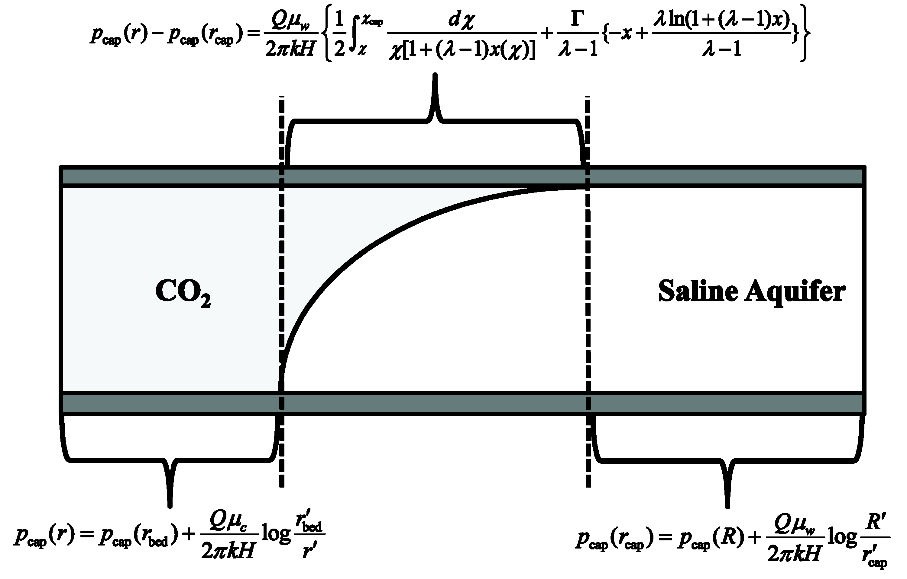
The cap pressure at the end of the interface pcap(rcap) is fixed by the boundary conditions for the pressure at large distances. In the numerical simulations, this amounts to pure hydrostatic brine pressure at some large distance R. In general, there will be three regions, as seen in Figure 2: the inner (pure CO2) region; the two-phase, that is interface region; and the outer (pure brine) region. Applying Darcy’s law in the outer region, we have
where the boundary condition implies that we should set pcap(R) = 0. Then, in the interface region, Equation (17) holds. In the inner region, Darcy’s law gives
where pcap(rbed) is provided by Equation (17). Thus, one obtains the cap pressure profile throughout the formation. Figure 2 shows the different regions of the pressure and their matching to obtain the total pressure profile.
For cap integrity considerations, we are interested in the cap pressure at the well relative to the cap pressure at the tip of the plume: P = pcap(rw)−pcap(rcap). We shall label P as the injection pressure. There are two cases. First, the trailing edge of the plume lies away from the well. Then, P can be written as
In the above, we introduced the pressure scale P0, through which we will express the pressure in dimensionless form:
The pressure build-up given in Equation (19) consists of three components:
Second, there is no trailing edge of the plume; the plume does not cover the entire length of the well. This happens for high buoyancy solutions where the idealized modeling of the interface predicts that there is no pure CO2 region near the wellbore up to a certain height [8,9,21]. Then, P reads
Whether Equation (19) or Equation (22) applies depends on the mobility and buoyancy parameters, that is, the regime of the parameter space of the flow. The flow regimes of the problem with regard to the asymptotic solubility of the self-similarity Equation (14) have been discussed in the works of [9,21,43], shown on the parameter space in Figure 3. Below, we summarize these findings, in our notation, also calculating the injection pressure in each case. In the previous formulas, we introduced the self-similarity coordinate χw and radial distance rw of the well:
One should bear in mind that these quantities depend explicitly on time and are directly known by the given parameters of the problem.
Regime I: Γ<<1 and λ< 1 (low buoyancy, low CO2 mobility).
The injection pressure P from Equation (19) for this regime explicitly reads
Regime II: Γ<<1 and λ= 1 (low buoyancy, unit CO2 mobility).
From Equation (19), the injection pressure here reads
Regime III: Γ<<1 and λ>1 (low buoyancy, high CO2 mobility).
From Equation (19), the injection pressure for this regime reads
Regime IV: Γ >> 1 (high buoyancy). This region of the parameter space is specified as shown in Figure 3. Roughly speaking, one may say that it corresponds to cases where Γλ and Γ/λ are bounded from below by order 1 constants, for large and small λ, respectively.
For this regime, no analytical solution is known. We present here a solution in terms of power series. The self-similarity Equation (14) in the large buoyancy limit takes the form [21,43]:
where
with the boundary conditions . Also, one may show that
It is straightforward to show that the solution of Equation (27) can be expressed as a power series with respect to the tip of the plume,
where the coefficients are generated by the recursive relation,
Equation (30) implies that all are positive. For large values of the index i, one may verify numerically that (roughly) , which suggests that the series is convergent for 0 < y < 1. The convergence of the series in the neighborhood of y = 0, that is near the well, is painfully slow, nonetheless the relation in Equation 31 allows the quick generation of thousands of terms. For example, one easily finds that I = 0.179. The asymptotic behavior near y = 0 can be derived as follows. Integrating Equation (27) from y to 1, we obtain
utilizing also the boundary conditions at y = 1. Upon further integrating, it is easy to see that
for y~0. The functional form of this solution has been anticipated by the authors of [36]. The asymptotic behavior given by Equation (33) can be used as a test of accuracy of the series given by Equations (30) and (31) in the neighborhood of y = 0.
Given that in the generic case of Regime IV, there is not trailing edge of the plume, the injection pressure P will be calculated by Equation (23). By Equations (28) and (29),
where f is given by Equations (30) and (31). The thickness of the plume at the well is
A closed form expression of the injection pressure in this regime is not possible, but we may easily derive an asymptotic expression for very large buoyancy. Indeed, Equations (29), (33), and (34) tell us that for large λΓ, the CO2 plume will form a very long but very thin layer, that is, x and xw are small. Then, it is straightforward to show that Equation (22) simplifies to
where the tilde indicates the fact that this result is asymptotic for large λΓ. We also used Equation (35).
In the limit of large λΓ, we may approximate f by its asymptotic given by Equation (33), because the argument of the function f in Equation (36) is necessarily very small. Using Equations (29) and (33), we finally find
Regime V: Intermediate buoyancy. It is shown in Figure 3. It corresponds to the cases where a numerical solution of the self-similarity Equation (14) is necessary. Injection pressure may be calculated by Equations (19) or (22), depending on the conditions of the problem.
Regime IV+: The solution presented for Regime IV can be modified to hold well on a region on the overlap of Regime IV and Regime V, as given in Figure 3. Put differently, one may find a solution for regime V near its boundary with Regime IV. This solution will be discussed in detail in a separate publication, but the argument leading to it is as follows.
The derivation of Equation (27) follows from the approximations that x << 1 and (λ−1)x << 1 for the most part of the plume [21,43]. The approximation x << 1 follows for the fact that for large buoyancy (Γ >> 1), the plume forms a thin layer near the cap. Now, the analysis of the works of [21,43] encoded in Equation (28) implies that x scales as
Then, the approximation (λ–1)x << 1 implies (roughly) that Γ >> λ, which is encoded in the boundary curve Γ = 4λ between Regimes IV and V, according to the discussion of the authors of [21,43]. Consider now a large buoyancy approximation (Γ >> 1), which means that x << 1 will be assumed, but consider also a large mobility approximation, such that (λ−1)x >> 1. Then, the self-similarity Equation (14) takes the form
This equation is similar to the one leading to Equation (27), which defines the solution of Regime IV [21,43] with the following modifications:
and the additional term (λx)-1 in the square brackets. One may then seek for solutions that are defined by equations similar to Equations (28) and (29) under the substitution in Equation (40). The dimensionless plume thickness x for such a solution scales as follows:
and hence, the additional term (λx)−1 scales as
given that we have assumed large mobility. This term can be dropped in Equation (39) if
Then, the remaining equation can be given exactly in the form of Equation (27), given Equations (28) and (29), under the substitution in Equation (40). In all situations, the solution of Regime IV+ is exactly given by the asymptotic solution of Regime IV under the substitution in Equation (40). It is expected to hold well for large buoyancy and mobility as long as Equation (43) holds. Boundary curves for this regime, analogous to the ones shown in Figure 3, involve systematic comparison with the numerical solutions of exact self-similar Equation (14), and will be given in a separate publication.
3. Numerical Modeling
As explained in Section 2, owing to the inherent nonlinearities in the multiphase flow regimes, the immiscible displacement of CO2 displacing brine possesses special challenges in the modeling because of the interaction of the fluids with the porous formation. Closed form analytical solutions are rare and apply under specialized or ideal conditions, which is thus computational modeling proof to provide valuable tools for investigating the dynamics of the CO2 front invading the porous medium and the associated pressure build-up. The numerical computations were carried out in Ansys-Fluent, a nonlinear CFD code [31].
The volume of fluid (VOF) method is a widely used scheme for moving boundary problems [8,31]. The moving interface with this method can be represented explicitly on a fixed cell grid and the tracking is achieved by changes in the volume of each fluid in the grid cells. Those grid cells that the volume fraction of either fluid differs from (0) or (1) correspond to the interface. This way, the interface and its evolution is a natural outcome of the solution algorithm. Furthermore, another important property of the VOF method is that it conserves exactly the volume of the fluids in each cell. Another important feature of the VOF method is that if a disruption in the interface is observed, it presents the capability to reconnect as part of the computational solution. This formation of the moving boundary is very elegant in CFD modeling of the CO2 sequestration problem [8,31].
The governing equations of multiphase flow are solved with finite volumes. The volume fraction for each fluid phase satisfies mass and momentum conservation. The latter includes a gravity term inducing segregation of the phases and a sink term that incorporates Darcy’s law in order to model the porous medium [8,31].
The PISO (pressure implicit with splitting of operators) method was used for the approximation of the pressure in the multiphase flow. This method is especially useful in nonlinear and unsteady flow problems. Some positive aspects of the PISO are that no under-relaxation is applied and the momentum corrector step is performed more than once. The algorithm can be described with the following steps: (1) set the boundary conditions, (2) solve the momentum equations for the intermediate velocity field, (3) calculate the mass fluxes at the cells, (4) compute the pressure, (5) correct the mass fluxes, (6) correct the velocities with the new pressure values, (7) update the boundary conditions (if necessary), (8) iterate from (3) for a prescribed number of times, (9) increase time step and continue from step (1). Steps (4) and (5) are repeated for a prescribed number of times to correct for non-orthogonality of the control volumes in the numerical solution [8,31].
The considered domain was discretized to 5000 m × 30 m so as to ensure vertical equilibrium, for the gravity segregation assumption to hold [36,37]. The wellbore location is at the left corner (Figure 1). The wellbore radius is set to rw = 0.15 m. Given the large horizontal dimensions of the formation, the size of the wellbore radius becomes negligible and its effects can be ignored. The model is axisymmetric in agreement with the theoretical model of Section 2. The injection of the CO2 performed at the wellbore constitutes the inlet boundary condition. To simulate the impermeable rock layers above and below the aquifer, no flow wall boundary conditions were considered at these locations. Finally, the outlet boundary condition of zero-gauge pressure was imposed in order to ensure flow towards the outer boundary of the models. A sufficient fine mesh around the wellbore and in the vicinity of the caprock was used, so as to effectively track the fine changes at the interface of the two fluids and to resolve numerical instabilities arising around the interface, which results in pressure changes in the various flow regimes of the problem.
In our previous contribution [8], we analysed in detail the mesh dependency of the problem in an attempt to avoid uncontrolled generation of grid cells, as well as to save computational time. In that work, we used biased mesh and created four same models with 3 k, 12 k, 48 k, and 192 k to solve the same problem, which has shown that, balancing the solution accuracy with efficient computational time, the 48 k grid cells are the optimum. The results presented in this work correspond to simulations of 48 k grid cells. The grid spacing in the radial direction starts with a spacing of 0.96 m and increases geometrically by a factor of 1.0038. Totally, there were 800 grid cells in those directions. The grid spacing in the vertical direction starts with a spacing of 0.145 m at the cap and increases geometrically with a factor of 1.0364. Totally, this includes 60 grid cells in the vertical direction. Roughly one-third of the mesh is used near the cap in order to capture fine physical changes in the interface evolution and the associated pressure build-up. The calculations were carried out in Ansys-Fluent, a nonlinear CFD code suit of programs [31]. The usual eight-node tetrahedral cell elements were used to model the fluid flow in the aquifer and the interface evolution process. The computation of the fluid diffusion in the porous domain and the interface evolution process with the associated pressure build-up is performed by the displacement of the dense fluid (brine) by the less dense (CO2) in the cells center.
4. Results and Discussion
In this section, we present the results from the multiphase flow analysis performed for the modeling of the CO2 plume evolution and the respective pressure build-up into a porous formation. In our previous work [8], we investigated the following cases that cover a practically interesting region of the parameter space (Γ, λ). These values are shown in Table 1. The brine and CO2 data are taken from the work of [22]. Such values cover a range of cases that exhibit qualitative distinct and interesting behavior. The input parameters used for the numerical computations given in Table 1 include the dimensions of the wellbore and the formation, the porous rock and fluid properties, as well as the pumping parameters.
In the analysis to follow, we show the influence on the interface evolution and the respective pressure build-up, for mobility ratios corresponding to low and high mobility, and for fast injection (low buoyancy) to slow injection (high buoyancy).
4.1. Comparison of Computational Results with the Solution of the Self-Similar Equation for the Interface
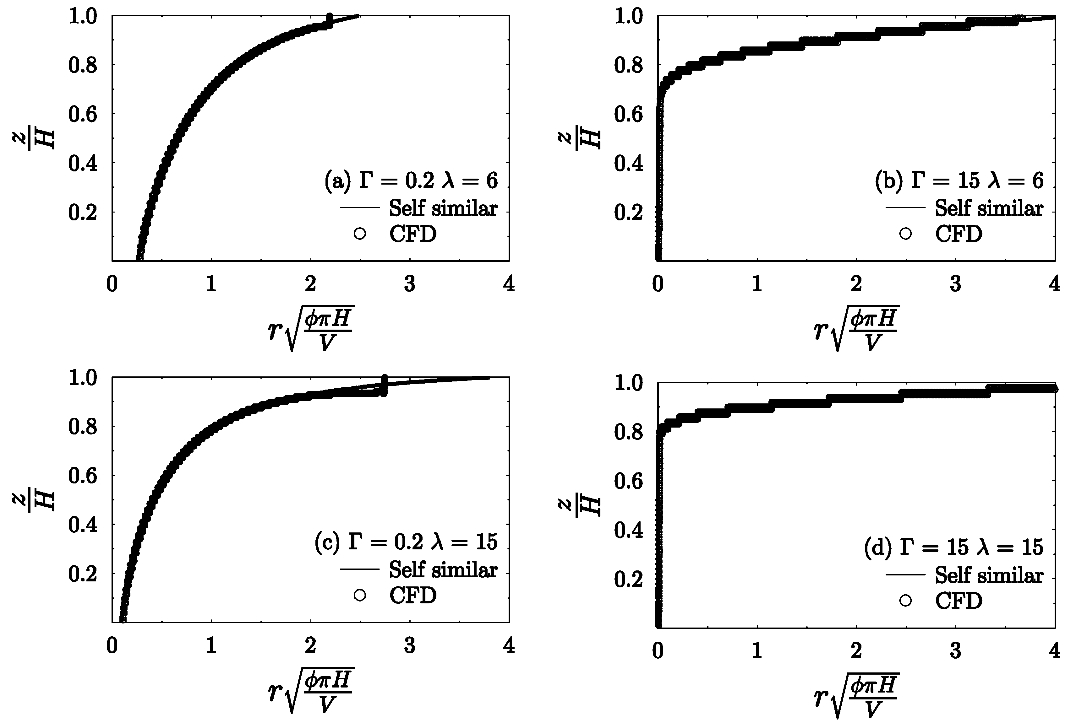
In this section, we compare the results of the full numerical solutions with the numerical solutions of the self-similar Equation (14), as discussed in the work of [8]. Figure 4 presents this comparison for the cases of fast (Γ = 0.2) and slow (Γ = 15) injection for mobilities λ = 6 and λ = 15. All results presented illustrate the interface at the mature state of evolution. For the choice of parameters of Table 1, the buoyancy time-scale defining the maturity of the interface evolution, given by Equation (12), is 2.2 years. For all cases, we observe that the full numerical solution and the solution of the self-similar Equation (14) are in excellent agreement. As expected on general theoretical grounds (Section 2), the high buoyancy cases cause the CO2 to accumulate from the early stages near the cap and extend to large distances in the porous formation, creating a relatively thin and long plume. This effect is enhanced by higher CO2 relative mobility λ. On the other hand, in fast injection scenarios, the plume covers the whole length of the well advancing, so that the leading and the trailing edges of the plume are much closer to each other than the slow injection scenarios. This means that the plume does not extend to large self-similar distances in the formation. Of course, the higher mobility causes the plume to extend further compared with the lower mobility case. The small discrepancy observed is explained as follows. The (high mobility) CO2 advances faster than it can diffuse, hence the trailing edge of the plume shows a tendency to slow down. The diffusion relaxation time should be larger than the buoyancy time scale τbuoyancy (given in Equation (14)) by a factor of the order of the aspect ratio of the CO2 plume. Indeed, the full numerical simulations show that the phenomenon diminishes slowly with time.
4.2. Comparison of Computational Results with the Solution of the Self-Similar Equation for the Pressure
This section is devoted to the comparison between the pressure profiles across the formation for various times, between the computationally obtained results and the solutions of the self-similar equation, as discussed in Section 2, applying the pressure Equations (17)–(19). In Figure 5, the vertical axis is the dimensionless pressure, while the horizontal axis is the self-similarity radial distance. The cases correspond once more to the fast and slow injection, Γ = 0.2 and Γ = 15, respectively, and for mobility, λ = 6 and λ = 15, respectively. The curves in each figure correspond to different times scaled by the buoyancy time: the top curve corresponds to t = 1.0τ, while every lower curve refers to a later time by 1.0τ. As just mentioned, the higher pressure profile arises in the earliest time considered, while as time progresses, the pressure is reduced by being diffused in larger distances in the formation. Also, the peak value of the pressure profile for all times is observed in the vicinity of the well, thereby suggesting high integrity risk near wellbore, as will be discussed later. We observe that the fast injection and lower mobility scenario (Figure 5a) induced higher peak pressures (pressure at the well) than the higher mobility case (Figure 5b). As expected, slow injection induces lower peak pressures by nearly two orders of magnitude, especially when the CO2 mobility is higher (Figure 5c,d). One should also observe that the agreement between the pressure profiles of the numerical solutions and the self-similarity solutions exhibits impressive agreement even at such early times as t = 1.0τ. This is practically very important, as it implies that the self-similarity equation can be applied, for example, for integrity estimations, at much earlier times than what one could expect. The exception seems to be the fast injection and high mobility scenario, where it requires at least 4.0τ for deviations from the numerical solution to become insignificant. That could be possibly attributed to the incomplete self-similarity phenomenon discussed for this case above (Section 4.2). One should observe that the pressure may become comparable to the rock tensile strength (Figure 5a,b) if the rate of CO2 injected is large. Of course, this may also be the case for the slow injection conditions (Figure 5c,d) for a different set of geologic and hydraulic parameters.
4.3. Pressure Build-Up Analysis for Cap Integrity Considerations
The following analysis is concerned with the application of the results of Section 2.2 in the case studies of the work of [33]. These cases include two geo-sequestration sites, which are two large saline aquifers: The Lower Cretaceous (sandstone) formations and the Madison Group (limestone) formations. The Lower Cretaceous formations include a lower aquifer unit and an upper aquifer unit, which are sandstones separated by a competent shale aquitard (Cretaceous A, B, C). The Madison unit is a group composed solely by three carbonate formations (Madison A, B, C). The geologic and hydraulic properties can be found in the work of [33].
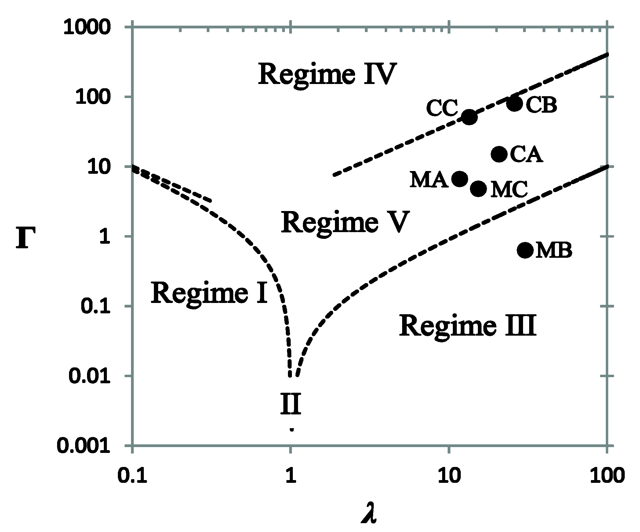
We first identify the flow regimes on the (λ, Γ) parameter space of each of the six cases, following our discussion in Section 2.2. The results for the mobility and buoyancy parameters and the corresponding flow regimes are given in Table 2 and presented pictorially in Figure 6: Madison B maps in flow Regime III; Madison A, C and Cretaceous A fall into Regime V; while Cretaceous B and C fall on what we have called Regime IV+.
According to the discussion of Section 2.2, these results imply that the pressure analysis should be based on the solutions of the exact self-similar equation for the cases of Madison A, C and Cretaceous A. These cases form an interesting set of examples where the analytical asymptotic solutions do not apply. They follow from the injection pressure formula (Equation (22)) using the numerical solution of the exact self-similar Equation (14). The cases of Cretaceous B and C can be treated using the novel asymptotic solution of Regime IV+ presented in this work. The results for the injection pressure, that is, the cap pressure next to the well, are shown in Table 2. The calculations are done using the numerical solutions of Equation (14) and applying Equation (22) or Equation (19). Also, where applicable, the respective analytical solutions are applied. The time horizon used in these calculations is 50 years. The results are also shown in Figure 7 in terms of the dimensionless pressure against the buoyancy parameter Γ.
In Table 2, we also include the results for the injection pressure formula given in the work of [33] and derived in the work of [12] under the assumptions that (i) buoyancy is negligible; (ii) the plume, the brine, and formation are compressible (with constant compressibility coefficients); and (iii) the inertia of the moving plume is taken into account by including a (Forchheimer) quadratic term in the Darcy law. In our notations, this reads as follows:
where γ = 0.5772 is the Euler–Masceroni constant. and are the compressibilities of the brine and the formation, respectively. The constant b is the Forchheimer inertial parameter [12]. The other quantities were defined in Section 2. Our results cannot be directly compared with the results of [33], because the two analyses are not based on completely the same physics (our analysis covers high buoyancy effects, while those of [12,33] consider compressibility and inertial effects). Nonetheless, a few interesting comments may be made in light of what we have learned in Section 2.2.
One may observe that the first terms in Equation (44), which read
can be recognized as the single-phase Darcy pressure build-up in the CO2 rich region and the injection pressure build-up, by comparing with Equation (26b) of the flow regime III in Section 2.2. As expected, the buoyancy pressure build-up term of Equation (26b) (the term proportional to the parameter Γ) is missing in Equation (44). The rest of the terms in Equation (44) clearly represent the compressibility and inertial effects, although the compressibility terms do not have a smooth limit to the no compressibility case.
Figure 6 shows that—with the exception of Madison B—the conditions of all formations correspond to high buoyancy, rendering Equation (44) virtually inapplicable for these cases. It may then be no surprise that, as can be seen in Table 2, the injection pressure for the high buoyancy cases of the Cretaceous A, B, and C formations is consistently higher when calculated through the self-similar solutions (and Equation (22)) than via Equation (44). This occurs in spite of the different mobility from case to case, and the inclusion of the compressibility and inertial effects in Equation (44). This finding is also shown in Figure 7, through the indicated curves, in terms of the injection pressure scaled by P0 (defined in Equation (20)) as a function of the buoyancy parameter Γ. This implies that the high buoyancy effects are not negligible compared with the compressibility of inertial effects, as far as those effects are described by the respective components of Equation (44).
Finally, Figure 7 includes the results of the application of the analytical solutions given in Section 2.2 in the three cases in which they are applicable. The results are also given in Table 2. The outcomes of the analytical solutions are shown in red crosses. We see that the Regime IV+ cases, which happen to be the highest buoyancy ones, reproduce quite well the results of the numerical solutions of the exact self-similar equation (Equation (14)). On the other hand, the analytical solution of the low buoyancy case (Regime III) deviates significantly from the results of the self-similar equation. The main reason is that the low buoyancy asymptotic solution actually corresponds to negligible buoyancy and is decently accurate only for Γ much smaller than 1.
5. Summary and Conclusions
In this work, we performed an analysis regarding the pressure build-up in the flow regimes arising in the CO2 injection problem in saturated porous rock formations. The purpose of this analysis emanates from the need to quantify the pressure exerting at the cap rock during CO2 sequestration. For this reason, we derived expressions for the pressure during injection and applied them to saline aquifers for cap rock integrity considerations. The pressure expressions derived in this work were applied by calculating estimates for the injection pressure for six aquifer test cases belonging to two different formations of geological importance (sandstone and limestone formations) considered excellent CO2 sequestration sites.
The flow regimes of the problem allow the derivation of analytical results for the pressure, valid in specific regions of the parameter space of the plume flow, defined by the CO2-to-brine relative mobility and the buoyancy parameter (injection pressure to buoyancy pressure scale ratio). In addition to the known asymptotic solutions of Regimes I, II, and III, we introduced two novel analytical solutions, one applying to Regime IV and the second to an overlap between Regime IV and V, which we named Regime IV+. These latter regimes correspond to high buoyancy and mobility conditions and they are rather important in practice. We showed that three of these test cases map into Regime V, where the numerical solution of the exact self-similar equation (Equation (14)) finds excellent application. Furthermore, two other test cases map into Regime IV+ and the associated analytical solution was utilized for the pressure estimation in the formation.
The main contributions of our analysis can be outlined as follows: (A) We provided the pressure build-up relations for all flow regimes (I–V) in the CO2 injection problem in saturated porous rock formations. (B) We provided explicit analytical solutions for regimes IV and IV+. (C) An important matter is the applicability of the self-similarity equation and its flow regime asymptotic solutions. Self-similar solutions are expected to apply to late times, but we showed, through CFD numerical simulations utilizing a two-phase flow solver, that self-similar solutions are essentially applicable as early as one buoyancy time scale. In most of the test cases considered, the buoyancy time scale is about 10 years or less, which makes the self-similar solutions applicable for design durations of several decades. (D) Both the self-similar and CFD models are capable of providing excellent estimates for the pressure build-up for a wide range of buoyancy parameters and fluid mobilities.
The outcome of our analysis in the direction of cap integrity considerations is that injection pressure estimates in high buoyancy conditions, that is, relatively slow injection, require application of the pertinent asymptotic solutions, or the direct numerical solution of the self-similarity equation. One should bear in mind that application of unsuitable asymptotic results leads to significant under-estimation of the injection pressure, which may produce erroneous estimates. Another approach is to utilize CFD solvers for the full analysis.
Future work on this subject will involve the fluid and formation compressibility effects, as well as the inertial effects of the plume. Undoubtedly, such considerations can be extended through asymptotic analysis in the high buoyancy regimes as well.
Author Contributions
Both authors contributed substantially to the work reported.
Funding
This research received no external funding.
Conflicts of Interest
The authors declare no conflicts of interest.
References
- International Energy Association. Climate Change; IEA: Paris, France, 2015. [Google Scholar]
- European Commission. Directive 2009/31/EC of the European Parliament and of the Council of 23 April 2009 on the geological storage of carbon dioxide and amending Council Directive 85/337/EEC, European Parliament and Council Directives 2000/60/EC, 2001/80/EC, 2004/35/EC, 2006/12/EC, 2008/1/EC and Regulation (EC) No. 1013/2006. Off. J. EU 2009, 5, 114–145. [Google Scholar]
- Metz, B.; Davidson, O.; de Coninck, H.; Loos, M.; Meyer, L. (Eds.) IPCC Special Report on Carbon Dioxide Capture and Storage; Cambridge University Press: Cambridge, UK, 2005. [Google Scholar]
- Papanastasiou, P.; Papamichos, E.; Atkinson, C. On the risk of hydraulic fracturing in CO2 geological storage. Int. J. Numer. Anal. Method. Geomech. 2016, 40, 1472–1484. [Google Scholar] [CrossRef]
- Blunt, M.; Fayers, F.J.; Orr, F.M., Jr. Carbon dioxide in enhanced oil recovery. Energy Convers. Manag. 1993, 34, 1197–1204. [Google Scholar] [CrossRef]
- Adu, E.; Zhang, Y.; Liu, D. Current situation of carbon dioxide capture, storage, and enhanced oil recovery in the oil and gas industry. Can. J. Chem. Eng. 2019, 97, 1048–1076. [Google Scholar] [CrossRef]
- Ravagnani, A.G.; Ligero, E.L.; Suslick, S.B. CO2 sequestration through enhanced oil recovery in a mature oil field. J. Pet. Sci. Eng. 2009, 65, 129–138. [Google Scholar] [CrossRef]
- Sarris, E.; Gravanis, E.; Papanastasiou, P. Investigation of self-similar interface evolution in carbon dioxide sequestration in saline aquifers. Transp. Porous Media 2014, 103, 341–359. [Google Scholar]
- Guo, B.; Zheng, Z.; Bandilla, K.W.; Celia, M.A.; Stone, H.A. Flow regime analysis for geologic CO2 sequestration and other subsurface fluid injections. Int. J. Greenh. Gas Control. 2016, 53, 284–291. [Google Scholar] [CrossRef]
- Ouellet, A.; Bérard, T.; Desroches, J.; Frykman, P.; Welsh, P.; Minton, J.; Pamukcu, Y.; Hurter, S.; Schmidt-Hattenberger, C. Reservoir geomechanics for assessing containment in CO2 storage: a case study at Ketzin, Germany. Energy Procedia 2011, 4, 3298–3305. [Google Scholar] [CrossRef]
- Raza, A.; Gholami, R.; Rezaee, R.; Rasouli, V.; Rabiei, M. Significant aspects of carbon capture and storage–A review. Petroleum 2018. [Google Scholar] [CrossRef]
- Mathias, S.A.; Hardisty, P.E.; Trudell, M.R.; Zimmerman, R.W. Approximate solutions for pressure buildup during CO2 injection in brine aquifers. Transp. Porous Media 2009, 79, 265–284. [Google Scholar] [CrossRef]
- Jenkins, L.T.; Foschi, M.; MacMinn, C.W. Impact of pressure dissipation on fluid injection into layered aquifers. arXiv 2019, arXiv:1901.03623. [Google Scholar]
- Gheibi, S.; Vilarrasa, V.; Holt, R.M. Numerical analysis of mixed-mode rupture propagation of faults in reservoir-caprock system in CO2 storage. Int. J. Greenh. Gas Control. 2018, 71, 46–61. [Google Scholar] [CrossRef]
- Shukla, R.; Ranjith, P.; Haque, A.; Choi, X. A review of studies on CO2 sequestration and caprock integrity. Fuel 2010, 89, 2651–2664. [Google Scholar] [CrossRef]
- Vilarrasa, V.; Olivella, S.; Carrera, J.; Rutqvist, J. Long term impacts of cold CO2 injection on the caprock integrity. Int. J. Greenh. Gas Control. 2014, 24, 1–13. [Google Scholar] [CrossRef]
- Hui, D.; Pan, Y.; Luo, P.; Zhang, Y.; Sun, L.; Lin, C. Effect of supercritical CO2 exposure on the high-pressure CO2 adsorption performance of shales. Fuel 2019, 247, 57–66. [Google Scholar] [CrossRef]
- Hinton, E.M.; Woods, A.W. Buoyancy-driven flow in a confined aquifer with a vertical gradient of permeability. J. Fluid Mech. 2018, 848, 411–429. [Google Scholar] [CrossRef] [Green Version]
- Yu, Y.E.; Zheng, Z.; Stone, H.A. Flow of a gravity current in a porous medium accounting for drainage from a permeable substrate and an edge. Phys. Rev. Fluids 2017, 2, 074101. [Google Scholar] [CrossRef]
- Debbabi, Y.; Jackson, M.D.; Hampson, G.J.; Salinas, P. Impact of the Buoyancy–Viscous Force Balance on Two-Phase Flow in Layered Porous Media. Trans. Porous Media 2018, 124, 263–287. [Google Scholar] [CrossRef]
- Guo, B.; Zheng, Z.; Celia, M.A.; Stone, H.A. Axisymmetric flows from fluid injection into a confined porous medium. Phys. Fluids 2016, 28, 1–22. [Google Scholar] [CrossRef]
- Nordbotten, J.M.; Celia, M.A.; Bachu, S. Injection and storage of CO2 in deep saline aquifers: analytical solution for CO2 plume evolution during injection. Trans. Porous Media 2005, 58, 339–360. [Google Scholar] [CrossRef]
- Dentz, M.; Tartakovsky, D.M. Abrupt-interface solution for carbon dioxide injection into porous media. Trans. Porous Media 2009, 79, 15–27. [Google Scholar] [CrossRef]
- Liu, Y.; Wang, L.E.; Yu, B. Sharp front capturing method for carbon dioxide plume propagation during injection into a deep confined aquifer. Energy Fuels 2010, 24, 1431–1440. [Google Scholar] [CrossRef]
- Vilarrasa, V.; Bolster, D.; Olivella, S.; Carrera, J. Coupled hydromechanical modeling of CO2 sequestration in deep saline aquifers. Int. J. Greenh. Gas Control 2010, 4, 910–919. [Google Scholar] [CrossRef]
- Vilarrasa, V.; Olivella, S.; Carrera, J. Geomechanical stability of the caprock during CO2 sequestration in deep saline aquifers. Energy Procedia 2011, 4, 5306–5313. [Google Scholar] [CrossRef]
- Vilarrasa, V.; Silva, O.; Carrera, J.; Olivella, S. Liquid CO2 injection for geological storage in deep saline aquifers. Int. J. Greenh. Gas Control 2013, 14, 84–96. [Google Scholar] [CrossRef]
- Vilarrasa, V.; Carrera, J.; Olivella, S. Hydromechanical characterization of CO2 injection sites. Int. J. Greenh. Gas Control 2013, 19, 665–677. [Google Scholar] [CrossRef]
- Li, C.; Barès, P.; Laloui, L. A hydromechanical approach to assess CO2 injection-induced surface uplift and caprock deflection. Geomech. Energy Environ. 2015, 4, 51–60. [Google Scholar] [CrossRef]
- Vilarrasa, V.; Carrera, J.; Bolster, D.; Dentz, M. Semi-analytical Solution for CO2 Plume Shape and Pressure Evolution During CO2 Injection in Deep Saline Formations. Trans. Porous Media 2013, 97, 43–65. [Google Scholar] [CrossRef]
- ANSYS. ANSYS-Fluent User Manual, version 14; Ansys Inc.: Canonsburg, PA, USA, 2014. [Google Scholar]
- Nordbotten, J.M.; Celia, M.A. Similarity solutions for fluid injection into confined aquifers. J. Fluid Mech. 2006, 561, 307–327. [Google Scholar] [CrossRef]
- Mathias, S.A.; Hardisty, P.E.; Trudell, M.R.; Zimmerman, R.W. Screening and selection of sites for CO2 sequestration based on pressure buildup. Int. J. Greenh. Gas Control 2009, 3, 577–585. [Google Scholar] [CrossRef]
- PCOR. Potential CO2 Storage Capacity of the Saline Portions of the Lower Cretaceous Aquifer System in the PCOR Partnership Region; Energy & Environmental Research Center (EERC): Grand Forks, ND, USA, 2005. [Google Scholar]
- PCOR. Sequestration Potential of the Madison of the Northern Great Plains Aquifer System (Madison Geological Sequestration Unit); Energy & Environmental Research Center (EERC): Grand Forks, ND, USA, 2005. [Google Scholar]
- Houseworth, J.E. Matched boundary extrapolation solutions for CO2 well-injection into a saline aquifer. Trans. Porous Media 2012, 91, 813–831. [Google Scholar] [CrossRef]
- Yortsos, Y.C. A theoretical analysis of vertical flow equilibrium. Trans. Porous Media 1995, 18, 107–129. [Google Scholar] [CrossRef]
- Golding, M.J.; Huppert, H.E.; Neufeld, J.A. The effects of capillary forces on the axisymmetric propagation of two-phase, constant-flux gravity currents in porous media. Phys. Fluids 2013, 25, 1–18. [Google Scholar] [CrossRef]
- Nordbotten, J.M.; Dahle, H.K. Impact of the capillary fringe in vertically integrated models for CO2 storage. Water Resour. Res. 2011, 47, 1–11. [Google Scholar] [CrossRef]
- Zhao, B.; MacMinn, C.W.; Szulczewski, M.L.; Neufeld, J.A.; Huppert, H.E.; Juanes, R. Interface pinning of immiscible gravity-exchange flows in porous media. Phys. Rev. E 2013, 87, 1–7. [Google Scholar] [CrossRef]
- MacMinn, C.W.; Juanes, R. A mathematical model of the footprint of the CO2 plume during and after injection in deep saline aquifer systems. Energy Procedia 2009, 1, 3429–3436. [Google Scholar] [CrossRef]
- Bear, J. Dynamics of Fluids in Porous Media; Courier Corporation: New York, NY, USA, 2006. [Google Scholar]
- Zheng, Z.; Guo, B.; Christov, I.; Celia, M.A.; Stone, H.A. Flow regimes for fluid injection into a confined porous medium. J. Fluid Mech. 2015, 767, 881–909. [Google Scholar] [CrossRef]
Figure 1.
Schematic representation of the CO2 sequestration problem.

Figure 2.
Matching pressure regions for complete CO2 sequestration pressure profile.

Figure 3.
Flow regimes for the axisymmetric fluid injection into a confined porous medium bounded by impermeable rock layers according to the works of [9,21,43]. An overlap between Regime IV and V, which must be of large buoyancy and obey Γ << λ2, we shall call Regime IV+.

Figure 4.
Comparison of the interface dynamics between self-similar and CFD solutions.

Figure 5.
Comparison of cap pressure profiles between the self-similarity equation and the numerical CFD solution.
Figure 5.
Comparison of cap pressure profiles between the self-similarity equation and the numerical CFD solution.

Figure 6.
The six CO2 injection cases associated with the flow regimes, with an obvious shorthand notation. Two cases, Cretaceous B and C, belong to what we have called Regime IV+.
Figure 6.
The six CO2 injection cases associated with the flow regimes, with an obvious shorthand notation. Two cases, Cretaceous B and C, belong to what we have called Regime IV+.

Figure 7.
Comparison of the scaled injection pressure calculated via Equation (22) (using self-similar solutions) and Equation (44) of the work of [12] as a function of the buoyancy parameter Γ. The results of the analytical solutions of Regimes IV+ and III (Section 2.2) are also shown in red crosses.


Table 1.
Model input data.
| Variable | Value | |
|---|---|---|
| Geometric properties | ||
| Aquifer thickness, H (m) | 30 | |
| Wellbore radius, rw (m) | 0.15 | |
| Wellbore face area, A (m2) | 28.35 | |
| Porous formation properties | ||
| Rock permeability, K (m2) | 2 × 10⁻¹⁴ | |
| Porosity, φ (-) | 0.15 | |
| Fluids properties | ||
| Water density, ρw (kg/m3) | 1045 | |
| Water viscosity, μw (kg/s·m) | 2.54 × 10⁻⁴ | |
| CO2 density, ρc (kg/m3) | 479 | |
| CO2 viscosity, μc (kg/s·m) | 4.23 × 10⁻⁵ | 1.69 × 10⁻⁵ |
| Mobility ratio, λ (-) | 6 | 15 |
| Pumping parameters | ||
| Superficial velocity, u (m/s) | 4.36 × 10⁻⁴ | 5.81 × 10⁻⁶ |
| Injection flow rate, Q (m3/s) | 1.24 × 10⁻² | 1.65 × 10⁻⁴ |
| Buoyancy parameter, Γ (-) | 0.2 | 15 |
Table 2.
Injection pressure estimates for the two formations.
| Madison group | |||
| Variables | Madison A | Madison B | Madison C |
| Γ | 6.6 | 0.64 | 4.8 |
| λ | 11.7 | 30.4 | 15.4 |
| Regime | V | III | V |
| Pself-similar equation (MPa) | 1.21 | 2.81 | 0.94 |
| Panalytical (MPa) | - | 1.31 | - |
| PMathias et al. 2009 (MPa) | 1.46 | 3.74 | 1.47 |
| Cretaceous group | |||
| Variables | Cretaceous A | Cretaceous B | Cretaceous C |
| Γ | 15.1 | 79.6 | 51.3 |
| λ | 20.8 | 26.0 | 13.5 |
| Regime | V | IV+ | IV+ |
| Pself-similar equation (MPa) | 1.38 | 0.46 | 0.93 |
| Panalytical (MPa) | - | 0.45 | 0.925 |
| PMathias et al. 2009 (MPa) | 1.21 | 0.25 | 0.54 |
© 2019 by the authors. Licensee MDPI, Basel, Switzerland. This article is an open access article distributed under the terms and conditions of the Creative Commons Attribution (CC BY) license (http://creativecommons.org/licenses/by/4.0/).
Share and Cite
MDPI and ACS Style
Sarris, E.; Gravanis, E. Flow Regime Analysis of the Pressure Build-Up during CO2 Injection in Saturated Porous Rock Formations. Energies 2019, 12, 2972. https://doi.org/10.3390/en12152972
AMA Style
Sarris E, Gravanis E. Flow Regime Analysis of the Pressure Build-Up during CO2 Injection in Saturated Porous Rock Formations. Energies. 2019; 12(15):2972. https://doi.org/10.3390/en12152972
Chicago/Turabian StyleSarris, Ernestos, and Elias Gravanis. 2019. "Flow Regime Analysis of the Pressure Build-Up during CO2 Injection in Saturated Porous Rock Formations" Energies 12, no. 15: 2972. https://doi.org/10.3390/en12152972
Note that from the first issue of 2016, this journal uses article numbers instead of page numbers. See further details here.