Bayesian Approach for Predicting Soil-Water Characteristic Curve from Particle-Size Distribution Data

Abstract

Soil-water characteristic curve (SWCC) is a significant prerequisite for slope stability analysis involving unsaturated soils. However, it is difficult to measure an entire SWCC over a wide suction range using in-situ or laboratory tests. As an alternative, the Arya and Paris (AP) model provides a feasible way to predict SWCC from the routinely available particle-size distribution (PSD) data by introducing a scaling parameter. The accuracy of AP model is generally dependent on the calibrated database which contains test data collected from other sites. How to use the available test data to determine the scaling parameter and to predict the SWCC remains an unresolved problem. This paper develops a Bayesian approach to predict SWCC from PSD. The proposed approach not only determines the scaling parameter, but also identifies fitting parameters of the parametric SWCC model. Finally, the proposed approach is illustrated using real data in Unsaturated Soil Database (UNSODA). Results show that the proposed approach provides a proper prediction of SWCC by making use of the available test data. Additionally, the proposed approach is capable of predicting SWCC in the high suction range, allowing engineers to obtain a complete SWCC in practice with reasonable accuracy.

1. Introduction

Determination of soil-water characteristic curve (SWCC) is a necessary requirement for slope stability analysis involving unsaturated soils, which can be measured from different tests (e.g., [1,2]). However, it is well recognized that a limited number of discrete data points are typically obtained from direct measurements (e.g., [2,3]), instead of an entire curve of SWCC over a wide suction range (i.e., from 0 to 10⁶ kPa). As an alternative to direct measurements, prediction of SWCC from the other soil properties (e.g., particle-size distribution (PSD)) has gained growing popularity in the past decades (e.g., [4,5,6,7,8,9,10,11]).

A considerable number of approaches have been developed to predict the SWCC, which can be classified into two categories (e.g., [12,13,14]), namely, statistical approach and physico-empirical model. For the statistical approach, empirical functions are developed to relate water content or SWCC model parameters to other common soil properties (e.g., [12,15,16,17]). These empirical functions are usually referred to as pedotransfer functions (PTFs), whose accuracy outside the calibrated database is essentially unknown, implying that the predictability of PTFs is highly dependent on their calibrated database (e.g., [11,18,19]). In comparison with PTFs, the physical background in SWCC and PSD are considered in physico-empirical models, which are formulated conditioned on the similarity principle of SWCC shape and PSD shape. Arya and Paris [6] proposed the first physico-empirical model (i.e., AP model) to predict SWCC from PSD by introducing a scaling parameter to translate particle radius into the corresponding pore radius for each fraction contained in PSD. There is a growing interest in applying AP model to predict SWCC from PSD due to its conceptual simplicity (e.g., [5,8,20,21]).

Consider, for example, AP model with different values of scaling parameter (i.e., α_AP = 1.05, 1.55, 2.05, and 2.55) are applied to predict the SWCC using PSD data of soil code 4180 in Unsaturated Soil Database (UNSODA). Figure 1 compares the predicted SWCC obtained from AP model with the 9 data points in UNSODA. It is shown that the predicted SWCC is sensitive to the choice of scaling parameter, indicating that the determination of scaling parameter affects the accuracy of AP model significantly. The scaling parameter with a constant value of 1.38 is initially suggested by Arya and Paris [6], which has been progressively improved by many researchers (e.g., [5,20,21]). Vaz et al. [21] and Antinoro et al. [20] proposed two empirical relationships to estimate the scaling parameter using the available soil properties. Nevertheless, the accuracy of AP model is usually dependent on the calibrated database that contains a large amount of test data collected from other sites [4], which may give rise to misleading estimates of SWCC for soils outside the calibrated database. As a result, the applicability and efficiency of AP model in the prediction of SWCC are limited to the calibrated database in practice. How to use the available test data to determine the scaling parameter of AP model and to estimate the SWCC remains an unresolved problem.

This paper aims to propose a Bayesian approach for predicting SWCC from PSD by making use of the available test data. It is able to determine the scaling parameter of AP model and fitting parameters of SWCC model simultaneously. The paper starts with development of Bayesian approach for estimating SWCC from PSD, followed by summarization of implementation procedure. Finally, the Bayesian approach is illustrated using test data contained in the Unsaturated Soil Database (UNSODA) database.

2. Bayesian Approach for Estimating SWCC from PSD

2.1. Theory of the Arya-Paris Model

The AP model proposed by Arya and Paris [6] is derived based on the shape similarity between the SWCC and PSD. The basic idea of AP model is to divide the PSD into a number of particle fractions, and then translate particle radius into the corresponding pore radius for each fraction by introducing a scaling parameter. Subsequently, the volumetric water content can be evaluated by summing the pore volumes which are assumed to be filled with water, and the pressure head is calculated using capillary equation. Finally, SWCC data points can be obtained by pairing the calculated volumetric water content with pressure head (or equivalently, matric suction).

Following Arya and Paris [6], the PSD is divided into N_P size fractions. For each particle radius R_i (i = 1, 2,…, N_P), the corresponding pore radius r_i can be calculated as [6]:

$$r_i=R_i\sqrt{2e{n}_i^{(1-{\alpha }_{AP})}/3}$$

(1)

where α_AP is the scaling parameter which relates the ideal pore length to natural pore length; e is the void ratio; n_i is the number of spherical particles in i-th fraction and is written as [6]:

$$n_i=3W_i/(4\pi {\mathrm{R}}_i^3{\rho }_s)$$

(2)

where W_i is the solid mass determined by employing a PSD model to fit the test data [20]; ${\rho }_s$ is the particle density. Numerous mathematical models have been proposed to characterize the PSD curve, the Fredlund et al. [22] model is adopted in this study by virtue of its flexibility over a wide range of particle sizes [23], which can be expressed as:

$$P(\mathrm{d})=\frac{1}{{\left\{\ln \left[e+{(a_{gr}/d)}^{n_{gr}}\right]\right\}}^{m_{gr}}}\left\{1-{\left[\frac{\ln (1+d_r/d)}{\ln (1+d_r/d_m)}\right]}^7\right\}$$

(3)

where P(d) is the percentage of mass of particles passing a particular particle diameter d; $a_{gr}$, $n_{gr}$ and $m_{gr}$ are fitting parameters; d_r is the residual particle size; d_m is the minimum allowable particle size. According to Equation (3), the solid mass W_i can be estimated as:

$$W_i=\left\{\begin{array}{ll}P(d_1)& i=1\\ P(d_i)-P(d_{i-1})& \mathrm{i}=2,3,\cdots ,N_P\end{array}\right.$$

(4)

Although the Fredlund model (i.e., Equation (3)) is adopted in this study to fit the measured PSD data, it can be extended to use other mathematical models to characterize the PSD with relative ease. Substituting Equations (2)–(4) into Equation (1) gives the pore radius r_i. Subsequently, the equivalent pressure head h_i can be estimated using the capillary equation [6]:

$$h_i=\frac{2\gamma \cos \beta }{{\rho }_{w}g{r}_i}=\frac{0.18}{R_i\sqrt{e{n}_i^{(1-{\alpha }_{AP})}}}$$

(5)

where $\gamma$ is the surface tension at air-water interface; $\beta$ is the contact angle; ${\rho }_w$ is the density of water; and $g$ is the acceleration of gravity (9.8 m/s²). The number of 0.18 denotes a composite constant with the unit of cm², and interesting readers are referred to Arya et al. [5] for more detailed explanations. Assuming that the pore volumes are filled with water, the volumetric water content ${\theta }_i$ is expressed as [6]:

$${\theta }_i={\theta }_s{\displaystyle \sum _{j=1}^i{W}_j}, j=1, 2,\cdots ,{\mathrm{N}}_P$$

(6)

where ${\theta }_s$ is the saturated volumetric water content. The pressure head h_i and its corresponding volumetric water content ${\theta }_i$ for each fraction are referred to as the data points of SWCC. For more details on AP model, the interested readers can refer to Arya and Paris [6] and Arya et al. [5].

As indicated by Equation (5), predicting SWCC from PSD using AP model necessitates determination of the scaling parameter α_AP, which has a significant effect on the prediction accuracy. However, the scaling parameter α_AP is generally calibrated based on a dataset contains a large amount of test data collected from other sites, leading to the applicability of AP model to be limited to the calibrated database. In other words, the AP model may become invalid in the prediction of SWCC for soils outside the calibrated dataset. In such a case, Bayesian approach provides a rational way to simultaneously identify the scaling parameter of AP model and the fitting parameters of SWCC model by making use of the available test data, which are discussed in the next subsection.

2.2. Determination of Parameters in SWCC and Arya-Paris Model

Consider that DATA_P contains a number N_P of data points {($P_t^m$, $D_t$), t = 1, 2,…, N_P} on PSD obtained from sieving and hydrometer tests. The percentage passing $P_t^m$ measured from testing at t-th particle diameter $D_t$ might differ from its corresponding predictions $P_t$ calculated from the PSD (e.g., Fredlund model shown in Equation (3)) because of measurement and modeling errors. Such difference is usually regarded as a Gaussian random variable ${\epsilon }_P~N(0,{\sigma }_{{\epsilon }_P}^2)$ (e.g., [24]). Accordingly, $P_t^m$ can be written as:

$$P_t^m=P_t+{\epsilon }_P$$

(7)

As mentioned above, apart from the PSD model, determination of the scaling parameter α_AP is also a prerequisite for AP model to predict SWCC. Thus, AP model parameters $\Gamma$ include not only the scaling parameter α_AP, but also ${\sigma }_{{\epsilon }_P}$ reflecting model fit between the PSD model and test data. Besides, for convenience, let DATA_S denotes N_S measured data points {($S_{e,i}^m$,${\psi }_{s,i}$), i = 1, 2,…, N_S} of SWCC. Generally, there is a discrepancy between the measured effective degree of saturation $S_{e,i}^m$ and its corresponding predictions $S_{e,i}$ evaluated from a parametric SWCC model at i-th soil suction ${\psi }_{s,i}$. Similarly, this discrepancy can also be regarded as a Gaussian random variable ${\epsilon }_S~N(0,{\sigma }_{{\epsilon }_S}^2)$ (e.g., [24,25]). Then, $S_{e,i}^m$ is written as:

$$S_{e,i}^m=S_{e,i}+{\epsilon }_S$$

(8)

Several possible SWCCs can be used to describe the test data DATA_S, each of which is characterized by a parametric SWCC model with its corresponding model parameters $\Theta$, such as Fredlund and Xing [26] model (FX). As indicated by Equation (8), $\Theta$ includes the fitting parameters (e.g., ${\alpha }_f$, $n_f$, and $m_f$ for FX model) and ${\sigma }_{\epsilon s}$. Sillers and Fredlund [27] revealed that FX model outperforms the other parametric models according to the Akaike Information Criterion. Wang et al. [28] found that FX model performs better than the other three candidate SWCC models in describing the test data in UNSODA. Thus, the FX model and its associated fitting parameters are used to represent the SWCC in this study.

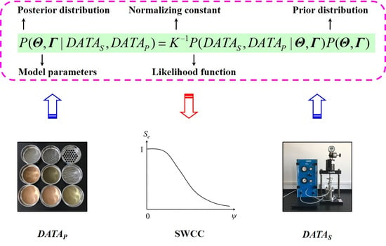
The plausibility of possible $\Theta$ and $\Gamma$ can be evaluated by the posterior distribution $P(\Theta ,\Gamma |DAT{A}_S,DAT{A}_P)$ based on the available test data (i.e., DATA_P, DATA_S) and prior knowledge under Bayesian framework. According to the Bayes’ theorem, $P(\Theta ,\Gamma |DAT{A}_S,DAT{A}_P)$ is written as (e.g., [24,29,30]):

$$P(\Theta ,\Gamma |DAT{A}_S,DAT{A}_P)=K^{-1}P(DAT{A}_S,DAT{A}_P|\Theta ,\Gamma )P(\Theta ,\Gamma )\hspace{0.33em}$$

(9)

where $K=P(DAT{A}_S,DAT{A}_P)={\displaystyle \int P(DAT{A}_S,DAT{A}_P|\Theta ,\Gamma )P(\Theta ,\Gamma )d\Theta d\Gamma }$ is a normalizing constant; $P(DAT{A}_S,DAT{A}_P|\Theta ,\Gamma )$ is likelihood function describing the goodness-of-fit of model predictions with the test data DATA_S and DATA_P for a given set of $\Theta$ and $\Gamma$; $P(\Theta ,\Gamma )$ is prior distribution of $\Theta$ and $\Gamma$. Using the conditional probability formula, $P(DAT{A}_S,DAT{A}_P|\Theta ,\Gamma )$ is expressed as:

$$\begin{array}{ll}P(DAT{A}_S,DAT{A}_P|\Theta ,\Gamma )& =P(DAT{A}_S|DAT{A}_P,\Theta ,\Gamma )\times P(DAT{A}_P|\Theta ,\Gamma )\\ & =P(DAT{A}_S|\Theta )\times P(DAT{A}_P|\Theta ,\Gamma )\end{array}$$

(10)

Assuming that errors of ${\epsilon }_S$ and ${\epsilon }_P$ in different data points are statistically independent, $P(DAT{A}_S|\Theta )$ and $P(DAT{A}_P|\Theta ,\Gamma )$ can be given by (e.g., [24,25,28]):

$$\begin{array}{ll}P(DAT{A}_S|\Theta )& ={\left(2\pi \right)}^{-\frac{N_S}{2}}{\sigma }_{{\epsilon }_S}^{-N_S}\exp \left[-\frac{N_S}{2{\sigma }_{{\epsilon }_S}^2}{J}_S(\Theta |DAT{A}_S)\right]\\ & \hspace{0.33em}={\left(2\pi \right)}^{-\frac{N_S}{2}}{\sigma }_{{\epsilon }_S}^{-N_S}\exp \left[-\frac{1}{2{\sigma }_{{\epsilon }_S}^2}{\displaystyle \sum _{i=1}^{N_S}{(S_{e,i}-S_{e,i}^m)}^2}\right]\end{array}$$

(11)

$$\begin{array}{ll}P(DAT{A}_P|\Theta ,\Gamma )& ={\left(2\pi \right)}^{-\frac{N_P}{2}}{\sigma }_{{\epsilon }_P}^{-N_P}\exp \left[-\frac{N_P}{2{\sigma }_{{\epsilon }_P}^2}{J}_P(\Theta ,\Gamma |DAT{A}_P)\right]\\ & ={\left(2\pi \right)}^{-\frac{N_P}{2}}{\sigma }_{{\epsilon }_P}^{-N_P}\exp \left[-\frac{1}{2{\sigma }_{{\epsilon }_P}^2}{\displaystyle \sum _{t=1}^{N_P}{(P_t-P_t^m)}^2}\right]\end{array}$$

(12)

where $J_S(\Theta |DAT{A}_S)$ and $J_P(\Theta ,\Gamma |DAT{A}_P)$ are the goodness-of-fit function. Substituting Equations (11) and (12) into Equation (10), $P(DAT{A}_S,DAT{A}_P|\Theta ,\Gamma )$ is reformulated as:

$$\begin{array}{ll}P(DAT{A}_S,DAT{A}_P|\Theta ,\Gamma )=& (2\pi {)}^{-\frac{N_S}{2}}{\sigma }_{{\epsilon }_S}^{-N_S}\exp \left[-\frac{1}{2{\sigma }_{{\epsilon }_S}^2}{\displaystyle \sum _{i=1}^{N_S}{(S_{e,i}-S_{e,i}^m)}^2}\right]\times \\ & {\left(2\pi \right)}^{-\frac{N_P}{2}}{\sigma }_{{\epsilon }_P}^{-N_P}\exp \left[-\frac{1}{2{\sigma }_{{\epsilon }_P}^2}{\displaystyle \sum _{t=1}^{N_P}{(P_t-P_t^m)}^2}\right]\end{array}$$

(13)

The $P(\Theta ,\Gamma )$ indicates the available information on $\Theta$ and $\Gamma$ when test data is lacking (e.g., [30]). For illustration, a joint uniform distribution of $\Theta$ and $\Gamma$ is adopted as the prior distribution in this study which requires determination of the ranges of $\Theta$ and $\Gamma$. Thus, $P(\Theta ,\Gamma )$ is expressed as:

$$P(\Theta ,\Gamma )\hspace{0.33em}=\left\{\begin{array}{ll}1& {\Theta }_i\in [{\mathsf{\Theta }}_i^{\min },\hspace{0.33em}{\Theta }_i^{\max }],\hspace{0.33em}i=1,\hspace{0.33em}2,\hspace{0.33em}\dots ,\hspace{0.33em}{N}_a\\ \overline{({\Theta }_i^{\max }-{\Theta }_i^{\min })({\Gamma }_j^{\max }-{\Gamma }_j^{\min })}& {\Gamma }_j\in [{\Gamma }_j^{\min },\hspace{0.33em}{\Gamma }_j^{\max }],\hspace{0.33em}j=1,\hspace{0.33em}2,\hspace{0.33em}\dots ,\hspace{0.33em}{N}_b\\ 0& \mathrm{others}\end{array}\right.$$

(14)

where the superscript “max” and “min” denote the maximum value and minimum value, respectively; Θ_i represents the i-th element in $\Theta$; Γ_j represents the j-th element in $\Gamma$; N_a and N_b are the number of elements in $\Theta$ and $\Gamma$, respectively.

After deriving the likelihood function and prior distribution, solving the posterior distribution $P(\Theta ,\Gamma |DAT{A}_S,DAT{A}_P)$ is of primary concern. Generally, it is a non-trivial task to calculate $P(\Theta ,\Gamma |DAT{A}_S,DAT{A}_P)$ using direct numerical integration method, which involves a multi-dimensional integration with respect to $\Theta$ and $\Gamma$ (i.e., Equation (9)). In such a case, Markov chain Monte Carlo simulation (MCMCS) method offers a viable way to solve the posterior distribution in an efficient manner, which has been widely used in geotechnical engineering for parameter identification and model comparison (e.g., [31,32]). Among several MCMCS algorithms and their variants, Metropolis–Hastings (M–H) algorithm (e.g., [33,34]) has gained popularity in geotechnical engineering due to its conceptual simplicity (e.g., [29,35]).

The preliminary stage of M–H algorithm is to generate a Markov Chain that contains a sequence of random samples of target variables (e.g., $\Theta$ and $\Gamma$) generated from a predefined proposal probability density function (PDF), where candidate samples are selected or not according to the accept ratio. When the Markov chain satisfies its stationary condition, the associated MCMCS samples can be applied to portray the target PDF (e.g., $P(\Theta ,\Gamma |DAT{A}_S,DAT{A}_P)$). Details of the M–H algorithm are omitted here for the sake of brevity, which can be referred to Wang and Cao [31]. The major merit of M–H algorithm is that there is no need to calculate a multi-dimensional integration underlying K, thus bypassing the computational complexity encountered in calculating the posterior distribution under Bayesian framework. Thus, the M–H algorithm is used in this study to identify the AP model parameters $\Gamma$ and the SWCC model parameters $\Theta$.

A large number of MCMCS samples of $\Theta$ and $\Gamma$ are firstly generated from the posterior distribution (i.e., Equation (9)) using M–H algorithm, and subsequently conventional statistical analyses are conducted to evaluate the posterior statistics (e.g., mean values and standard deviations) and distributions (e.g., PDFs) of $\Theta$ and $\Gamma$. The implementation procedure described above is discussed in the next section.

3. Implementation Procedure

Generally, the implementation of the proposed approach involves 5 steps. Details of each step and the corresponding equations are summarized as follows:

(1) Obtain the available PSD test data DATA_P = {($P_t^m$, $D_t$), t = 1, 2,…, N_P } and DATA_S = {($S_{e,i}^m$, ${\psi }_{s,i}$), i = 1, 2,…, N_S} from direct measurements;

(2) Determine possible ranges of model parameter $\Theta$ and $\Gamma$ from previous literatures, which are needed in Equation (14) to specify the prior knowledge;

(3) Use M–H algorithm to simulate a number $N_{MH}$ of MCMCS samples of $\Theta$ and $\Gamma$ based on Equation (9);

(4) Calculate the posterior statistics (e.g., the most probable values (MPVs) and distributions (e.g., marginal PDFs) of $\Theta$ and $\Gamma$ of interest with the aid of conventional statistical analyses;

(5) Estimate SWCC using the parametric model with its corresponding MPVs of $\Theta$.

The five steps summarized above can be programmed as a user function or toolbox in commonly used software (e.g., MATLAB (R2014a, The MathWorks, Inc, Natick, MA, USA)), so as to facilitate its application in geotechnical engineering practice. The proposed approach and its implementation procedure described above are illustrated using real test data contained in UNSODA, as discussed in the next section.

4. Illustration Using Test Data Contained in UNSODA

In this section, the proposed approach is employed to predict SWCC using the test data in the unsaturated soil hydraulic database of UNSODA. The UNSODA established by U.S. Department of Agriculture (USDA) contains a total of 790 soil samples, which can be categorized into 12 soil classes by virtue of the USDA soil conservation service classification scheme. It plays a significant role in sharing the measured hydraulic data to public, which contains various types of test data measured from in-situ and/or laboratory tests, such as hydraulic data (i.e., volumetric water content, hydraulic conductivity, and soil water diffusivity), particle-size distribution data, bulk density, and organic matter content (e.g., [36,37]). In this study, the test data of particle-size distribution and volumetric water content are used in the proposed approach.

The typical ranges of model parameters required in the definition of prior distribution are tabulated in

Table 1. Typical ranges of model parameters.

Model Parameters	Typical Ranges
αf	(0 kPa, 20 kPa]
nf	(0, 10]
mf	(0, 20]
αAP	(1, 5]
${\sigma }_{{\epsilon }_S}$, ${\sigma }_{{\epsilon }_P}$	(0, 1]

. These typical ranges are determined from the published literatures (e.g., [1,20]). The standard deviations of ${\sigma }_{{\epsilon }_S}$ and ${\sigma }_{{\epsilon }_P}$ are deemed to vary from 0 to 1, which are the theoretical bounds of the effective degree of saturation and percentage passing. As mentioned in the preceding section, it is necessary to determine the hypothetical number of fractions firstly when using AP model to predict the SWCC. Arya and Paris [6] suggested that it is reasonable to use N_P = 20, with the boundaries at particle diameters of 1, 2, 3, 5, 10, 20, 30, 40, 50, 70, 100, 150, 200, 300, 400, 600, 800, 1000, 1500, and 2000 μm. Following Arya and Paris [6], N_P = 20 is used in this study.

Based on the available test data (i.e., DATA_P and DATA_S) and the prior knowledge, M–H algorithm is conducted to generate 500,000 random samples of $\Theta$ and $\Gamma$. Then, these MCMCS samples can be used to evaluate the posterior statistics and distributions of interest. Firstly, the proposed approach is validated using the test data of soil code 3190 in UNSODA. Secondly, the performance of the proposed approach, Arya et al. [5] model, Vaz et al. [21] model, Mohammadi and Vanclooster [9] model, Arya and Heitman [4] model in predicting SWCC are compared based on three sets of test data (i.e., soil code 2201, 3190, and 4180). Thirdly, the accuracy of the proposed approach in high soil suction range is explored. Finally, the proposed approach is applied to determine the scaling parameter using test data of each soil sample in UNSODA.

4.1. Validity of the Proposed Approach

To validate the accuracy of the proposed approach, the cross-validation technique is used in this study, where the available test data are divided into two subsets. One subset used to calibrate the proposed approach and the other subset used to test the proposed approach [38], which are referred to as training dataset and testing dataset, respectively. For illustration, a soil sample, namely soil code 3190 in UNSODA, is used herein. The soil sample belongs to loam and has 11 data points. Choose a training dataset containing 9 data points from these data, and the other two data points are regarded as testing dataset. Subsequently, the proposed approach is performed to determine the SWCC based on the training dataset and prior knowledge. The estimated SWCC obtained from the proposed approach is then compared with the testing dataset to explore the validity of the proposed approach. In this example, five possible combinations of the training dataset and the testing dataset are investigated.

Figure 2 plots the results obtained from cross-validation using test data of soil code 3190 in UNSODA. It is shown that the estimated SWCC, namely the most probable FX model (i.e., FX model with its corresponding MPVs of $\Theta$), obtained from the proposed approach (see red line) agrees well with the training dataset (see open circles). This implies that the proposed approach portrays the SWCC of the training dataset reasonably well in this example, and properly determines the SWCC using the available test data. For validation, Figure 2 also includes the testing dataset (see open triangles) selected from the test data. It is found that the most probable FX model obtained from the proposed approach provides accurate estimates of the SWCC compared with the testing dataset. For five different cases shown in Figure 2, the most probable FX model is generally consistent with the training dataset and the testing dataset. Such agreement validates the proposed approach.

4.2. Comparison with Different Methods

To further validate the proposed approach, a comparative study is conducted in this section to explore the effectiveness of the proposed approach with Arya et al. [5] model, Vaz et al. [21] model, Mohammadi and Vanclooster [9] model (MV), and Arya and Heitman [4] model (AH). For illustration, three sets of test data are selected from UNSODA, namely soil code 2201, 3190, and 4180, which are belongs to sand, loam, and silt loam, respectively. For soil code 2201 of sand, Arya et al. [5] suggested a constant value of 1.285 of the scaling parameter α_AP for sand. Substituting α_AP = 1.285 into Equation (5) provides the pressure head, and the corresponding volumetric water content is subsequently obtained using Equation (6), as shown in Figure 3a. It is found that there is a significant discrepancy between the real test data (see open circles) and the corresponding predictions obtained from Arya model. This discrepancy may be due to the variability of α_AP for different soil samples, indicating that the constant value of 1.285 is not applicable for all sand soils. Under such circumstances, a mathematical equation proposed by Vaz et al. [21] is used to relate the α_AP to the volumetric water content $\theta$ (i.e., ${\alpha }_{AP}=0.947+0.427\exp (-\theta /0.129)$), so as to avoid treating α_AP as a constant. Figure 3a also plots the predictions of SWCC using Vaz model (i.e., the mathematical equation), it is shown that Vaz model tends to underestimate the SWCC. This may be attributed to the fact that the accuracy of Vaz model is highly dependent on the database used for calibration, leading to misleading estimates of SWCC for soils outside the calibrated database. To bypass the difficulty in determining the empirical coefficients (e.g., α_AP), two conceptual models are developed by Mohammadi and Vanclooster [9] and Arya and Heitman [4]. Their corresponding estimates of SWCC are included in Figure 3a, the results seem to be unsatisfactory compared with the test data. Such unsatisfactory performance may be caused by the simplified soil structure assumption underlying the MV model and AH model. In contrast, the proposed approach is able to provide proper estimates of SWCC by making use of available test data, as shown in Figure 3a with solid black line.

Similar observations are also found for the soil code 3190 and 4180, as shown in Figure 3b,c. In general, the proposed approach outperforms the other four methods (i.e., Arya, Vaz, MV, and AH model) in predicting the SWCC. The accuracy of Arya model and Vaz model depends on the calibrated database used for calibration, which limits their applicability to the soils outside the calibrated database. Although MV model and AH model are no longer rely on empirical parameters, the simplified soil structure assumption weakens their validity in practical applications. In such a case, the proposed approach offers a rational way to systemically combine information from available test data for properly predicting the SWCC.

4.3. Predicting SWCC in the High Suction Range

Generally, a limited number of data points instead of a complete SWCC are typically obtained from direct measurements. Thus, it is difficult to perform a complete measurement of SWCC over a wide range of soil suction (i.e., 0–10⁶ kPa) in engineering practice. To explore the predictive capability of the proposed approach in the high soil suction range, three sets of test data in UNSODA are used herein for illustration, namely soil code 2622, 2743, and 4620. Rahimi and Rahardjo [39] found that SWCC within the soil suction range of 100 kPa is available for most direct measurements. Therefore, the soil suction equaling to 100 kPa is regarded as a critical value in this example for dividing the test data into two parts. One part used for calibration and the other part used for validation. For soil code 2622, it belongs to clay and has a total of 11 data points, in which seven data points in the suction range of 0–100 kPa and the remaining four data points beyond the 100 kPa. Thus, the seven data points are used as training dataset and the other four data points are regarded as testing dataset. Figure 4a compares the predictions of SWCC calculated from the proposed approach with the corresponding test data. It is shown that the results evaluated from the proposed approach agree well with the testing data points (see open circles), implying that the proposed approach is able to provide reasonably accurate estimates of SWCC in the high suction range (i.e., >100 kPa).

Likewise, divide the test data of soil code 2743 and 4620 into training dataset and testing dataset. Then, the proposed approach is applied to determine the SWCC using the training dataset, and the estimated SWCC are compared with the testing dataset, as shown in Figure 4b,c. Similar observations are also found for the soil code 2743 and 4620. This indicates that the proposed approach is capable of predicting SWCC in the high suction range, thus bypassing the difficulty in measuring SWCC over the entire range of soil suction. The proposed approach assists engineers in predicting the SWCC in a relatively rational way and obtaining a complete SWCC in practice.

4.4. Ranges of Scaling Parameter for Different Soil Types in UNSODA

To further investigate the possible ranges of scaling parameter α_AP for different soil types, the proposed approach is applied to determine the scaling parameter of each soil sample in UNSODA. In this subsection, a total of 639 soil samples and 3753 PSD data points are retrieved from different types of soils in UNSODA.

Table 2. Ranges of scaling parameter for 12 soil types in UNSODA.

Soil Type	Number of Soil Samples	Number of PSD Data Points	Range of Scaling Parameter αAP
			Lower Bound	Upper Bound
sand (S)	152	1022	1.002	1.852
loamy sand (lS)	54	358	1.003	1.892
sandy loam (sL)	98	521	1.004	1.864
loam (L)	65	363	1.000	1.595
silt loam (SiL)	114	745	1.001	1.693
silt (Si)	3	18	1.067	1.174
sandy clay loam (scL)	47	243	1.019	1.789
clay loam (cL)	28	117	1.001	1.536
silt clay loam (sicL)	22	122	1.002	1.466
sandy clay (sC)	3	17	1.500	1.589
silt clay (siC)	14	64	1.010	1.516
clay I	39	163	1.004	1.682

tabulates the number of soil samples and the total number of data points for 12 soil types. For each soil type in UNSODA, data points of different soil samples are used to determine the scaling parameter separately in this study. Consider, for example, the sand soil contains a total of 152 soil samples. For each soil sample, the proposed approach is performed to identify the model parameters $\Theta$ and $\Gamma$, including scaling parameter and the associated fitting parameters of SWCC model (i.e., FX).

Figure 5a compares the predicted effective degree of saturation $S_e$ obtained from the proposed approach with the corresponding test data in UNSODA. For reference, the 1:1 line (i.e., predicted $S_e$ versus measured $S_e$) and linear regression line are also plotted in Figure 5a. It is shown that the majority of data points are gathered around the 1:1 line, indicating that the SWCC can be predicted reasonably well using the proposed approach. Besides, the coefficient of determination (i.e., R²) is applied to evaluate the performance of the proposed approach in predicting SWCC. The R² value of the regression line is 0.939, the high value of R² implies that the proposed approach can provide relatively accurate estimates of SWCC (e.g., [40,41]). Besides, a few data points deviate from the 1:1 line, such deviation may be attributed to the possible inconsistency between the test data of PSD and SWCC due to measurement errors. As a result, it is hard to strike a balance between them, namely, a set of model parameters (i.e., $\Theta$ and $\mathbf{\Gamma }$) to portray both of them well.

Similarly, the scaling parameters for the remaining 11 types of soils are also calculated, as shown in Table 2. In general, good agreements are also observed between the predicted and measured values of $S_e$, as shown in Figure 5b–l. The R² values of the regression line range from 0.833 (see Figure 5f) to 0.992 (see Figure 5k), indicating again that the proposed approach is able to provide relatively accurate predictions of SWCC for different soil types in UNSODA. Table 2 also summarizes the ranges of scaling parameter for each soil type obtained from the proposed approach. It is shown that the range of scaling parameter for a given soil type (e.g., α_AP $\in$ [1.002, 1.852], as shown in Table 2) is generally narrower than those used in this study for defining the joint uniform prior distribution (i.e., α_AP $\in$ (1, 5], as shown in Table 1). These ranges of 12 soil types not only can be used to determine the prior distribution of scaling parameter for further updating when new test data are available, but also offer engineers insights into the possible values of scaling parameter for different soil types.

5. Summary and Conclusions

This paper proposed a Bayesian approach to predict soil-water characteristic curve (SWCC) from particle-size distribution (PSD) based on the available test data and prior knowledge. The proposed approach identifies, simultaneously, scaling parameter in Arya and Paris (AP) model and fitting parameters of parametric SWCC model. Cross-validation technique was first used to investigate the validity of the proposed approach, and a comparative study was then performed. The predictive capability of the proposed approach in the high soil suction range was also explored. Finally, the proposed approach was applied to determine the scaling parameter of each soil sample in UNSODA. Major conclusions drawn from this study are given below:

(1) The proposed approach provides a proper prediction of SWCC by making use of the available test data and prior knowledge. The main advantage of the proposed approach lies in its facility in predicting SWCC based on the available test data, instead of collecting a large amount of test data from other sites for calibration. Thus, the proposed approach offers a viable way to systemically combine information from available test data for predicting SWCC with reasonable accuracy.

(2) The proposed approach is able to provide reasonably accurate estimates of SWCC in the high suction range (i.e., >100 kPa). Direct measurements of SWCC in the high soil suction range are generally time-consuming and costly. The proposed approach, as an alternative to direct measurements, is capable of predicting SWCC in the high suction range, bypassing the difficulty in measuring SWCC over the entire range of soil suction. It can assist engineers in obtaining a complete SWCC for geotechnical analyses involving unsaturated soils in practice.

(3) The predicted effective degree of saturation obtained from the proposed approach is generally in good agreement with the test data in UNSODA, indicating that the proposed approach can provide relatively accurate estimates of SWCC for different soil types in UNSODA. Besides, the ranges of scaling parameter for 12 soil types are also provided, which are narrower than those used in this study for defining the joint uniform prior distribution. These ranges not only can be used to determine the prior distribution of scaling parameter for further updating when new test data are available, but also offer practitioners insights into the possible values of scaling parameter for different soil types.

References

- Fredlund, D.G.; Rahardjo, H.; Fredlund, M.D. Unsaturated Soil Mechanics in Engineering Practice; John Wiley & Sons, Inc.: Hoboken, NJ, USA, 2012. [Google Scholar]
- Lu, N.; Likos, W.J. Unsaturated Soil Meichanics; John Wiley & Sons, Inc.: Hoboken, NJ, USA, 2004. [Google Scholar]
- Prakash, A.; Hazra, B.; Deka, A.; Sreedeep, S. Probabilistic Analysis of Water Retention Characteristic Curve of Fly Ash. Int. J. Geéomeéch. 2017, 17, 4017111. [Google Scholar] [CrossRef]
- Arya, L.M.; Heitman, J.L. A Non-Empirical Method for Computing Pore Radii and Soil Water Characteristics from Particle-Size Distribution. Soil Sci. Soc. Am. J. 2015, 79, 1537–1544. [Google Scholar] [CrossRef]
- Arya, L.M.; Leij, F.J.; Van Genuchten, M.T.; Shouse, P.J. Scaling Parameter to Predict the Soil Water Characteristic from Particle-Size Distribution Data. Soil Sci. Soc. Am. J. 1999, 63, 510–519. [Google Scholar] [CrossRef] [Green Version]
- Arya, L.M.; Paris, J.F. A Physicoempirical Model to Predict the Soil Moisture Characteristic from Particle-Size Distribution and Bulk Density Data. Soil Sci. Soc. Am. J. 1981, 45, 1023–1030. [Google Scholar] [CrossRef]
- Hwang, S.I.; Powers, S.E. Using Particle-Size Distribution Models to Estimate Soil Hydraulic Properties. Soil Sci. Soc. Am. J. 2003, 67, 1103–1112. [Google Scholar] [CrossRef]
- Li, D.F.; Gao, G.Y.; Shao, M.A.; Fu, B.J. Predicting available water of soil from particle-size distribution and bulk density in an oasis–desert transect in northwestern China. J. Hydrol. 2016, 538, 539–550. [Google Scholar] [CrossRef]
- Mohammadi, M.H.; Vanclooster, M. Predicting the Soil Moisture Characteristic Curve from Particle Size Distribution with a Simple Conceptual Model. Vadose Zone J. 2011, 10, 594–602. [Google Scholar] [CrossRef]
- Nasta, P.; Kamai, T.; Chirico, G.B.; Hopmans, J.W.; Romano, N. Scaling soil water retention functions using particle-size distribution. J. Hydrol. 2009, 374, 223–234. [Google Scholar] [CrossRef]
- Wösten, J.H.M.; Pachepsky, Y.A.; Rawls, W.J. Pedotransfer functions: Bridging the gap between available basic soil data and missing soil hydraulic characteristics. J. Hydrol. 2001, 251, 123–150. [Google Scholar] [CrossRef]
- Chiu, C.F.; Yan, W.M.; Yuen, K.V. Estimation of water retention curve of granular soils from particle-size distribution—A bayesian probabilistic approach. Can. Geotech. J. 2012, 49, 1024–1035. [Google Scholar] [CrossRef]
- Fredlund, M.D.; Wilson, G.W.; Fredlund, D.G. Use of the grain-size distribution for estimation of the soil-water characteristic curve. Can. Geotech. J. 2002, 39, 1103–1117. [Google Scholar] [CrossRef]
- Minasny, B.; McBratney, A.B.; Bristow, K.L. Comparison of different approaches to the development of pedotransfer functions for water-retention curves. Geoderma 1999, 93, 225–253. [Google Scholar] [CrossRef]
- Nemes, A.; Rawls, W.J. Evaluation of different representations of the particle-size distribution to predict soil water retention. Geoderma 2006, 132, 47–58. [Google Scholar] [CrossRef]
- Bouten, W.; Schaap, M.G. Modeling water retention curves of sandy soils using neural networks. Water Resour. Res. 1996, 32, 3033–3040. [Google Scholar] [CrossRef]
- Vereecken, H.; Maes, J.; Feyen, J.; Darius, P. Estimating the soil moisture retention characteristic from texture, bulk density, and carbon content. Soil Sci. 1989, 148, 389–403. [Google Scholar] [CrossRef]
- Chirico, G.; Medina, H.; Romano, N. Functional evaluation of PTF prediction uncertainty: An application at hillslope scale. Geoderma 2010, 155, 193–202. [Google Scholar] [CrossRef]
- Pachepsky, Y.; Rajkai, K.; Toth, B. Pedotransfer in soil physics: Trends and outlook—A review. Agrokém. Talajt. 2015, 64, 339–360. [Google Scholar] [CrossRef]
- Antinoro, C.; Bagarello, V.; Ferro, V.; Giordano, G.; Iovino, M. A simplified approach to estimate water retention for Sicilian soils by the Arya–Paris model. Geoderma 2014, 213, 226–234. [Google Scholar] [CrossRef]
- Vaz, C.M.P.; de Freitas Iossi, M.; de Mendonça Naime, J.; Macedo, Á.; Reichert, J.M.; Reinert, D.J.; Cooper, M. Validation of the Arya and Paris Water Retention Model for Brazilian Soils. Soil Sci. Soc. Am. J. 2005, 69, 577–583. [Google Scholar] [CrossRef]
- Fredlund, M.D.; Fredlund, D.G.; Wilson, G.W. An equation to represent grain-size distribution. Can. Geotech. J. 2000, 37, 817–827. [Google Scholar] [CrossRef]
- Bayat, H.; Rastgo, M.; Zadeh, M.M.; Vereecken, H. Particle size distribution models, their characteristics and fitting capability. J. Hydrol. 2015, 529, 872–889. [Google Scholar] [CrossRef]
- Yuen, K.V. Bayesian Methods for Structural Dynamics and Civil Engineering; John Wiley & Sons (Asia) Pte Ltd.: Singapore, 2010. [Google Scholar]
- Zhou, W.H.; Yuen, K.V.; Tan, F. Estimation of soil–water characteristic curve and relative permeability for granular soils with different initial dry densities. Eng. Geol. 2014, 179, 1–9. [Google Scholar] [CrossRef]
- Fredlund, D.G.; Xing, A. Equations for the soil-water characteristic curve. Can. Geotech. J. 1994, 31, 521–532. [Google Scholar] [CrossRef]
- Sillers, W.S.; Fredlund, D.G. Statistical assessment of soil-water characteristic curve models for geotechnical engineering. Can. Geotech. J. 2001, 38, 1297–1313. [Google Scholar] [CrossRef]
- Wang, L.; Cao, Z.J.; Li, D.Q.; Phoon, K.K.; Au, S.K. Determination of site-specific soil-water characteristic curve from a limited number of test data—A bayesian perspective. Geosci. Front. 2018, 9, 1665–1677. [Google Scholar] [CrossRef]
- Beck, J.L.; Au, S.-K. Bayesian Updating of Structural Models and Reliability using Markov Chain Monte Carlo Simulation. J. Eng. Mech. 2002, 128, 380–391. [Google Scholar] [CrossRef]
- Cao, Z.; Wang, Y. Bayesian model comparison and selection of spatial correlation functions for soil parameters. Struct. Saf. 2014, 49, 10–17. [Google Scholar] [CrossRef]
- Wang, Y.; Cao, Z.J. Probabilistic characterization of Young’s modulus of soil using equivalent samples. Eng. Geol. 2013, 159, 106–118. [Google Scholar] [CrossRef]
- Zhang, L.L.; Zhang, J.; Zhang, L.M.; Tang, W.H. Back analysis of slope failure with Markov chain Monte Carlo simulation. Comput. Geotech. 2010, 37, 905–912. [Google Scholar] [CrossRef]
- Hastings, W.K. Monte Carlo sampling methods using Markov chains and their applications. Biometrika 1970, 57, 97–109. [Google Scholar] [CrossRef]
- Metropolis, N.; Rosenbluth, A.W.; Rosenbluth, M.N.; Teller, A.H.; Teller, E. Equation of State Calculations. J. Chem. Phys. 1953, 21, 1087–1092. [Google Scholar] [CrossRef]
- Au, S.K.; Beck, J.L. Estimation of small failure probabilities in high dimensions by subset simulation. Probab. Eng. Mech. 2001, 16, 263–277. [Google Scholar] [CrossRef] [Green Version]
- Leij, F.J.; Alves, W.J.; van Genuchten, M.T.; Williams, J.R. The UNSODA Unsaturated Soil Hydraulic Database User’s Manual; Version 1.0. Report No. EPA-600-R-96-095; Environmental Protection Agency: Cincinnati, OH, USA, 1996.
- Nemes, A.; Schaap, M.G.; Leij, F.J.; Wösten, J.H.M. Description of the unsaturated soil hydraulic database UNSODA version 2.0. J. Hydrol. 2001, 251, 151–162. [Google Scholar] [CrossRef]
- Buckland, S.T.; Hjorth, J.S.U. Computer Intensive Statistical Methods: Validation Model Selection and Bootstrap. Biometrika 1994, 50, 586. [Google Scholar] [CrossRef]
- Rahimi, A.; Rahardjo, H. New approach to improve soil-water characteristic curve to reduce variation in estimation of unsaturated permeability function. Can. Geotech. J. 2016, 53, 717–725. [Google Scholar] [CrossRef]
- Zhang, W.G.; Goh, A.T.C. Multivariate adaptive regression splines for analysis of geotechnical engineering systems. Comput. Geotech. 2013, 48, 82–95. [Google Scholar] [CrossRef]
- Zhang, W.G.; Goh, A.T.C. Multivariate adaptive regression splines and neural network models for prediction of pile drivability. Geosci. Front. 2016, 7, 45–52. [Google Scholar] [CrossRef] [Green Version]
Figure 1.
Comparison of the predicted soil-water characteristic curve (SWCC) obtained from Arya and Paris (AP) model applying different values of scaling parameter.
Figure 2.
Cross-validation results of soil code 3190 in Unsaturated Soil Database (UNSODA).
Figure 3.
Comparison of different indirect methods for predicting SWCC.
Figure 4.
Prediction of SWCC in the high suction range.
Figure 5.
Comparison of the predicted SWCC obtained from the proposed approach and its corresponding measured values in UNSODA.