On-Bottom Stability of Umbilicals and Power Cables for Offshore Wind Applications


1
The Faculty of Engineering, Østfold University College, Kobberslagerstredet 5, 1671 Kråkerøy, Fredrikstad, Norway
2
SINTEF Ocean, Marinteknisk Senter, Otto Nielsens vei 10, 7052 Trondheim, Norway
3
Department of Mechanical and Structural Engineering and Materials Science, University of Stavanger, 4036 Stavanger, Norway
*
Author to whom correspondence should be addressed.
Energies 2019, 12(19), 3635; https://doi.org/10.3390/en12193635
Submission received: 28 July 2019
/
Revised: 12 September 2019
/
Accepted: 19 September 2019
/
Published: 24 September 2019
(This article belongs to the Special Issue Recent Advances in Offshore Wind Technology)
Abstract
:With the increase in offshore wind farms, the demands for umbilicals and power cables have increased. The on-bottom stability of umbilicals and power cables under the combined wave and current loading is the most challenging design issue, due to their light weight and the complex fluid–cable–soil interaction. In the present study, the methodology for dynamic lateral stability analysis is first discussed; and the reliable hydrodynamic load model and cable–soil interaction model based on large experimental test data are described in detail. The requirement of the submerged weight of a cable to obtain on-bottom stability is investigated for three types of soil (clay, sand and rock), using the finite element program PONDUS, and the results are under the same load conditions. Several different aspects related to optimization design of the on-bottom stability are explored and addressed. There is a significant benefit for the on-bottom stability analysis to consider the reduction factors, due to penetration for clay and sand soil. The on-bottom stability is very sensitive to the relative initial embedment for clay and sand soil, due to the small diameter of the cables, and therefore, reliable prediction of initial embedment is required. In the energy-based cable–soil interaction model, the friction coefficient and the development of penetration affect each other and the total effect of friction force and passive resistance is complicated. The effect of the friction coefficient on the on-bottom stability is different from engineering judgement based on the Coulomb friction model. The undrained shear strength of clay is an important parameter for the on-bottom stability of umbilicals and cables. The higher the undrained shear strength of the clay, the larger the lateral displacement. Meanwhile, the submerged weight of sand has a minor effect on the lateral displacement of cables. The method used in the present study significantly improves the reliability of the on-bottom stability analysis of umbilicals and power cables for offshore wind application.
1. Introduction
Offshore wind farms can be essential in renewable energy policy and are an important element in the battle against climate change. They play a leading role in meeting renewable energy and carbon emission targets, and improve energy security for the future. In a new analysis released by the International Renewable Energy Agency (IRENA)—Innovation Outlook: Offshore Wind—offshore wind power has the potential to grow from 13 GW in 2015, to 100 GW in 2030 [1]. Floating wind technology has made great strides toward commercialization, with the world’s first floating offshore wind farm—Equinor’s Hywind Scotland Pilot Park—starting operation in 2017. The expected global capacity of floating offshore wind power is now up to 12 GW by 2030 [2]
In the oil and gas industry, a major design issue for any pipelines or flexibles is how to ensure that the product remains on the seabed where it was installed, as opposed to moving excessively laterally. This design facet is called on-bottom stability, which involves determining a submerged weight capable of withstanding hydrodynamic loads through friction and passive soil resistance, and it has long been an important study for offshore practice [3,4,5]. The failure of on-bottom stability of pipelines has recently been experienced in the Gulf of Mexico in the cases of hurricanes Katrina, Rita and Ivan, all of which caused extensive lateral displacements (in the order of kilometers) of pipelines, and collisions of pipelines with other subsea installations. The severe consequences are damage of the pipelines and considerable loss of production [6].
The main facilities of the offshore wind farm are illustrated in the Wave Hub plant [7]. One of the technical and infrastructure challenges related to the floating offshore wind farm is the connection of the floating offshore wind farm grid. The distance from the shore and the availability of networks at the point of connection remain a potential bottleneck. However, as far as cable technology is concerned, the dynamic section of the cables (the section that has to move) is an important issue. The typical floating electrical connections used in the floating offshore wind farm is described in Floating Electrical Connections [8]. In water depths of more than 100 m, the array cable layout also poses technical problems and a longer cable is needed for an array cable laid on the seabed. Both the array cable and the long-distance power cable connected to the shore will have the on-bottom stability problem. Studies of the dynamic response of cables and the evaluation of cost effective solutions need to be developed [9].
In offshore wind farms for both floating and non-floating wind turbines, umbilicals and power cables are widely used to control the system and transmit power from the offshore to grid, and they are exposed to a complex fluid–cable–soil interaction system after they are installed on seabed. One distinctive difference between the offshore wind farm and the onshore wind farm is the application of dynamic umbilicals and cables. The on-bottom stability of umbilicals and cables is a design challenge for the offshore wind industry and most of the designs are very conservative. The typical characteristics of umbilicals and power cables compared to traditional pipelines are small in diameter, lightweight and have a low bending stiffness. Due to these characteristics, umbilicals and power cables are prone to experience excessive lateral displacement, and then the on-bottom stability becomes more challenging. The excessive lateral displacement will cause the damage of umbilicals and power cables, collision with each other and the shutdown of wind farms. The reliable design of the on-bottom stability of umbilicals and power cables for offshore wind application is essential for the safety and integrity of the wind farms.
The engineering design method, which was originally developed for on-bottom stability analysis of pipelines with large diameters, generally consists the following four steps [10]:
- (1)
- Obtaining environmental data for 1-year, 10-year and 100-year conditions and seabed properties, which includes:
- -
- Water depth
- -
- Wave spectrum
- -
- Current velocity
- -
- Soil properties
- (2)
- Determining the hydrodynamic coefficients: drag, lift and inertia coefficients. These coefficients are dependent on Reynolds Number, Keulegan Number, steady current to wave ratio, and embedment.
- (3)
- Calculating the hydrodynamic forces, i.e., drag, lift and inertia forces.
- (4)
- Performing static force analysis at time step increments and assessing stability
A similar engineering method was also adopted in the offshore wind farm industry to check the absolute on-bottom stability of the umbilicals and power cables. However, it has proven to be difficult to meet absolute on-bottom stability requirement for umbilicals and power cables, due not only to the conservatism of engineering methods, but also because of the light submerged weight of umbilicals and power cables. In order to improve the design of the on-bottom stability for umbilicals and power cables, design criteria based on the allowable lateral displacement has been introduced, but this requires advanced time domain finite element method (FEM) simulation [11]. The deep offshore wind industry could benefit from the experience gained in the oil and gas sector. The exchange of knowledge with the oil and gas industry would help develop deep offshore wind farms faster and more cost effectively. In the present study, the methodology used in the advanced FEM method is first presented and the parameters which are the most important in the assessment of on-bottom stability for umbilicals and cables are identified. The optimization design based on the dynamic stability simulation is explored and discussed afterwards.
2. Methodology
The on-bottom stability of umbilicals and cables is a rather complex problem involving fluid–cable–soil interaction, and it requires both reliable hydrodynamic load models and appropriate cable–soil interaction models.
The existing hydrodynamic load models for a cylinder on the seabed was extensively investigated in Joint Industry Project: pipeline lateral stability (PILS JIP) [12]. The main conclusion was that the Wake II models [13] were promising, but not sufficiently mature to be implemented in design practice at present, and that the hydrodynamic load model based on the database from the Danish Hydraulic Institute (DHI) was still superior, as the DHI database is the only most comprehensive and thoroughly documented empirical dataset available. The hydrodynamic load model applied in the present study is based on the Fourier coefficient database derived through extensive experimental campaigns at DHI and documented by Sorenson et al. [14] and Bryndum et al. [15]. The model accounts for wake effects and force amplification after flow reversal, giving significantly improved force predictions compared to conventional constant-coefficient Morison formulations.
Several pipe–soil interaction models have been developed in past decades, and the energy-based pipe–soil interaction model developed by SINTEF Ocean is still regarded as the state-of-art for soil modeling in dynamic on-bottom stability analyses [16]. It has also been adopted in DNV-RP-F109 [17]. The energy-based soil model contains two main components: friction component (Coulomb force) and passive soil force component due to penetration. The model for passive soil force was developed by Verley and Sotberg [18] for sand, and by Verley and Lund [19] for clay. The mathematical model of the passive soil resistance was established by using dimensional analysis methods fitted to testing data from the PIPESTAB [20] and AGA [21] projects.
The hydrodynamic load model and the pipe–soil interaction model used in the present study are described in detail in the next two sections. Both of them were implemented in the finite element software PONDUS developed by SINTEF Ocean.
2.1. Hydrodynamic Model
The database force model is based on the Fourier decomposition of hydrodynamic forces, recorded in laboratory experiments with combined regular waves and a steady current for a range of conditions, with each condition defined through a combination of Keulegan–Carpenter number , current-to-wave ratio and relative surface roughness . Here T is the wave period; is the current velocity. The range of experimental parameters for the regular wave tests is presented in Table 1. For umbilicals and cables with a small diameter, Reynolds numbers are normally in the high end. For a stationary cylinder, the drag force and lift force are expressed as a sum of harmonic components:
where is the drag force for stationary cylinder; is the lift force for stationary cylinder; D is the outer diameter of the cylinder; is the amplitude of the regular-wave flow velocity; , , , , and are the Fourier coefficients and phase angles.
The wave velocity amplitude rather than the time varying sum of the wave flow velocity and current flow velocity are used in Equations (1) and (2). The time variation in the DHI Fourier coefficient model is accounted for through time-varying drag and lift coefficients, and the influence of a steady current component is accounted for in the Fourier coefficients.
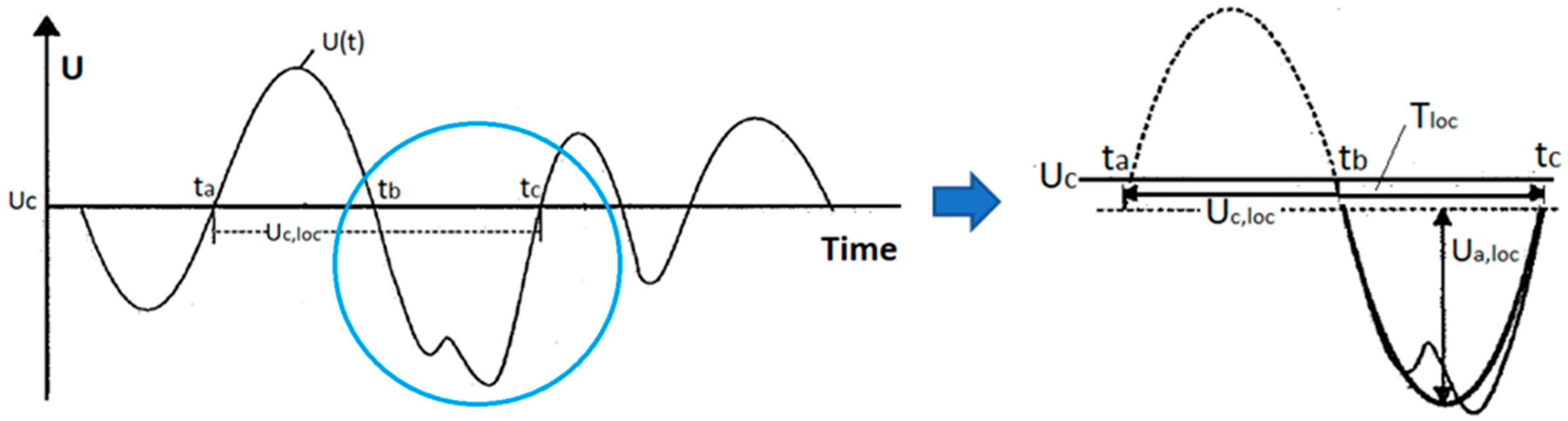
The time series of bottom wave velocities in irregular waves are decomposed into zero-upcrossing and zero-downcrossing half-wave cycles, with local wave parameters such as and , and each irregular half-cycle is treated as a regular wave, as shown in Figure 1. The appropriate local current velocity is found as . The local wave velocity amplitude is obtained by:
The horizontal and lift force for a stationary cylinder subjected to the fitted sinusoidal waves with velocity amplitude and period is given as:
where the constant inertia coefficient is .
Verley and Reed [22] proposed a method that enabled the use of the database force model of a stationary cylinder to a moving cylinder. In order to determine forces on the moving cylinder, it is necessary to determine the flow velocity near the cylinder (i.e., modified for the effects of the wake). The horizontal and lift forces on a stationary cylinder may be represented by:
where is the effective velocity.
Equations (6) and (7) are related to the force expressions given for the database force model in Equations (4) and (5), and the time dependent effective velocity is determined as:
where is the horizontal force from the database model, and and are constant coefficients assumed to be unaffected by the cylinder motion.
The total horizontal force on a moving cylinder may be expressed as:
The time-dependent lift force coefficient is given by:
The lift force on the moving cylinder is expressed as:
2.2. Soil Model
The main theory of the soil model is described in [23], and the lateral displacement of the cylinder is expressed as the sum of the elastic and plastic displacement:
where is the elastic displacement; is the plastic displacement.
In the elastic range, the soil force is presented as:
where is elastic soil stiffness (per unit length); is the soil damping constant.
In the plastic range, the soil force is expressed as a sum of friction force and passive soil resistance force as follows:
where if ; is the soil friction coefficient (); is the submerged weight of the umbilicals and power cables; is the lift force found from the hydrodynamic force model; is the passive resistance force function.
The transition from the elastic to the plastic range is defined as taking place when:
The transition from the elastic to the plastic range is defined as occurring when the cable velocity changes sign, that is, when .
The incremental form of the soil force in the elastic range is equal to:
The incremental form of the soil force in the plastic range is equal to:
where ().
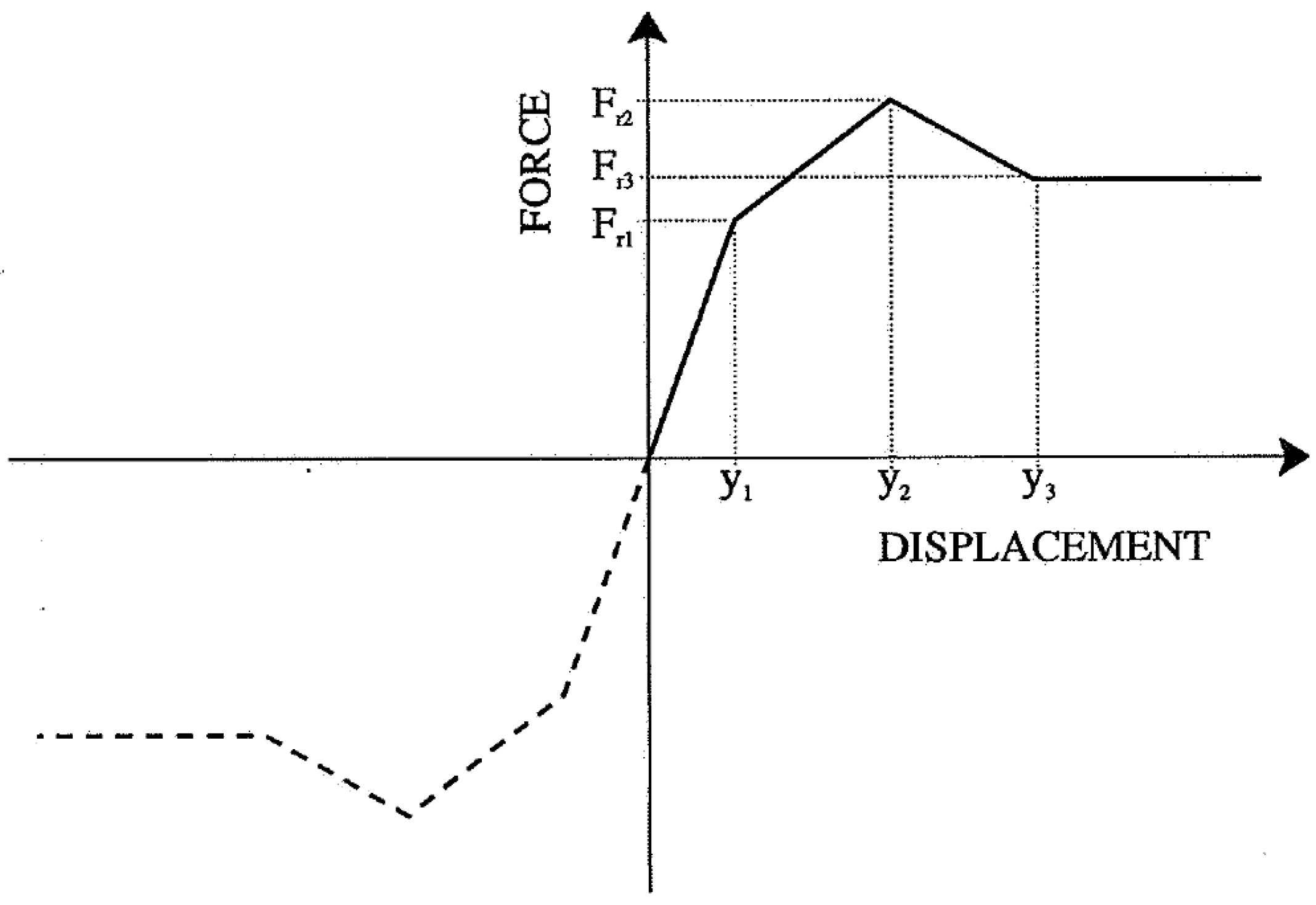
The soil force in the plastic range is computed in two steps. First, the cylinder penetration due to lateral movement is calculated, and then the corresponding force-displacement curve is determined. The force-displacement curve for the penetration dependent force is defined through the force levels , and and corresponding displacements , and as shown in Figure 2.
2.2.1. Sand Model
The initial embedment for the umbilicals and cables due to submerged weight , is given as:
where is the submerged weight of soil.
The breakout resistance force is given as:
where is the reference penetration for break-out (maximum pre-break-out penetration).
The frictional resistance and passive resistance are used to calculate the residual lateral resistance after the break-out. The equivalent penetration after the break-out is given as:
where is the maximum value of found in simulation up to the instant time considered.
If the cylinder continues to move in the same direction after the break-out, there is a horizontal resistance (in addition to the friction) due to a mound of soil being pushed ahead of the cylinder. The residual force has an effect on how far a cylinder section will move after the break-out while the cylinder motion is still in the same direction. The passive resistance after the breakout is calculated as:
The displacement , for which the maximum break-out force occurs, is set to 0.5D. The value of , i.e., where the resistance force becomes stable after the break-out, is taken as:
2.2.2. Clay Model
Initial penetration for the cable due to submerged weight, , is given by:
where ; ; is the submerged weight of clay; is the remolded undrained shear strength of soil.
The maximum break-out force corresponding to a given penetration z is taken as:
The point is determined through the expression:
where ; is the unit weight of water.
3. Dynamic On-Bottom Stability Simulation
In the present study, the finite element software PONDUS, developed by SINTEF Ocean, is used to perform the dynamic response of umbilicals and power cables, subject to the combined loadings of waves and current on a horizontal seabed. The main features of PONDUS are described in detail in [5].
The total length of the numerical model is 250 m with 50 elements. The recommended element length is 50 times that of the cylinder diameter. Dynamic analysis for 3 h of combined wave and current loads is performed. The application of different phase shifts between the harmonic wave components give rise to different time series realizations, with varying maximum wave height and sequence of waves, that both are important factors for the predicted maximum lateral displacement.
The design value is a very important parameter for the on-bottom stability analysis. A series of statistical analyses were performed during the establishment of the DNV RP F109. In DNV RP F109 the recommended design value is set to be the mean value plus one standard deviation of seven absolute maximum values from seven realizations. The statistical analyses are not performed for different set of seeds in the present paper, and the recommended value from DNV RP F109 is used to define the design value. Hence, seven analyses with random seeds are performed for each case. When the standard deviation in the resulting displacement has stabilized, the mean value plus the standard deviation is used as the design value.
3.1. Input Data
The datasheet of an umbilical is presented in Table 2, and the complex cross section of the umbilical is simplified to a cylinder with equivalent properties, also listed in Table 2. The equivalent thickness is calculated by obtaining approximately the same bending stiffness for the cylinder. The outer diameter remains the same and is the most important parameter in the calculation of hydrodynamic force and relative penetration during the lateral movement of the umbilical.
The environment data used in simulation are presented in Table 3. In this study, the load combination of 10-year current and 100-year waves is applied in the simulation.
As the current velocity is given at 1 m above the seabed, the mean perpendicular current velocity over the cylinder diameter is determined according to [17]:
where is the reference measurement height over seabed ( = 1 m); is the bottom roughness parameter.
In the present study, dynamic on-bottom stability of the umbilical is investigated for three different types of soil, and the mean perpendicular current over the cylinder diameter for clay, sand and rock seabed is presented in Table 4.
3.2. Analysis Matrix
The summary of the analysis for the three types of soil (clay, sand and rock) is presented in Table 5, Table 6 and Table 7. For clay, there are 25 cases named from C1 to C25, and for sand, a total 26 cases named from S1 to S26 are studied. Cases C4 and S4 are the base cases for the clay and the sand soil. The required submerged weight for these three types of soil, namely clay, sand and rock, is first investigated through the analysis of cases C1–C6, S1–S6 and R1–R6. Then the following parameter studies are performed:
(i) Reduction factors due to penetration for clay and sand soils
The force reduction due to penetration is not normally considered in the engineering design process, but it is perhaps important to include this effect for umbilicals and cables. Dynamic on-bottom analysis has the advantage of including the reduction factor due to penetration directly. The reduction factors and for horizontal and vertical loads due to penetration is given as [17]:
Cases C7–C12 and S7–S12 have the same input as C1–C6 and S1–S6, except that the reduction factor is not taken into account for C7–C12 and S7–S12. The effect of the reduction factor due to the penetration is investigated by comparing the analysis results between them.
(ii) Initial penetration for clay and sand soils
The initial penetration defines the initial condition for the umbilicals and the cables, and PILS JIP [16] stated that the prediction of the initial penetration needs to be further improved. In this study, the initial penetration is gradually increased for C13 to C15, and S13 to S17. The maximum initial penetration for the clay soil is 2 times of the base C4 and the maximum initial penetration for the sand soil is 3 times of the base S4. The effect of initial penetration on the maximum lateral displacement is investigated.
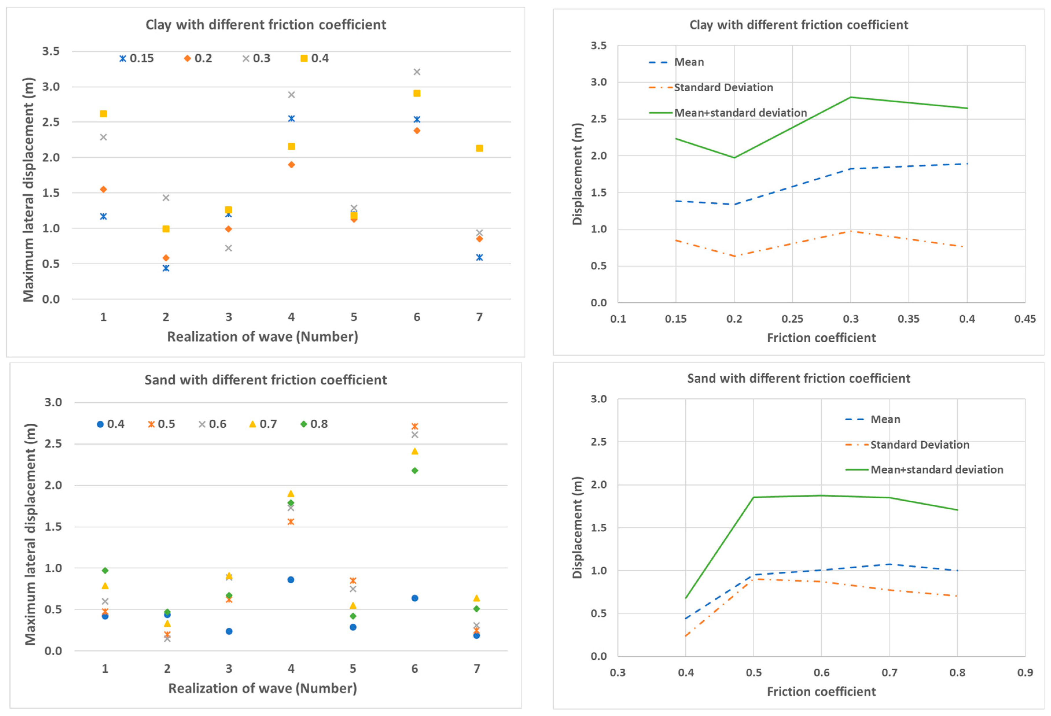
(iii) Friction coefficient of clay and sand soil
In engineering practice, when only the Coulomb friction model is considered, the conclusion is that the higher friction coefficient is, then the more stable the cylinder is.
When considering the energy-based soil model, the penetration is related to the accumulated displacement of the cylinder. The smaller the friction coefficient is, the earlier the cylinder starts to move. Moreover, both the accumulated displacement and the development of the penetration become larger as the friction coefficient decreases. The combined effect from the friction force and the passive resistance force means that the development of lateral displacement varies for different friction coefficients and does not have a certain trend corresponding to different friction coefficients [5]. In DNV-RP-F109 [17], the friction coefficient of sand and clay is set to be 0.6 and 0.2, respectively. In the present study, the effect of the friction coefficient is further investigated for the clay, with the friction coefficient range of 0.15–0.4 (case C16–C18), and for the sand, with friction coefficient range of 0.4–0.8 (case S18–S21).
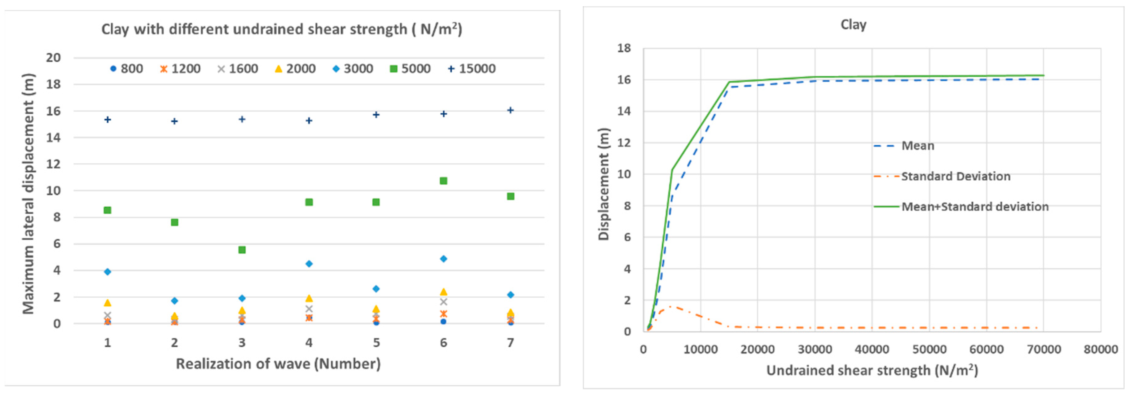
(iv) Undrained shear strength of clay
The undrained shear strength of clay represents the hardness of the soil, i.e., the lower the value, the softer the clay. The effect of undrained shear strength of clay is investigated for a range of 800 (soft clay) to 70,000 N/m2 (hard clay).
(v) Submerged unit weight of sand
The submerged weight of sand represents the compactness of sand, i.e., the lower the value, the looser the sand. The effect of the submerged unit weight of sand is investigated for the range of 6500 to 10,000 KN/m3 which corresponds to the loose and compact sand, respectively.
4. Results and Discussion
4.1. Required Submerged Weight of Umbilical
On a general form the design criteria for lateral stability is expressed as:
where is the allowable lateral displacement scaled to the cylinder diameter. When other limit states, e.g., the maximum bending and fatigue, are not investigated, the design criteria could be set as that the sum of the lateral displacement in the temporary condition, and during operation is less than 10 times of the cylinder diameter [17]. The design criteria used in the present study is 1.78 m.
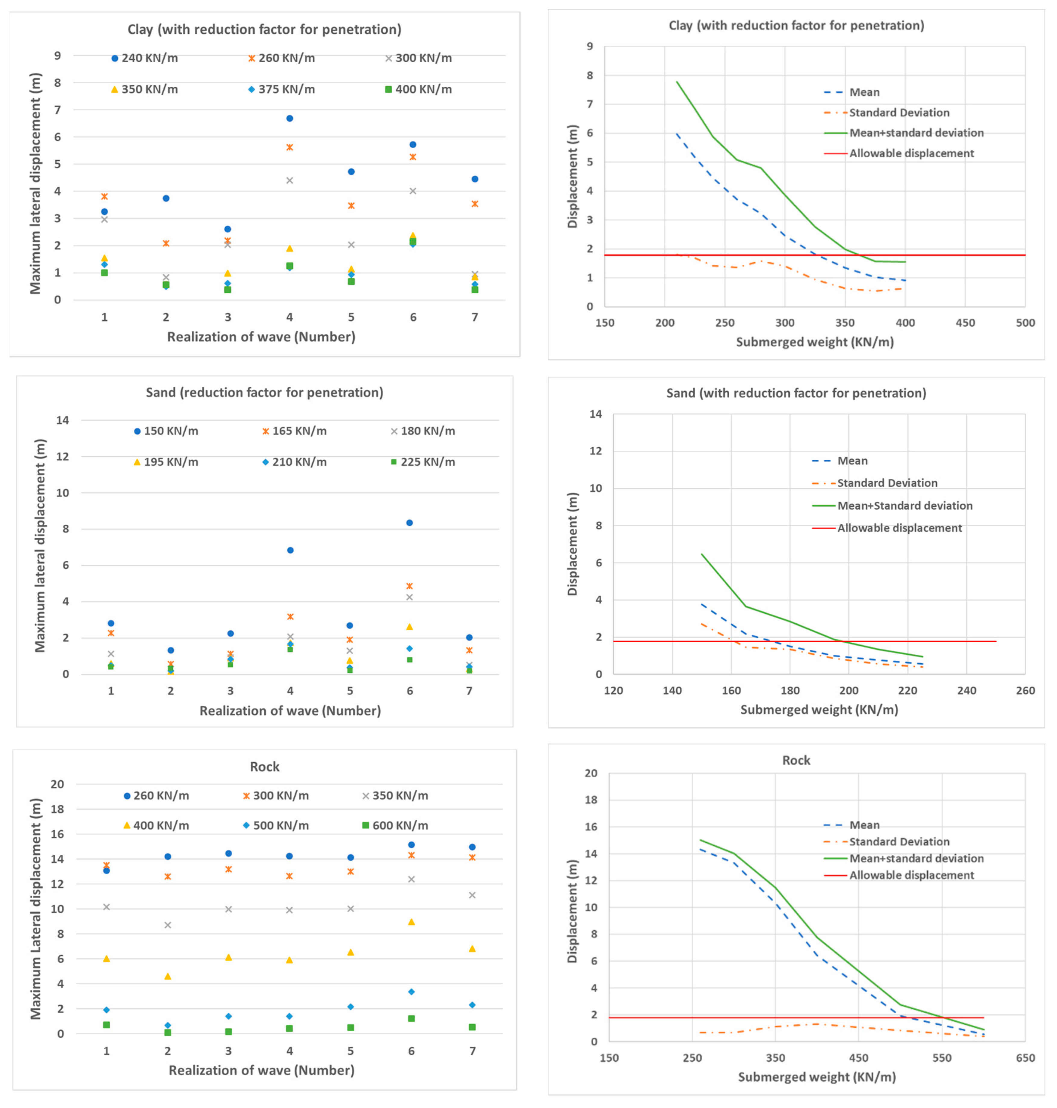
The maximum lateral displacements of an umbilical for seven wave realizations are shown in Figure 3 for clay, sand and rock seabed. The lateral displacements of seven realizations for each submerged weight are rather scattered, with high standard deviation for both the clay and the sand soils, but these do not vary significantly as compared to that for the rock. For the clay soil, the range of the lateral displacement is between 0.58 and 2.38 for the submerged weight of 350 KN/m. For the sand soil, the range of the lateral displacement is between 0.15 and 2.61 for the submerged weight of 195 KN/m. The pipe–soil interaction models for clay and sand are highly nonlinear while the Coulomb friction model is used for rock. The mean displacement and one standard deviation are also shown in Figure 4 for the clay, the sand and the rock cases. The standard deviation for the sand is relatively high and is in same magnitude as the mean displacement. The relationship between the mean displacement plus one standard deviation and the submerged weight of the umbilical is nonlinear for the sand and the clay soils.
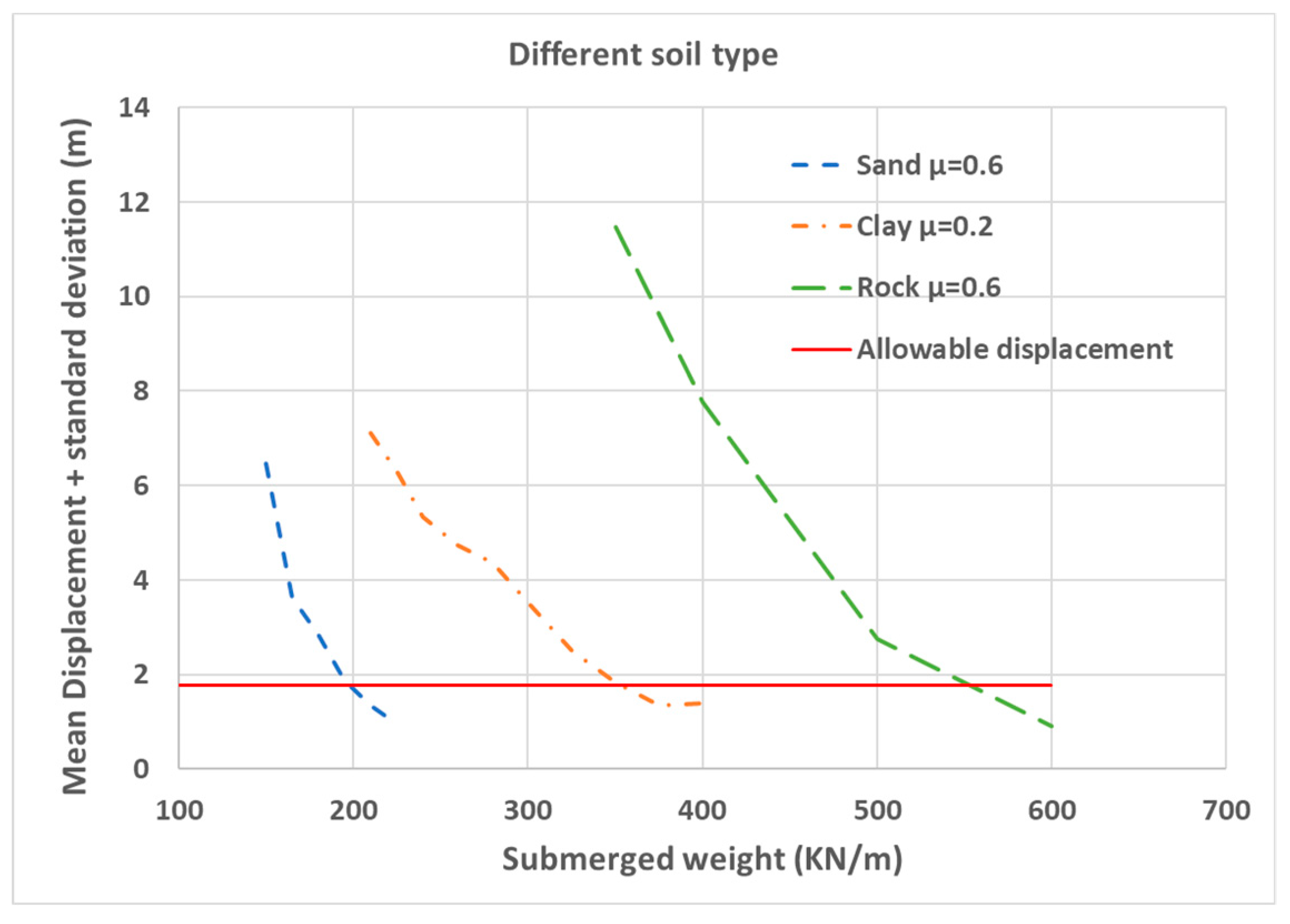
Under the same combined wave and current loading, the umbilical on the rock is most critical for on-bottom stability and it requires a submerged weight of 553 N/m to achieve the stable design, which is approximately 1.5 and 2.8 times that of the required submerged weight for the clay and the sand cases, respectively, as shown in Figure 4 and Table 8. The umbilical on the clay soil becomes stable when the submerged weight of the umbilical is larger than 362 N/m. The sand soil is the most favorable for the on-bottom stability in the present study, and the required submerged weight is 198 N/m.
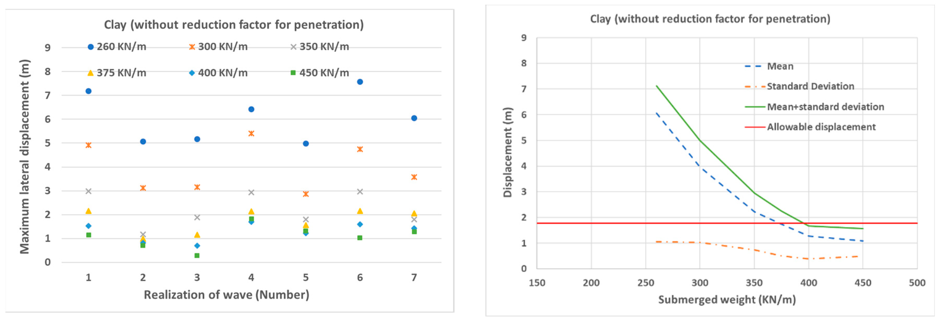
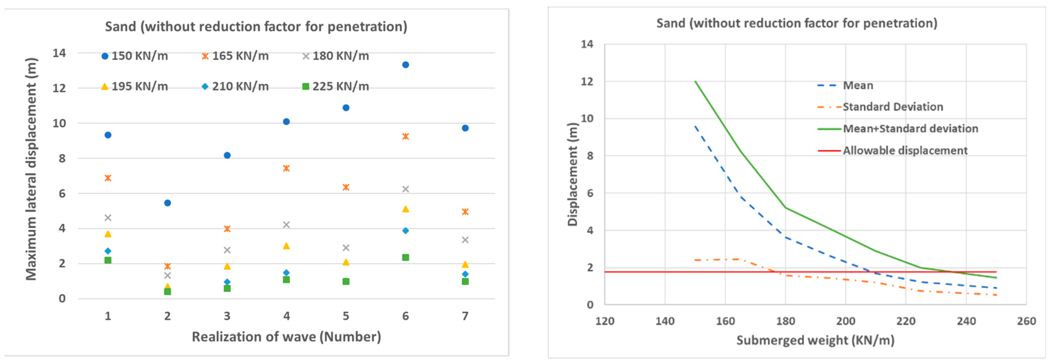
4.2. Load Reduction Due to Penetration
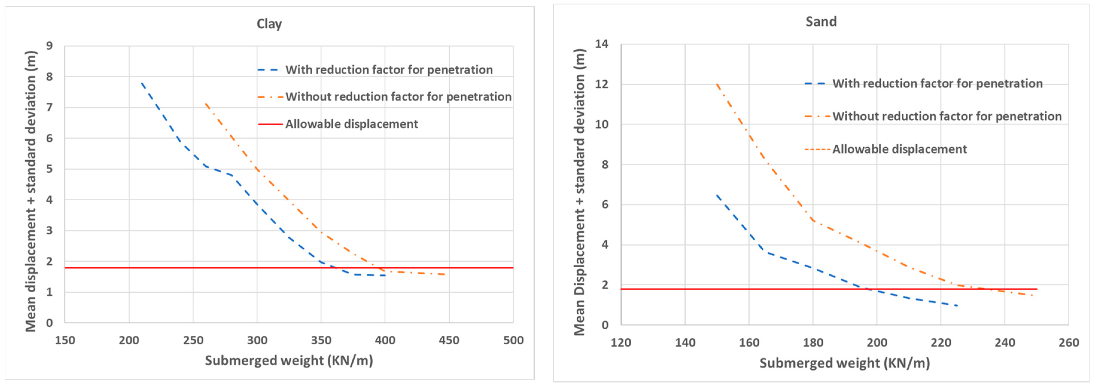
Figure 5 shows the lateral displacements for the cases which do not take into account the load reduction due to penetration, and these increase significantly, as compared to the cases with the load reduction. The comparisons of the mean displacement plus one standard deviation and the required submerged weight between the cases with and without load reduction factor are shown in Figure 6 and Table 9, respectively.
For the clay soil, the mean displacement plus one standard deviation of the cases without reduction factor increases approximately more than 40% for the submerged weights of 260, 350 and 375 KN/m. For the sand soil, the mean displacement plus one standard deviation of the cases without reduction factor increases approximately more than 100% for the submerged weights of 165, 195 and 225 KN/m. The reduction factor has a certain effect on the required submerged weight of umbilicals, and the required submerged weight increases approximately 9% and 18% for the clay and the sand soils, respectively. The load reduction due to the penetration needs to be considered in the on-bottom stability analysis of umbilicals and cables.
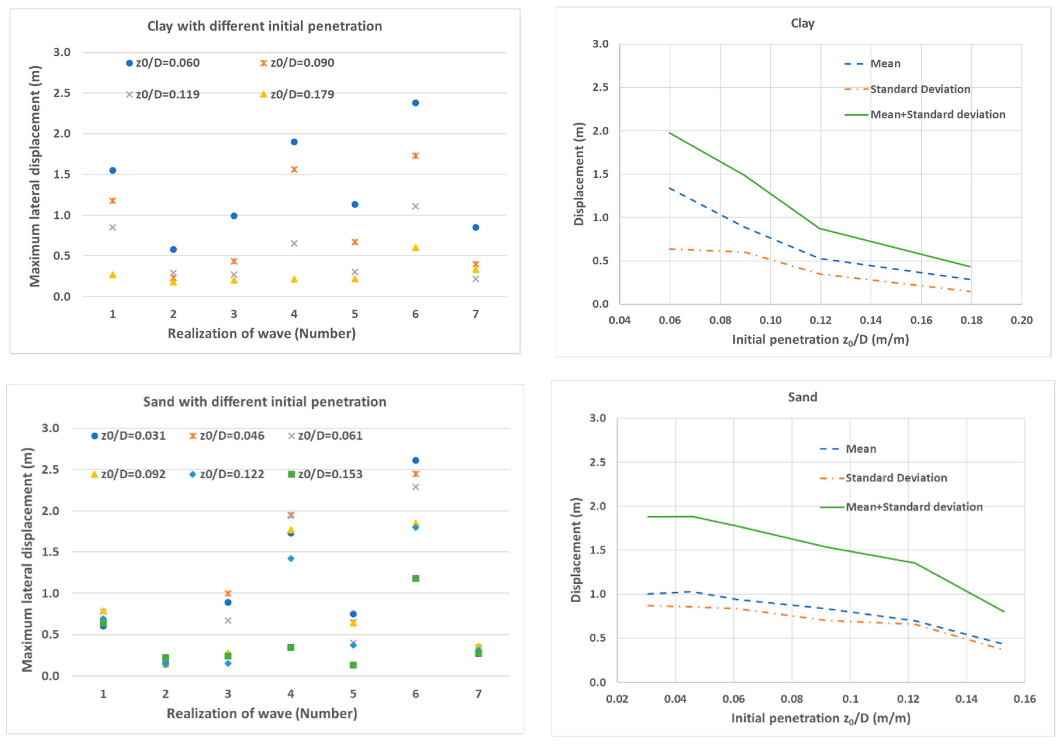
4.3. Initial Penetration
The analysis results with different initial penetration are shown in Figure 7 for both clay and sand cases. The initial penetration is an important parameter for the on-bottom stability analysis of umbilicals and cables. The lateral displacement of umbilicals reduces significantly when the initial penetration increases. For the clay soil, the mean displacement plus one standard deviation is reduced from 1.98 m to 0.43 m when the initial penetration increases from 0.06 to 0.179. For the sand soil, the mean displacement plus one standard deviation is reduced from 1.88 m to 0.80 m when the initial penetration increases from 0.031 to 0.153. The diameter of the umbilical is relatively small; and for the present study, when the absolute penetration increases one centimeter, the relative penetration will increase 0.056. The reliable model to predict the initial penetration for the umbilicals and cables with small diameter is necessary for on-bottom stability analysis.
4.4. Friction Coefficient
For the energy-based soil model, the influence of the friction coefficient on the lateral displacement is complicated. The total soil resistance force includes two components, i.e., friction force and passive resistance force due to the penetration. The friction coefficient will affect the development of the penetration and the result of the passive resistance force. The penetration becomes small when the friction coefficient increases, and this results in small passive resistance force. The combined resistance from the friction force and the passive resistance force will determine the development of the lateral displacement.
In the present study, the effect of friction coefficient does not show a clear trend and it is quite different from the engineering judgement based on the Coulomb friction model as shown in Figure 8. For the clay soil, Case C4, with a friction coefficient of 0.2, has the smallest mean displacement plus one standard deviation, and it means that the combined resistance from the friction force and the passive resistance force is less for the friction coefficients of 0.15, 0.3 and 0.4 when it is compared to the friction coefficient of 0.2. For the sand soil, Case S18, with a friction coefficient of 0.4, has the smallest mean displacement plus one standard deviation, and it means that the combined resistance is less for the friction coefficient of 0.5, 0.6, 0.7 and 0.8. It should be noted that DNV RP-F109 is based on the friction coefficient of 0.2 and 0.6 for clay and sand, respectively. According to the present study, it would not be conservative to use the friction coefficient of 0.2 for clay, if the friction coefficient varies in the range of 0.15 to 0.4.
4.5. Undrained Shear Strength of Clay
The undrained shear strength has a significant effect on the lateral displacement, as shown in Figure 9. The mean displacement plus one standard deviation increases from 0.28 m to 10.27 m when the undrained shear strength increases from 800 to 5000 N/m2. The initial penetration reduces significantly when the clay becomes harder, and this results in a smaller combined resistance and a larger lateral displacement. The umbilicals and cables tend to be more stable on soft clay than on hard clay.
4.6. Submerged Weight of Sand
The submerged weight of sand does not have a significant effect on the lateral displacement and the mean displacement plus one standard deviation increases slightly with the increasing of the submerged unit weight of sand, as shown in Figure 10.
5. Conclusions
In the present study, the on-bottom stability of umbilicals and power cables for offshore wind farms is investigated. In total, 57 simulations have been performed for clay, sand and rock seabed. The analysis results show that the design of umbilicals and power cables to meet the on-bottom stability requirement is challenging, due to their small diameter and flexibility. The main conclusions are given as follows:
- -
- For the same load combination, the sand soil is the most favorable for on-bottom stability and the rock is the most critical. The required submerged weight of the umbilical for the rock is approximately 1.5 and 2.8 times that for the clay and sand soils, respectively.
- -
- The reduction factor due to penetration reduces 9 to 18% of the required submerged weight for the clay and sand soils and improves the on-bottom stability. It should be considered in the design of the on-bottom stability through dynamic analyses.
- -
- The initial penetration has a significant effect on the on-bottom stability and the increases of absolute penetration by approximately a few centimeters will reduce 50% to 75% of the mean lateral displacement plus one standard deviation. The reliable model to predict the initial penetration of umbilicals and power cables is essential for the on-bottom stability analysis.
- -
- The effect of the friction coefficient on the on-bottom stability dose not match the common engineering judgement. The effect of friction is complicated and when the friction coefficient increases, then the competition between increased friction force and reduced passive resistance force will determine the final lateral displacement. In the present study, for the clay soil, the friction coefficient of 0.3 has the largest mean displacement plus one standard deviation; and for the sand soil, the friction coefficient of 0.5 has the largest mean displacement plus one standard deviation. In the design process, it is necessary to perform dynamic analysis to determine the critical friction coefficient for the on-bottom stability.
- -
- The undrained shear strength has a significant effect on the lateral displacement. The umbilicals and cables tend to be more stable on soft clay than on hard clay.
- -
- The submerged weight of sand does not have a significant effect on the lateral displacement of the umbilicals and cables.
- -
- The method used in the present study, not only significantly reduces the conservatism compared to the engineering methods, but also significantly improves the reliability of the on-bottom stability analysis for umbilicals and power cables in offshore wind application.
Author Contributions
The author contributions are listed as following: conceptualization, G.J., M.C.O.; methodology, G.J.; software, G.J.; formal analysis, G.J.; investigation, G.J., M.C.O.; writing—original draft preparation, G.J.; writing—review and editing, G.J., M.C.O.
Funding
This research received no external funding.
Conflicts of Interest
The authors declare no conflict of interest.
References
- International Renewable Energy Agency (IRENA). Innovation Outlook: Offshore Wind; IRENA: Abu Dhabi, United Arab Emirates, 2016; ISBN 978-92-95111-35-6. [Google Scholar]
- Carbon Trust. Floating Wind Joint Industry Project; Phase 1 Summary Report; Carbon Trust: London, UK, 2018. [Google Scholar]
- Guo, B.Y.; Song, S.H.; Chacko, J.; Ghalambor, A. Offshore Pipelines; Gulf Professional Publishing: Burlington, NJ, USA, 2005. [Google Scholar]
- Sumer, B.M.; Fredsøe, J. Hydrodynamic around Cylindrical Structures; World Scientific Publishing: Singapore, 2006. [Google Scholar]
- Ji, G.; Li, L.; Ong, M.C. On-Bottom stability analysis of subsea pipelines under combined irregular waves and currents. In Proceedings of the ASME 2017 36th International Conference on Ocean, Offshore and Arctic Engineering—Volume 5B: Pipelines, Risers, and Subsea Systems, Trondheim, Norway, 25–30 June 2017; ASME Press: New York, NY, USA, 2017. ISBN 978-0-7918-5770-0. [Google Scholar]
- Gagliano, M. Offshore pipeline stability during major storm events. In Proceedings of the Government/Industry Pipeline Research and Development Forum, New Orleans, LA, USA, 7–8 February 2007. [Google Scholar]
- Power Technology. The Cornwall Wave Energy Hub Project, UK. Available online: https://www.power-technology.com/projects/cornwallwaveenergyhu/ (accessed on 1 June 2019).
- Baring-Gould, I. Offshore Wind Plant Electrical Systems, Page 13 Floating Electrical Connections. Available online: https://www.boem.gov/NREL-Offshore-Wind-Plant-Electrical-Systems/ (accessed on 1 June 2019).
- Arapogianni, A.; Genachte, A.-B. Deep Water—The Next Step for Offshore Wind Energy; European Wind Energy Association: Brussels, Belgium, 2013. [Google Scholar]
- Palmer, A.C.; King, R.A. Subsea Pipeline Engineering; PennWell Corporation: Tulsa, OK, USA, 2008. [Google Scholar]
- Ji, G.; Li, L.; Ong, M.C. A comparison of simplified engineering and FEM methods for on-bottom stability analysis of subsea pipelines. In Proceedings of the ASME 2016 35th International Conference on Ocean, Offshore and Arctic Engineering OMAE 2016, Busan, Korea, 19–24 June 2016; OMAE Press: New York, NY, USA, 2016. [Google Scholar]
- JIP Pipeline Lateral Stability (PILS). Subsea Pipeline and Cable—Hydrodynamic Load Models; Document No.: 110JZMGH-6; DNV GL: Oslo, Norway, 2016. [Google Scholar]
- Aristodemo, F.; Tomasicchio, G.R.; Veltri, P. New model to determine forces at on-bottom slender pipelines. Coast. Eng. 2011, 58, 267–280. [Google Scholar] [CrossRef]
- Sorenson, T.; Bryndum, M.B.; Jacobsen, V. Hydrodynamic Forces on Pipelines—Model Tests; DHI Report No. L51522e; DHI: Hørsholm, Danmark, 1986. [Google Scholar]
- Bryndum, M.B.; Jacobsen, V.; Brand, L.P. Hydrodynamic forces from wave and current loads on marine pipelines. In Proceedings of the Offshore Technology Conference, Houston, TX, USA, 2–5 May 1983. [Google Scholar]
- JIP Pipeline Lateral Stability (PILS). Subsea Pipeline and Cable—Soil Resistance Models; Document No.: 110JZMGH-12; DNV GL: Oslo, Norway, 2017. [Google Scholar]
- DNV-RP-F109 On-Bottom Stability Design of Offshore Pipelines; DNV GL: Oslo, Norway, 2010.
- Verley, R.L.P.; Sotberg, T. A soil resistance model for pipelines placed on sandy soils. J. Offshore Mech. Arct. Eng. 1994, 116, 145–153. [Google Scholar] [CrossRef]
- Verley, R.L.P.; Lund, K.M. A soil resistance model for pipelines placed on clay soils. In Proceedings of the 14th International Conference on Offshore Mechanics and Arctic Engineering (OMAE 1995), Copenhagen, Denmark, 18–22 June 1995. [Google Scholar]
- Wolfram, W.R.; Getz, J.R.; Verley, R. PIPESTAB Project: Improved design basis for submarine pipeline stability. In Proceedings of the Offshore Technology Conference, Houston, TX, USA, 27–30 April 1987. [Google Scholar]
- Allen, D.W.; Lammert, W.F.; Hale, J.R.; Jacobsen, V. Submarine pipeline on-bottom stability: Recent AGA research. In Proceedings of the Offshore Technology Conference, Houston, TX, USA, 1–4 May 1989. [Google Scholar]
- Verley, R.L.P.; Reed, K. Use of laboratory force data in pipeline response simulations. In Proceedings of the 8th International Conference on Offshore Mechanics and Arctic Engineering (OMAE 1989), The Hague, The Netherlands, 19–23 March 1989. [Google Scholar]
- PONDUS. A Computer Program System for Pipeline Stability Design Utilizing a Pipeline Response Model Technical Manual; SINTEF Structures and Concrete: Trondheim, Norway, 1994. [Google Scholar]
Figure 1.
Decomposed time-series of wave velocity in irregular wave into half-cycle of a regular wave.
Figure 1.
Decomposed time-series of wave velocity in irregular wave into half-cycle of a regular wave.

Figure 2.
Force-displacement model for passive soil resistance .

Figure 3.
The lateral displacement of the umbilical for seven wave realizations and the mean and standard deviation of lateral displacement.
Figure 3.
The lateral displacement of the umbilical for seven wave realizations and the mean and standard deviation of lateral displacement.

Figure 4.
The mean displacement plus standard deviation for the clay, the sand and the rock cases.

Figure 5.
The lateral displacement of the umbilical for seven wave realizations and the mean and standard deviation of lateral displacement (cases without reduction factor).
Figure 5.
The lateral displacement of the umbilical for seven wave realizations and the mean and standard deviation of lateral displacement (cases without reduction factor).


Figure 6.
The mean displacement plus one standard deviation for the cases with/without reduction factor.
Figure 6.
The mean displacement plus one standard deviation for the cases with/without reduction factor.

Figure 7.
The lateral displacement of the umbilical for seven wave realizations and the mean and standard deviation of lateral displacement (with different initial penetration).
Figure 7.
The lateral displacement of the umbilical for seven wave realizations and the mean and standard deviation of lateral displacement (with different initial penetration).

Figure 8.
The lateral displacement of the umbilical for seven wave realizations and the mean and standard deviation of the lateral displacement (with different friction coefficients).
Figure 8.
The lateral displacement of the umbilical for seven wave realizations and the mean and standard deviation of the lateral displacement (with different friction coefficients).

Figure 9.
The lateral displacement of the umbilical for seven wave realizations and the mean and standard deviation of lateral displacement (with different undrained shear strength of clay).
Figure 9.
The lateral displacement of the umbilical for seven wave realizations and the mean and standard deviation of lateral displacement (with different undrained shear strength of clay).

Figure 10.
The lateral displacement of the umbilical for seven wave realizations and the mean and standard deviation of lateral displacement (with different submerged weight of sand).
Figure 10.
The lateral displacement of the umbilical for seven wave realizations and the mean and standard deviation of lateral displacement (with different submerged weight of sand).


Table 1.
Range of experimental parameters.
| Experimental Parameters | Test Range |
|---|---|
| Keulegan–Carpenter number | 2.5–160 |
| Current to wave velocity ratio | 0–1.6 |
| Surface roughness | {0.001, 0.01, 0.05} |
| Reynolds numbers | – |
Table 2.
Umbilical datasheet and equivalent properties.
| Datasheet | Equivalent Value Used in Simulation | |
|---|---|---|
| Outer diameter, (mm) | 178 | 178 |
| Thickness (mm) | - | 0.06 |
| Axial stiffness (N) | ||
| Bending stiffness (Nm2) |
Table 3.
Environment data.
| Environment Data | Return Period | |
|---|---|---|
| 10-year | 100-year | |
| Wave height Hs (m) | - | 14.8 |
| Wave period Tp (s) | - | 15.9 |
| Current velocity (m/s) (1 m above seabed) | 0.30 | - |
| Water depth (m) | 104 | |
Table 4.
Mean perpendicular current over cylinder diameter.
| Soil Type | ||
|---|---|---|
| Clay | 0.233 | |
| Sand | 0.219 | |
| Rock | 0.200 |
Table 5.
The overview of analysis cases for clay.
| Case | Submerged Weight of Umbilical (N/m) | Friction Coefficient | Load Reduction Factor | ||
|---|---|---|---|---|---|
| C1 | 240 | 0.2 | 2000 | 0.0439 * | Yes |
| C2 | 260 | 0.0467 * | |||
| C3 | 300 | 0.0524 * | |||
| C4 | 350 | 0.0598 * | |||
| C5 | 375 | 0.0636 * | |||
| C6 | 400 | 0.0675 * | |||
| C7 | 260 | 0.2 | 2000 | 0.0467 * | No |
| C8 | 300 | 0.0524 * | |||
| C9 | 350 | 0.0598 * | |||
| C10 | 375 | 0.0636 * | |||
| C11 | 400 | 0.0675 * | |||
| C12 | 450 | 0.0757 * | |||
| C13 | 350 | 0.2 | 2000 | 0.0897 ** | Yes |
| C14 | 0.1195 ** | ||||
| C15 | 0.1793 ** | ||||
| C16 | 350 | 0.15 | 2000 | 0.0598 * | Yes |
| C17 | 0.3 | ||||
| C18 | 0.4 | ||||
| C19 | 350 | 0.2 | 800 | 0.1203 * | Yes |
| C20 | 1200 | 0.0847 * | |||
| C21 | 1600 | 0.0690 * | |||
| C22 | 3000 | 0.0472 * | |||
| C23 | 5000 | 0.0360 * | |||
| C24 | 15,000 | 0.0207 * | |||
| C25 | 70,000 | 0.0000 * |
* Calculated by FEM program; ** Input to FEM program.
Table 6.
The overview of analysis cases for sand.
| Case | Submerged Weight of Umbilical (N/m) | Friction Coefficient | Submerged Unit Weight of Sand (KN/m3) | Load Reduction Factor | |
|---|---|---|---|---|---|
| S1 | 150 | 0.6 | 8203 | 0.0257 * | Yes |
| S2 | 165 | 0.0273 * | |||
| S3 | 180 | 0.0290 * | |||
| S4 | 195 | 0.0306 * | |||
| S5 | 210 | 0.0321 * | |||
| S6 | 225 | 0.0336 * | |||
| S7 | 150 | 0.6 | 8203 | 0.0257 * | No |
| S8 | 165 | 0.0273 * | |||
| S9 | 180 | 0.0290 * | |||
| S10 | 195 | 0.0306 * | |||
| S11 | 210 | 0.0321 * | |||
| S12 | 225 | 0.0336 * | |||
| S13 | 195 | 0.6 | 8203 | 0.0458 ** | Yes |
| S14 | 0.0611 ** | ||||
| S15 | 0.0917 ** | ||||
| S16 | 0.1222 ** | ||||
| S17 | 0.1528 ** | ||||
| S18 | 195 | 0.4 | 2000 | 0.0306 * | Yes |
| S19 | 0.5 | ||||
| S20 | 0.7 | ||||
| S21 | 0.8 | ||||
| S22 | 195 | 0.6 | 6500 | 0.0357 * | Yes |
| S23 | 7500 | 0.0324 * | |||
| S24 | 8500 | 0.0298 * | |||
| S25 | 9500 | 0.0277 * | |||
| S26 | 10,000 | 0.0268 * |
* Calculated by FEM program; ** Input to FEM program
Table 7.
The overview of analysis cases for rock.
| Case | Submerged Weight of Umbilical (N/m) | Friction Coefficient |
|---|---|---|
| R1 | 260 | 0.6 |
| R2 | 300 | |
| R3 | 350 | |
| R4 | 400 | |
| R5 | 500 | |
| R6 | 600 |
Table 8.
The required submerged weight.
| Soil Type | Required Submerged Weight of Umbilical (N/m) |
|---|---|
| Clay | 362 |
| Sand | 198 |
| Rock | 553 |
Table 9.
The required submerged weight (KN/m) for the cases with/without reduction factor.
| Soil Type | With Reduction Factor for Penetration | Without Reduction Factor for Penetration |
|---|---|---|
| Clay | 362 | 395 |
| Sand | 198 | 234 |
© 2019 by the authors. Licensee MDPI, Basel, Switzerland. This article is an open access article distributed under the terms and conditions of the Creative Commons Attribution (CC BY) license (http://creativecommons.org/licenses/by/4.0/).
Share and Cite
MDPI and ACS Style
Ji, G.; Ong, M.C. On-Bottom Stability of Umbilicals and Power Cables for Offshore Wind Applications. Energies 2019, 12, 3635. https://doi.org/10.3390/en12193635
AMA Style
Ji G, Ong MC. On-Bottom Stability of Umbilicals and Power Cables for Offshore Wind Applications. Energies. 2019; 12(19):3635. https://doi.org/10.3390/en12193635
Chicago/Turabian StyleJi, Guomin, and Muk Chen Ong. 2019. "On-Bottom Stability of Umbilicals and Power Cables for Offshore Wind Applications" Energies 12, no. 19: 3635. https://doi.org/10.3390/en12193635
Note that from the first issue of 2016, this journal uses article numbers instead of page numbers. See further details here.