Article

Prediction of Metallic Conductor Voltage Owing to Electromagnetic Coupling Via a Hybrid ANFIS and Backtracking Search Algorithm

1
Sustainable Energy Research Center, Sultan Qaboos University, Muscat 123, Oman
2
Department of Electrical & Computer Engineering, College of Engineering, Sultan Qaboos University, Muscat 123, Oman
3
Center for Environmental Studies and Research, Sultan Qaboos University, Muscat 123, Oman
4
Petroleum Development Oman (PDO), Muscat 100, Oman
*
Author to whom correspondence should be addressed.
Energies 2019, 12(19), 3651; https://doi.org/10.3390/en12193651
Submission received: 22 July 2019 / Revised: 9 September 2019 / Accepted: 17 September 2019 / Published: 24 September 2019

Abstract

:
The electromagnetic interference (EMI) generated by high voltage power systems can cause a serious problem for nearby electrically conductive structures, such as railroads, communication lines, or pipelines, that would place a system’s integrity and the operational safety of the structure at high level of risk. According to the IEEE standard-80, by implementing a well-designed mitigation system, the induced voltage on neighboring electrically conductive structure can reach a harmless level. The mitigation system can enhance the overall integrity of pipelines and provide higher operation safety for personal during working on the exposed parts of metallic pipelines or conductive appurtenances. An accurate prediction about the level of induced voltage is absolutely necessary to design a suitable mitigation system for metallic pipelines. Thus, in this work a hybrid prediction methodology composed of an adaptive neuro-fuzzy inference system (ANFIS) and a backtracking search algorithm (BSA) is developed to accurately predict the electromagnetic inference’s effects on metallic pipelines with shared right-of-way (RoW) and high voltage overhead lines (OHLs). Through the combination of BSA as a robust and efficient optimization algorithm in the learning process of an ANFIS approach, a hybrid data mining algorithm has been developed to predict the induced voltage on mitigated and unmitigated pipelines more accurately and reliably. The simulation results are validated by data sets observed from the Current Distribution, Electromagnetic Interference, Grounding and Soil Structure Analysis (CDEGS) software. From the simulation results it was confirmed that the proposed hybrid method is effective in accurately predicting the induced voltage on pipelines with changing system parameters. Furthermore, to evaluate the precision and applicability of the developed approach in this paper, its estimates are compared with the results obtained from an artificial neural network (ANN), a support vector regression (SVR) and an ANFIS optimized by other well-known optimization algorithms. The obtained results indicate higher accuracy of the developed hybrid method over other artificial intelligence based approaches.

1. Introduction

Due to the quick expansion of the economy in different countries, the demand for primary energy resources, raw materials and electrical energy is serially growing. Thus, to effectively supply such continuously increasing demands, it is essential to expand the existing high voltage overhead lines (OHLs), water, gas, and oil supply pipelines or construct new ones. To reduce both construction costs and environmental damage, a set of government regulations has been generated that limit the access to new distribution and transmission corridors [1,2,3]. Therefore, high voltage OHLs are constructed with the shared transmission and distribution corridors for water, gas, and oil pipelines. When pipelines are located in shared right-of-way (RoW) with high voltage OHLs, the neighboring pipelines would suffer from very high induced currents and voltages, due to the electromagnetic interference (EMI) effects generated by high voltage OHLs [4].
The EMI can be transferred from a high voltage AC power system to nearby metallic constructions without any electrical connection. The AC interference is created in the neighboring metallic water, gas, and oil pipelines due to the electromagnetic fields produced by high voltage OHLs. Thus, in the most conditions above or underground, metallic pipelines are vulnerable to be effected by induced high AC voltages and currents [5]. In the most severe conditions the metallic pipelines are located in close adjacency to high voltage OHLs without any electrical connection to a mitigation system for reduction in the level of induced voltage. These situations can be more severe during an OHL fault while the level of induced voltage on unmitigated metallic pipelines can extend to thousands of volts [6].
According to the circuit configurations, capacitive, inductive, and conductive couplings are considered as three different categories of AC interference coupling mechanisms [7].
Conductive coupling is generated through the ground voltage rise caused by discharging a very high amount of current in to the ground at power system structures, especially at the grounding systems of high voltage OHLs, high voltage substations, and power plants. The conductive coupling is one of the main concerns during power system faults, particularly in the places where the metallic pipelines are located in close proximity to high voltage OHLs [8].
Generally, inductive coupling is generated via the magnetic fields. The OHLs carrying a high level of current by their conductors generate strong magnetic fields in the neighboring area. The generated magnetic field around the high voltage OHLs induces voltage in the surrounding metallic structures coupled by this magnetic field. This coupling is influenced by different factors, such as the level of the OHLs’ current, the parallelism length, and the distance between OHLs and metallic structures [9].
The capacitive coupling is generated by the potential difference between two systems. The voltage difference between high voltage OHLs and any nearby conductive structure, such as a metallic pipeline, forms an electric field between the two systems.
To avoid the electrochemical corrosion and minimize the densities of the induced current, an appropriate protection is essential for the underground metallic pipelines that are in permanent touch with the electrolyte solution of the ground [10]. Uncontrolled corrosion of the buried metallic supply pipelines can cause gas/oil spills with severe economic and ecological implications.
The induced voltage on the metallic pipeline would put the safety of persons who will touch the exposed metallic parts of gas/oil pipeline at risk, due to a potentially powerful electric shock; and could also damage the cathodic protection (CP) of the pipelines that is used for protecting the pipeline from corrosion, and place the integrity of the pipeline at serious risk [11].
Additionally, extreme coating stress potentials (the potential difference between the metallic pipeline and local ground) would damage the coating, because of sped-up corrosion. If the level of voltage is sufficiently strong it can harm the gas/oil pipeline walls. This voltage can also result in damage to both insulating flanges and CP equipment [12].
The level of induced voltage on the pipelines can be reduce to a safe range, according to the IEEE standard-80, by implementing an appropriate mitigation system [10]. The gradient control wire is considered one of the greatest mitigation systems of those that are widely applied [13,14]. The AC interference has to be well studied to design a suitable protection for metallic pipelines [15]. Especially for designing an optimized mitigation system, a proper methodology is required to accurately predict the induced voltage on metallic pipelines.

2. Literate Review

Multitudinous interrelations exist in the calculation of AC induced currents and voltages on metallic gas, oil, or water supply pipelines placed in the close proximity of high voltage OHLs that turn this computation as a complex task. Generally, the generated coupling mechanism and electromagnetic fields are modeled through the differential equations. The dedicated assessment approaches, such as finite difference method (FDM) [1] or the finite element method (FEM) [16] are commonly used to solve the differential equations. The EMI problems are transferred to a pure numerical simulation by FEM [17]. However, the computation burden will exponentially increase by expanding dimensions of simulation geometry and simulation complexity as a huge number of extended meshes and parameters have to be assessed [18]. A new mesh discretization and new evaluation has to be considered for each new simulation of the problem geometry. Nonetheless, immense computational power and time are required to profoundly evaluate the EMI between high voltage OHLs and metallic pipelines for various system arrangements via FEM [19]. Hence, any prediction methodologies capable of accurately estimating the requested information from a specified set of problem configurations recently got more attention [20].
The artificial intelligence (AI) based techniques have been considered a superior solution for the computation of AC induced voltages [17,20]. AI based approaches often warranty a sufficient degree of prediction accuracy for complex system modeling [21].
Among different AI-based techniques artificial neural networks (ANNs) are the most broadly used approaches for modeling the induced voltages [22]. ANNs are of interest for predicting the induced voltages on metallic pipelines placed in high voltage OHLs RoW due to their capabilities such as precise pattern learning, a memory to recall information from past experience, determine relations between dependent (output) and independent (input) variables and discover diverse discriminators in the complex system [1,20,23,24,25]. The ANN can be applied for predicting induced voltage on metallic pipelines on account of its ability for handling noisy information, having memory and parallel calculation architecture. The accuracy and effectiveness of ANNs approaches are strongly associated with convergence speed, neural network architecture, and the weight updating algorithm [26]. The multilayer perceptron (MLP) with the error back propagation training method as an effective class of feedforward ANN was implemented in [27], to predict the level of induced voltages on a buried metallic pipeline, located in the electromagnetic field caused by a high voltage OHL during single phase to ground fault conditions. The resistivity of the ground, the distance between the OHL and buried metallic pipeline, the magnitude of fault current, and the connection of the pipeline to the mitigation system are considered as input for ANN in this study. Additionally, the induced voltage on the buried metallic pipeline for a range of fault current and separation distances is directly estimated by the applied method.
Support vector regression (SVR) is one more AI-based method, which has been widely used for complex system modeling as an enhanced predictive method because of its capability to easily learn and adapt to the complex patterns [28]. The main superiority of SVR in comparison with ANN is that the global optimum in the training phase of SVR is always funded. Moreover, in comparison with ANN, SVR has a lesser tendency for over fitting and it has plainer geometric interpretation. It also provides more sparse results [29].
Due to the application feasibility and simplicity for the development of the hardware, the fuzzy logic system (FLS) has been applied in various power system projects, and industrial processes. The FLS was effectively used in [28] for the calculation of the level of magnetic fields nearby the an OHL during a phase to ground fault condition. A major drawback of this approach is high complexity of the gradient approach used to find the optimum parameters of fuzzy logic rules. Then, the genetic algorithm (GA) optimization method is used to determine the optimum parameters of the requested fuzzy logic rules [30]. Still, the FLSs are based on predetermined “if/then” rules that disrupt the capability of fuzzy systems to adapt and learn from different conditions. To overcome this shortcoming and offer a universal estimator approach with a high capability for the computation of induced voltages, hybridization of ANN with FLS as a neuro-fuzzy system has been proposed by the authors in [26]. The adaptive neuro-fuzzy inference system (ANFIS) has a higher degree of generalization and consistency. It provides great prediction accuracy throughout various range of input data.
The optimized neuro-fuzzy based method is developed in this work as an enhanced version of ANFIS to further improve the prediction precision of the induced voltage on mitigated and unmitigated pipelines. The backtracking search algorithm (BSA) as an efficient optimization algorithm is applied in the learning process of ANFIS to promote the prediction accuracy by tuning the membership functions for achieving a lower prediction error.
BSA is a recently developed optimization algorithm that not only delivers highly accurate solutions but also has quite a simple mechanism with only one control parameter [31]. The performance of the proposed hybrid approach was examined attentively in comparison with the results from ANN, and SVR and ANFIS models optimized by two other robust and efficient metaheuristic optimization algorithms; namely, the cuckoo search optimization algorithm (CSA) and the particle swarm optimization (PSO) algorithm. Moreover, the obtained results are further validated by the observed data from the Current Distribution, Electromagnetic Interference, Grounding and Soil Structure Analysis (CDEGS) program developed by Safe Engineering Services & technologies (SES) company [32].
This paper is organized as follows: Section 3 provides a brief description of ANFIS. Then, the main principle of backtracking search algorithm (BSA) is presented in Section 4. Section 6 presents all the simulation results together with the performance of developed hybrid ANFIS-BSA method in comparison with other applied AI-based approaches. The statistical analysis is also provided in this section to evaluate the robustness of the proposed hybrid ANFIS-BSA method for predicting the induced AC voltage in mitigated and unmitigated pipelines placed in electromagnetic fields created by an OHL in the case of a fault. Finally, the conclusion was drawn by consolidating the important features of this study.

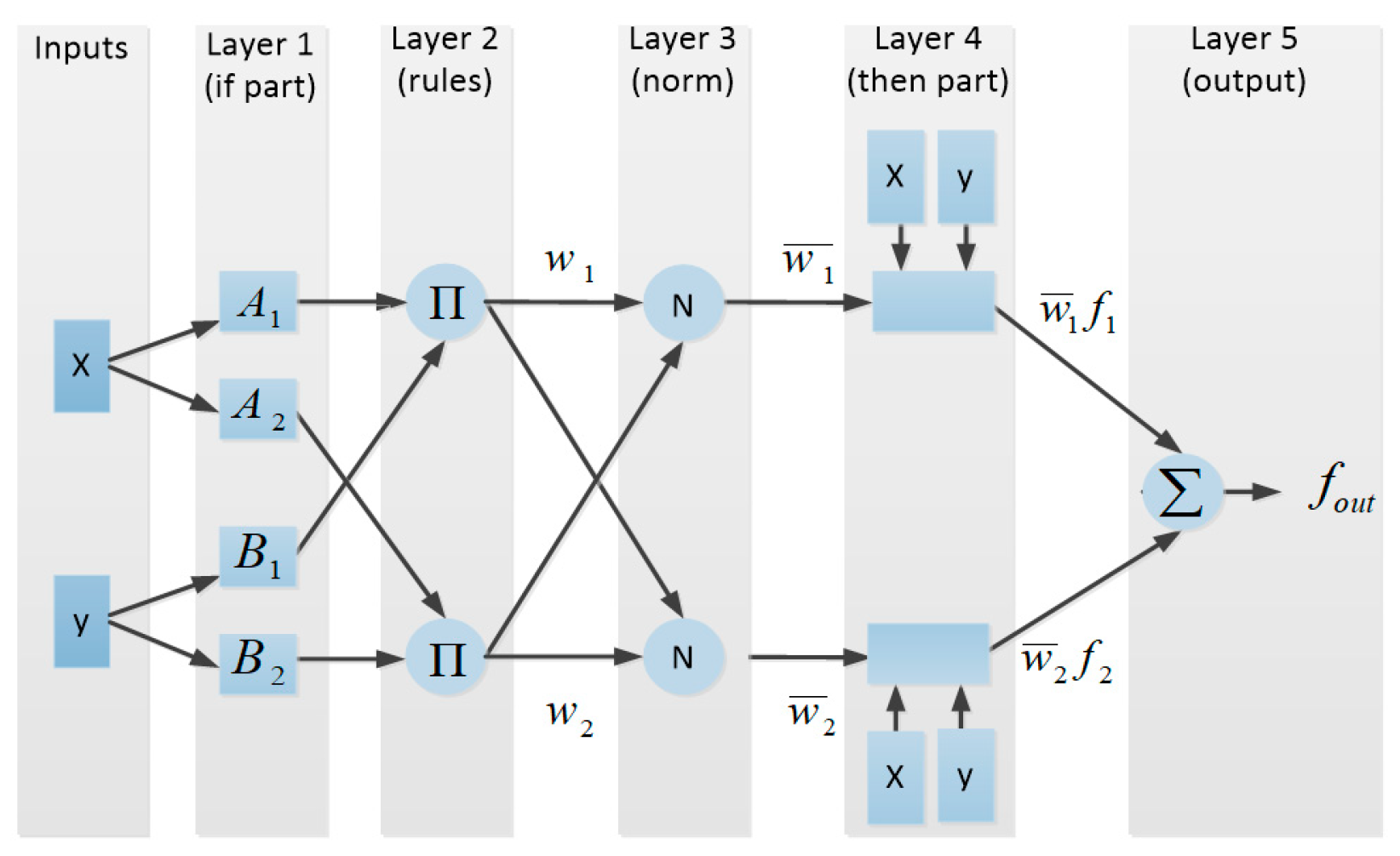
3. Adaptive Neuro-Fuzzy Inference System (ANFIS)

The fuzzy logic method is based on the predetermined “if/then” rules that lack the capability of this system to adapt and learn from new conditions. Thus, to overcome this drawback, authors in [33] hybridized a ANN with a fuzzy inference system (FIS) to form the ANFIS approach. The ANFIS approach is categorized as an enhanced adaptive system like ANN, that, through training, adapts the antecedent (fuzzy membership functions) parameters and the consequent (fuzzy system output function) parameters.
The ANFIS gains the advantages of both ANN and FIS and it does not suffer from the drawbacks associated with both methods. The complicated procedures of ANNs are solved by using linguistic variables of FIS system, and the disadvantage of FIS is bypassed by using the neural inference system, which provides the capability of ANFIS to adapt and learn from new conditions. Therefore, the ANFIS approach has the ability to simulate complex systems using ANN learning with FIS, and it has been classified as a universal estimator capable of predicting the output of complex systems.
ANFIS has been developed as an enhanced adaptive system with group of “if/then” fuzzy rules and tunable membership function (MF) parameters in the training phase. The antecedent (fuzzy membership functions), and the consequent (fuzzy system output function) parameters are two different sets that are optimized during the training phase to provide the learning procedures for ANFIS approach.
ANFIS comprises five different consecutive layers: the first layer is the if-part (fuzzification); the second layer is the rules (production) part; the third layer is norm part; the fourth layer is the then-part (defuzzification); and the fifth layer is the output part [34]. The main ANFIS structure with two inputs (i.e., x and y) as independent variables and one output (i.e., fout) as the dependent variable is illustrated by Figure 1.
Sugeno and Mamdani are two different types of FISs. These two types of FISs have different defuzzification procedures and consequences in “if/then” fuzzy rule sets.
ANFIS architectures represent both the Mamdani and Sugeno methods. In contrast to Sugeno-type FIS, Mamdani has less flexibility to be integrated with the ANFIS approach to precisely model the complex systems [35].
The “if/then” rules of ANFIS approach integrated with first order Sugeno FIS are defined as:
Rule 1:    If x is A1 and y is B1 then z is f1(x, y; p1, q1, r1) = x p1 + y q1 + r1
  Rule 2:    If x is A2 and y is B2 then z is f2(x, y; p2, q2, r2) = x p2 + y q2 + r2
where fi (x, y; pi, qi, ri) is a polynomial function providing the output of fist order Sugeno FIS. In this function, the two inputs of the ANFIS model are represented by x and y, and the output of the ANFIS model is indicated by z. The fuzzy sets are represented by Ai and Bi.
Generally, different node functions constrict the layers of ANFIS approach. As illustrated in Figure 1, the adaptive node, the adjustable variable, is indicated by a square and the fixed node, fixed parameter, is indicated by a circle.
● First layer (if-part):
The first layer consists only of adaptive nodes, as represented by the flowing function:
Q 1 , i =   μ A i ( x ) ,       i = 1 , 2
Q 1 , i =   μ B i 2 ( y ) ,       i = 3 , 4
The inputs to the node i are represented by x and y. Ai and Bi are different linguistic labels. The MF for Ai and Bi fuzzy sets are represented by   μ A i and μ B i , respectively. The membership degree of a fuzzy set is represented by Q1,i. The node i output determines the grade to which each x or y input complies with the quantifiers.
Generally, any form of typical MF can be implemented in ANFIS approach.
The Gaussian membership function is the most widely used MF that is specified as follows:
μ A ( x ; c , σ ) = e 0.5 ( x c σ ) 2
where   σ and c determined the width and center of the Guassian membership function, respectively.
● Second layer (rules):
The second layer consists of only fixed nodes. The products of all connected signals to the node is considered the output of each node in this layer. This layer determines the firing strength for each fuzzy rule via multiplication of incoming signals as follows:
Q 2 , i = w i = μ A i ( x ) μ B i ( y ) ,       i = 1 , 2
where the firing strength for fuzzy rule is represented by output signal of wi.
● Third layer (normalization):
The third layer consists of only fixed nodes. This layer normalizes the firing strength calculated in the second layer, through computing the ratio of the ith firing strength of the fuzzy rule to sum of all the firing strengths of fuzzy rules.
Q 3 , i = w i ¯ = w i w 1 + w 2         i = 1 , 2
where the normalized firing strength of a fuzzy rule as output signal is represented by w ¯ .
● Fourth layer (then part):
In the fourth layer a node function is adaptive with each node i.
Q 4 , i = w i ¯ f i       i = 1 , 2
where the “if/then” fuzzy rules are defined by the following f1 and f2 functions:
Rule1:    If x is A1 and y is B1 then z=f1(x, y; p1, q1, r1)
  Rule2:   If x is A2 and y is B2 then z=f2(x, y; p2, q2, r2)
where the parameter set known as the consequent parameters are represented by ri, qi, and pi.
● Fifth layer (output):
The fifth layer consists of only a single fixed node that calculates the ANFIS output through adding all the arriving signals.
Q 5 , i = f o u t = i w i ¯ f i = i w i f i i w i =   o v e r a l   o u t p u t       i = 1 , 2
The total output of the ANFIS approach is a summation of all consequent signals. Hence, the total output of the ANFIS approach is defended as follows:
f o u t = w 1 ¯ f 1 + w 2 ¯ f 2 = w 1 w 1 + w 2   f 1 + w 2 w 1 + w 2   f 2 = ( w 1 ¯ x ) p 1 + ( w 2 ¯ x ) p 2 + ( w 1 ¯ y ) q 1 + ( w 2 ¯ y ) q 2 + ( w 1 ¯ ) r 1 + ( w 2 ¯ ) r 2
Finally, a hybrid learning algorithm was applied with the ANFIS approach to accurately tune the parameters.

4. Backtracking Search Algorithm (BSA)

BSA, as one of the newly developed metaheuristic optimization algorithms, has relatively simple constriction, but is an efficient algorithm for finding the optimum solutions in non-convex and multimodal optimization problems. Due to the quite simple structure of BSA, it has been applied to solve various engineering optimization problems. During the evaluation of BSA, a trial population was generated through two enhanced crossover and mutation operators. The structures of enhanced mutation and crossover in BSA are extremely different, with the mutation and crossover operators specified in former optimization algorithms, such as differential evolution (DE) and GA. Those two enhanced operators are applied in this algorithm to provide a balance between exploitation of optimal result and exploration of the optimization search space. BSA has efficient exploitation and exploration capabilities because of several effective mechanisms defined in this optimization algorithm to generate a trial population, control the boundaries of optimization search space and adapt the magnitude of the search direction [34].
BSA has only one control parameter and the performance of this optimization in not excessively sensitive to the preliminary value of this parameter. It does not suffer from drawbacks associated with other metaheuristic methods, such as being computationally expensive, being trapped in local optima, having various control parameters, and being overly sensitive to the initial values of these parameters. Additionally, a track of previous generations is stored in memory to share the past experiences for generating a trial population. It stores a randomly chosen population from previous generation in its memory for the generation of the matrix of the search-direction. The superiority of BSA for finding optimum solutions in numerical optimization problems over different widely used metaheuristic optimization algorithms is verified through the statistical analysis reported in [31]. Generally, six different steps construct the BSA structure as coded in Figure S1. The steps of BSA are as follows:
Step 1: Initialization
Scattering the population members in the solution space (Equation (11))
P i , j ; g = 0 ~ U ( l o w j , u p j ) , y i = f ( P i ) f o r i = { 1 , 2 , 3 , , n P o p } , j = { 1 , 2 , 3 , , n V a r }
where:
nPop is population size. nVar signifies the optimization variable. Uniform distribution function is U. lowj and upj are upper and lower search space limits of jth variable. yi is productivity of ith individual. g is generation number.
Step 2: Selection-I
(1)
Initializing a historical population (old P) to determine the search-direction matrix (Equation (12));
(2)
Redefining the historical population at each iteration based on (if/then) rule by comparing two random numbers, a and b. Subsequently, population (P) pursues old P until it is changed to provide a memorization process and facilitates the exploration search space (Equation (13));
(3)
At the end of step 2, a hierarchical sequence has been permuted by shuffling random function (Equation (14));
o l d P i , j ~ U ( l o w j , u p j )
where OldP is a historical population
i f a < b | a , b ~ U ( 0 , 1 ) t h e n o l d P : = P
where, := is the updated operation.
a and b are randomly generated numbers.
o l d P : = p e r m u t i n g ( o l d P )
where,
permuting (oldP) is a random shuffling function.
Step 3: Mutation.
The Wiener process (F) is implemented to control the amplitude of the search matrix according to Equation (15);
M u t a n t = P + F . ( o l d P P ) F = 3 . r n d n | r n d n ~ N ( 0 , 1 )
where,
N is standard normal distribution
Step 4: Crossover.
Determine the binary integer–valued matrix (map) and control parameter of individuals in BSA according to Equation (16);
m a p i , j = 1 ,   i f a < b | a , b ~ U ( 0 , 1 )   t h e n m a p i , u ( 1 : m i x r a t e . r n d . n V a r ) = 0   | r n d ~ U ( 0 , 1 ) , u = p e r m u t i n g ( 1 , 2 , 3 , , n V a r ) e l s e   m a p i , r a n d i ( n V a r ) = 0 T : = M u tan t i f   m a p i , j = 1   t h e n   T i , j : = P i , j f o r i = { 1 , 2 , 3 , , n P o p } , j = { 1 , 2 , 3 , , n V a r }
where mix rate is the control parameter of optimization algorithm.
Step 5: Boundary control.
At the end of step 4, if an individual in generated offspring (T) violates the boundary condition, the control mechanism developed in step 5 is updated according to Equation (17);
i f ( T i , j < l o w j ) o r ( T i , j > u p j ) t h e n T i , j ~ U ( l o w j , u p j )
where,
T is generated offspring
Step 6: Selection-II.
Calculating the fitness and the position (Equation (18)).
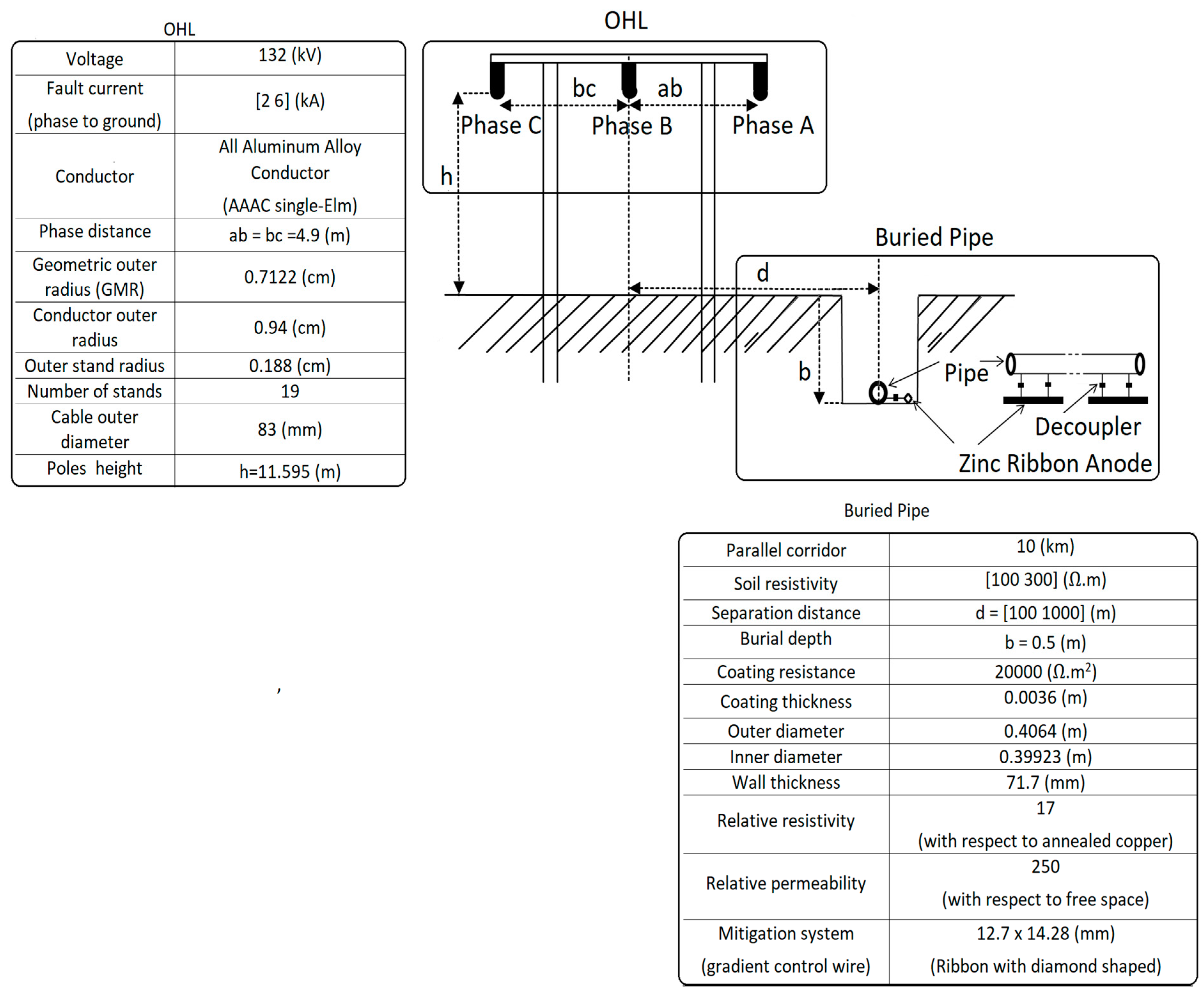
i f   f ( T i ) < y i   t h e n   ,   y i : = f ( T i ) ,   P i : = T i y g = m i n ( f ( P g ) ) i f   y g < y g 1   t h e n   g l o b a l   m i n i m u m : = y g   ,   g l o b a l   m i n i m i z e r : = P g   ,   g = g + 1 f o r i = { 1 , 2 , 3 , , n P o p } , g = { 1 , 2 , 3 , , g M a x }

5. System Modeling

The system modeled in this research is provided in Figure 2. It is comprised of 132 kV OHL and a neighboring, well coated 16″ pipeline. The total length of the metallic pipeline is 10 km, whereas the high voltage OHL length is 20 km. The length of the parallelism of OHL with the pipeline is 10 km; the metallic pipeline is located at the central site with a burial depth of half meter, connected to the gradient control wires as mitigation system. The gradient control wire, as an effective type of mitigation system, is a horizontally-buried zinc anode wire placed at the bottom of the trench beside the metallic pipeline [13], and regularly connected to the metallic pipeline, as illustrated in Figure 2. The gradient control wires typically connect to the pipeline at intervals varying from 150 to 600 m. The DC decoupling devices are connected between the pipeline and gradient control wire, which will decouple the DC while remaining the AC coupled. The function of this device is providing a path for the AC current to flow from the pipeline to the zinc ribbon grounding system, while blocking the DC cathodic protection current from flowing to the zinc ribbon conductor.

6. Simulation Results and Discussion

In this paper, ANFIS-BSA is applied to improve the accuracy of induced voltage prediction on mitigated and unmitigated pipelines. The level of the induced pipelines voltage, depends on diverse factors, such as the level of OHL voltage, parallelism length, the separation distance, resistivity of the ground, the load current magnitude, OHL configuration, and the material of pipeline coating and the mitigation system. The level of fault current, the separation distance, mitigation system, and the resistivity of the ground have the higher impacts on the induced pipeline voltage, as reported in [26]. Generally, the single phase to ground fault condition is considered to evaluate the induced voltage on neighboring pipelines as it is the most frequent fault in the distribution and transmission power system and it produces very high level of induced voltage on the metallic pipelines. This can be explained by the fact that within the two or three phase-to-ground fault occurrences, cancellation of the magnetic field will occur as a result of a poorer induced voltage generated on the metallic pipeline. Hence, in this study, the maximum induced voltage on the pipeline is calculated for mitigated and unmitigated pipelines with varying separation distances, various resistivities of ground, and a diverse level of single line to ground fault currents. The parameters of the system used in this study are tabulated in Figure 2. This data set of input variables covers diverse sets of possible situations.
The validity of the obtained models is verified by comparing the simulation results with the corresponding results obtained from the CDEGS software. Furthermore, to assess the effectiveness of ANFIS-BSA for predicting the induced pipeline voltage, its performances are compared with the following methods: MLP, SVR, ANFIS, MLP-PSO, MLP-CSA, MLP-BSA, SVR-PSO, SVR-CSA, SVR-BSA, ANFIS-PSO, and ANFIS-CSA.
The procedure of the proposed methodology for predicting the induced voltage on both mitigated and unmitigated pipelines is illustrated in Figure 3. Commonly, for finding the practical models generated by the machine learning algorithms, a similar process is carried out. Hence, for obtaining the optimal AI based models to predict the induced voltage on the metallic pipelines, the following serial steps are followed for all applied approaches in this study.
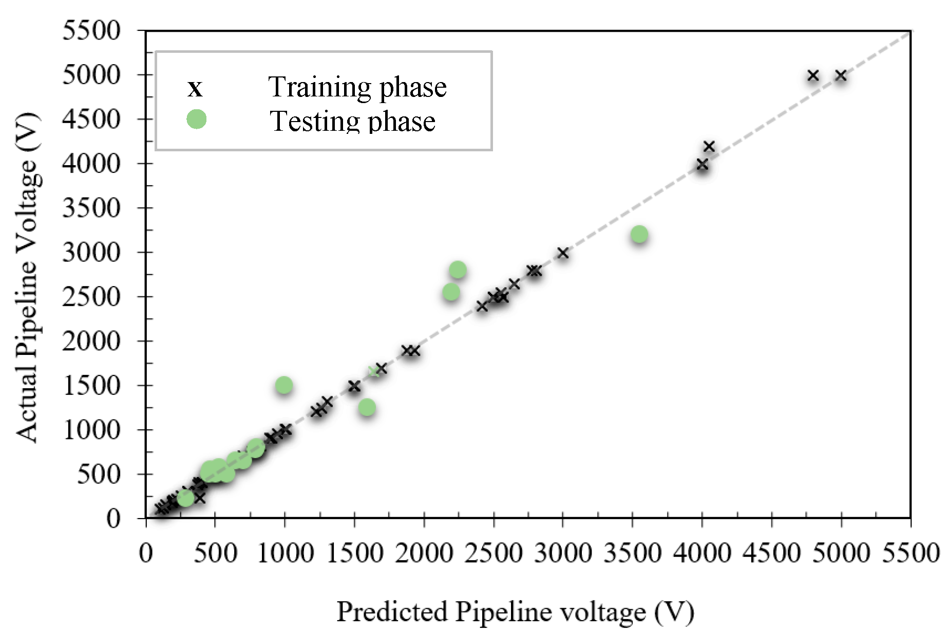
  • The independent variables consisted of four inputs representing fault current, soil resistivity, separation distance, and mitigation system, while the dependent variable represented the total pipeline’s maximum voltage.
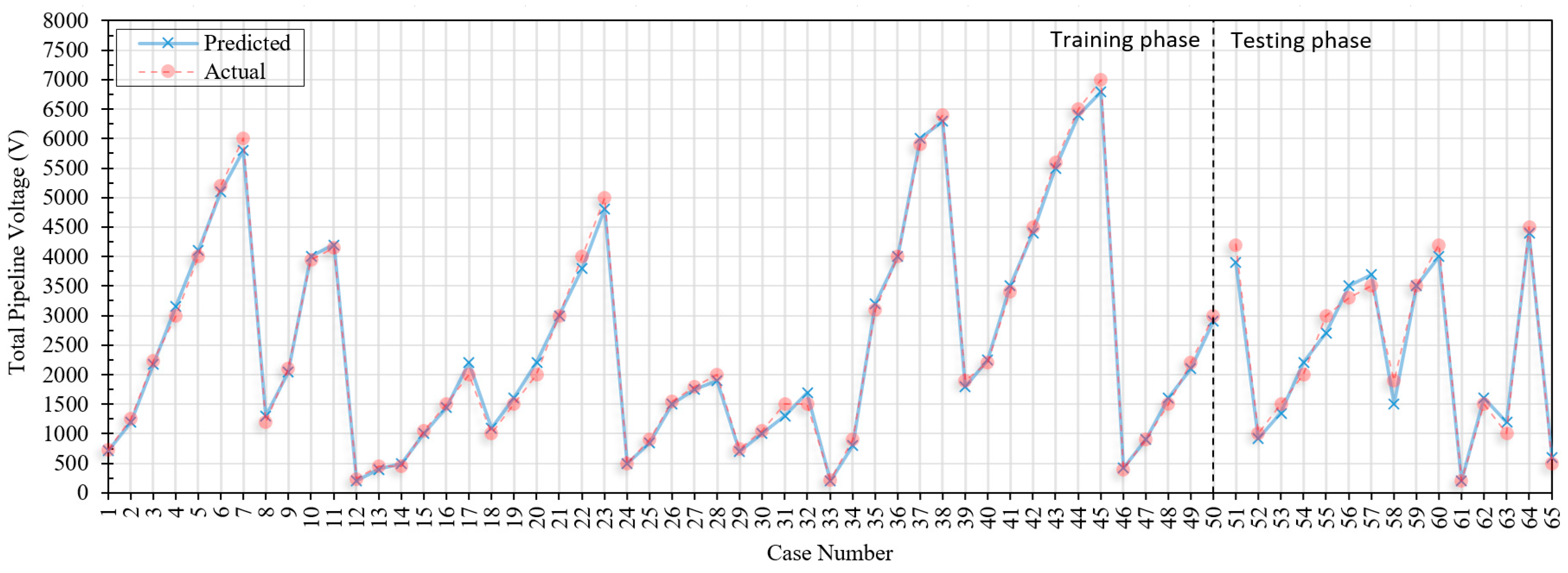
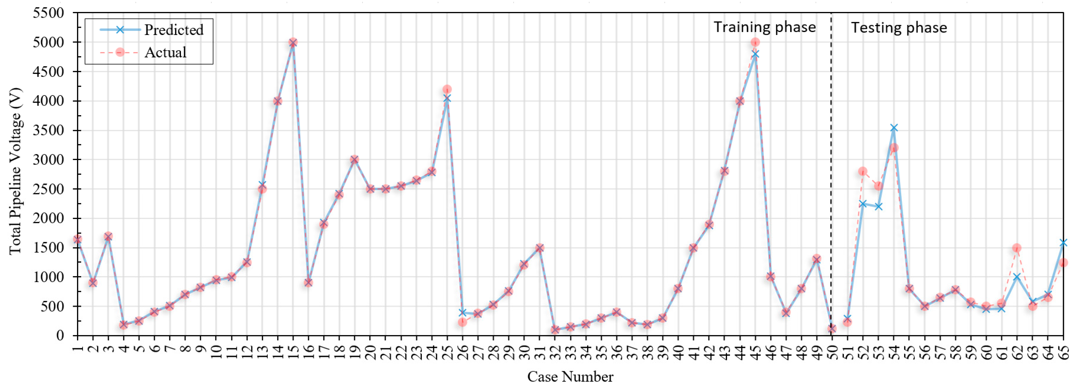
  • Both dependent and independent variables were randomly distributed into two different phases: fifty of the total sixty-five systems with different configurations as the training phase, and the reminder as the testing phase. Since the range of dependent and independent variables varies widely, both variables were normalized by Equation (19). To speed up the learning process, the observed data were normalized prior to data processing. The main purpose of raw data normalization was unifying the observed data into a common scale.
    Z _ _ ( t ) = Z ( t ) min ( Z ) max ( Z ) min ( Z ) + 1
    where Z is the data to be normalized and Z _ _ is the normalized data, and t is the number of observations.
  • The learning process occurred during the training phase. The computer programs that link the input variables to the output were developed during learning process. The data required for the training of the AI-based methods was obtained via the CDEGS program. This program is especially designed to automate and simplify the modeling of complex RoW arrangements involving power transmission lines and other utilities, such as water, oil, or gas pipelines. Its results were strongly validated by analytical equations and by an experimental test rig reported in [8,36].
    Although the testing phase does not have any role in developing the models, it was employed to assess the performance of the models obtained by AI-based methods. To measure the predictive accuracy of the generated models, several evaluation criteria were used, such as Thiel’s inequality coefficient (U-statistic), root mean square error (RMSE), absolute error, and mean absolute percentage error (MAPE). The mathematical equations of those criteria are as follows:
    M A P E % = 1 N t = 1 N | ( E P ( t ) a c t u a l E P ( t ) e s t i m a t e d ) | E P ( t ) a c t u a l × 100
    M A P E % = 1 N t = 1 N | ( E P ( t ) a c t u a l E P ( t ) e s t i m a t e d ) | E P ( t ) a c t u a l × 100
    U = R M S E 1 N t = 1 N ( E P ( t ) a c t u a l ) 2 + 1 N t = 1 N ( E P ( t ) e s t i m a t e d ) 2
    where the U-statistic provides a measure of how well fitted a time series of predicted values to a corresponding time series of observed data. The U-statistic is always in the range of zero to one, with a value closer to one indicating the estimation is no better than a naive estimate and the value closer to zero demonstrates higher prediction accuracy with a great fit.
  • The Durbin–Watson (whiteness) test was calculated to guarantee that the generated models sufficiently describe given data sets [37]. The whiteness test is calculated via a confirmatory analysis. The main purpose of confirmation analysis is to guarantee the whiteness of estimated residuals. The whiteness of estimated residuals (e(t)) indicates that they are uncorrelated. The residuals autocorrelation function (RACF) is used to study the correlation of the whiteness of estimated residuals through the following equation:
    R A C F = | t = 2 N ( e ( t ) e ( t 1 ) ) | t = 1 N ( e ( t ) ) 2
The RACF values come into the range of zero to one; if the value of RACF is meaningfully diverse from zero, it will fall outside a confidence level. This specifies that the residuals are not correlated (white) and an important input (independent) variable has been missed in the tested model.
Since there is no conformity in the optimal values of the machine learning algorithms’ parameters, setting the control parameters of all applied AI-based approaches was done according to the successful approaches in the literature. All parameter settings of applied methods are summarized in Table 1. The optimization methods used the learning process of MLP according to [38] and the optimized SVR approaches were developed based on [39].
The performances of applied machine learning methods for predicting the total induced voltage on unmitigated pipeline are tabulated in Table 2. The RACF values in these tables verify the whiteness of estimated residuals within a confidence interval for all developed models. The prediction accuracy of the studied methods in terms of multi-criteria decisions, using the mean rank of the methods for each indicator (MAPE, U-statistic, absolute error, and RMSE) in whole set is ranked: ANFIS-BSA > ANFIS-CSA > ANFIS-PSO > SVR-BSA > SVR-PSO > SVR-CSA > MLP-BSA > MLP-CSA = ANFIS > MLP-PSO > MLP > SVR.
The comparison between the accuracy of methods applied for the prediction the induced voltage on an unmitigated pipeline reveals that optimized ANFIS approaches outperform other studied methods. Furthermore, it was found that the most efficient optimization algorithm applied for training ANFIS was BSA, as the superior MAPE (1.1581%), U-statistic (0.0072), RMSE (0.0197), and absolute error (1.0213) values reported in Table 2 belong to ANFIS-BSA. The performance of proposed method (ANFIS-BSA) in testing and training phases is depicted in Figure 4 and Figure 5.
For further examination of solution methodology, the performance of optimized ANFIS for predicting the total induced voltage on mitigated pipeline is compared with those from other machine learning methods, as shown in Table 3. The computed RACF values in this table specify that the estimated residuals of all developed models are uncorrelated and attained models satisfactorily describe the given data series.
The prediction accuracy of applied approaches in terms of multi-criteria decisions using the mean rank of methods for each indicator (MAPE, U-statistic, absolute error, and RMSE) in whole data set is ordered: ANFIS-BSA > ANFIS-CSA > ANFIS-PSO > ANFIS = SVR-BSA > SVR-PSO > MLP-BSA > SVR-CSA > MLP-PSO > MLP-CSA > MLP > SVR.
The comparison between accuracy of studied methods for predicting the total induced voltage on mitigated pipeline reveals that optimized ANFIS approaches outperform the other studied methods. The superior MAPE (0.774%), U-statistic (0.01), RMSE (0.0258), and absolute error (1.2037) values reported in Table 3 belong to the ANFIS-BSA model. Thus, it can be determined that the most effective applied optimization algorithm for training ANFIS is BSA. Figure 6 and Figure 7 demonstrate the performance of the ANFIS-BSA method for predicting the total induced voltage on a mitigated pipeline during training of the design phase and testing phase.
Different statistical indexes are applied for further validation of the obtained ANFIS-BSA models. To evaluate the performance of the developed model, the following attributes were recommended [40]:
  • There is a strong correlation between the observed data and the predicted values if the generated model provides 0.8 < | R |.
  • There is a moderate correlation between the observed data and the predicted values if the generated model provides 0.8 > | R | > 0.2.
  • There is a weak correlation between the observed data and the predicted values if the generated model provides 0.2 > | R |.
Table 4 tabulates all the statistical factors of the developed models by ANFI-BSA for predicting the total induced voltage on mitigated and unmitigated pipelines. As shown, the developed models fulfill all the required conditions. The validation phase confirms that proposed method (ANFIS-BSA) generates accurate models, which is strongly applicable for predicting the total induced voltage on mitigated and unmitigated pipelines.
Furthermore, from the connections of the generated ANN models it can be found that separation distances, mitigation effect, soil resistivity, and the phase current’s magnitude have the highest contributions to the induced pipeline voltage levels, respectively. As the separation distance between OHL and pipeline RoW is the most influential parameter on the magnitude of induced voltage, it should be determined prudently to keep the pipelines at safe distances from OHLs. It also indicates that a mitigation system presents significant influence on the level of pipeline voltage. Thus, the developed ANSIS-BSA method was applied to predict the mitigated and unmitigated pipeline voltages at different fault currents and soil resistivities for a wide range of separation distances. Additionally, to validate the reliably of the proposed method, its estimates are compared with those observed from CDEGS program. The comparison between the observed and predicted total pipeline voltages at different soil resistivities and fault currents for a range of separation distances, with and without a mitigation system, are illustrated in Figure 8. According to the simulation results it was found that there is an adequate agreement between the ANFIS-BSA predictions and the observed data. The simulation results clearly indicate that by increasing the separation distances the strength of the electromagnetic field will be reduced; consequently, the pipeline’s voltage level will be decreased. It also can be seen that in the small separation between the OHL and the pipeline, the effect of fault current on the total pipeline potential is more severe than the effect of soil resistivity. Moreover, the obtained results confirmed that mitigation systems can be used in order to significantly reduce the induced pipeline voltage to acceptable level for various fault conditions.

7. Conclusions

In this work, a hybrid approach composed of ANFIS and BSA has been developed for predicting the voltage on mitigated and unmitigated metallic pipelines built in OHLs’ right-of-way. The actual parameters of the system, the mitigation system, fault current, resistivity of the ground, and separation distance, are taken as the inputs (independent variables) and the pipeline voltages predicted are the output (dependent variable). Regardless of which practical system is investigated, the obtained results indicated that the developed models by ANFIS-BSA provide enhanced estimations over other solutions from AI-based methodologies. Total induced voltage on the pipeline has been modeled by ANFIS, SVR, ANN, and an optimized version of these approaches. According to the obtained results, the ANFIS-BSA models consistently give superior predictions to other studied AI-based methods.
Excellent agreement between obtained data from CDGES program and ANFIS optimized by BSA has been obtained. The relative importance of the independent variables has been also studied. This paper clearly specified the potential of the applied methodology for capturing the interactions between the levels of pipeline voltage and the independent variables, and even for the investigation of the relative importance of these input variables. Additionally, the results demonstrate that developed approach can accurately predict the total pipeline voltage for a wide range of input variables, with and without a mitigation system. The accuracy of the predicted pipeline potential is important for designing mitigation systems that will increase the overall pipeline integrity and safety. The developed methodology can be plainly applied for diverse environmental, dimensional, and power system conditions.

Supplementary Materials

The following are available online at https://www.mdpi.com/1996-1073/12/19/3651/s1, Figure S1: Pseudocode of BSA.

Author Contributions

Conceptualization, S.H.A.K., A.A.H. and A.H.A.-B.; methodology, S.H.A.K.; software, S.H.A.K., A.A.H. and A.H.A.-B.; validation, S.H.A.K. and A.H.A.-B.; formal analysis, S.H.A.K.; resources, Y.C.; data curation, A.A.S.; writing—original draft preparation, S.H.A.K.; writing—review and editing, S.H.A.K., A.A.H., and A.H.A.-B.; visualization, Y.C.; supervision, A.A.H., A.H.A.-B. and Y.C.; project administration, A.A.H.; funding acquisition, A.A.S.

Funding

This research was funded by Sultan Qaboos University (SQU) and Petroleum Development Oman (PDO) through Ejaad, under grant number CR/DVC/SERC/18/01.

Conflicts of Interest

The authors declare no conflict of interest. The funders had no role in the design of the study; in the collection, analyses, or interpretation of data; in the writing of the manuscript, or in the decision to publish the results.

References

  1. Czumbil, L.; Micu, D.; Ceclan, A. Artificial Intelligence Techniques Applied to Electromagnetic Interference Problems. In Proceedings of the International Conference on Advancements of Medicine and Health Care through Technology, Cluj-Napoca, Romania, 23–26 September 2009; pp. 339–344. [Google Scholar]
  2. Antunes, C.L.; Micu, D.D.; Czumbil, L.; Christoforidis, G.C.; Ceclan, A.; Şteţ, D. Evaluation of induced AC voltages in underground metallic pipeline. COMPEL Int. J. Comput. Math. Electr. Electron. Eng. 2012, 31, 1133–1143. [Google Scholar]
  3. Ismail, H.M. Effect of oil pipelines existing in an HVTL corridor on the electric-field distribution. IEEE Trans. Power Deliv. 2007, 22, 2466–2472. [Google Scholar] [CrossRef]
  4. Lucca, G. Different approaches in calculating AC inductive interference from power lines on pipelines. IET Sci. Meas. Technol. 2018, 12, 802–806. [Google Scholar] [CrossRef]
  5. Lu, M.; Zhu, W.; Yin, L.; Peyton, A.J.; Yin, W.; Qu, Z. Reducing the lift-off effect on permeability measurement for magnetic plates from multifrequency induction data. IEEE Trans. Instrum. Meas. 2017, 67, 167–174. [Google Scholar] [CrossRef]
  6. Qi, L.; Yuan, H.; Li, L.; Cui, X. Calculation of interference voltage on the nearby underground metal pipeline due to the grounding fault on overhead transmission lines. IEEE Trans. Electromagn. Compat. 2013, 55, 965–974. [Google Scholar] [CrossRef]
  7. Micu, D.D.; Christoforidis, G.C.; Czumbil, L. AC interference on pipelines due to double circuit power lines: A detailed study. Electr. Power Syst. Res. 2013, 103, 1–8. [Google Scholar] [CrossRef]
  8. Al-Badi, A.; Al-Rizzo, H. Simulation of electromagnetic coupling on pipelines close to overhead transmission lines: A parametric study. J. Commun. Softw. Syst. 2005, 1. [Google Scholar] [CrossRef]
  9. Lu, M.; Xie, Y.; Zhu, W.; Peyton, A.J.; Yin, W. Determination of the magnetic permeability, electrical conductivity, and thickness of ferrite metallic plates using a multi-frequency electromagnetic sensing system. IEEE Trans. Ind. Inform. 2018, 15, 4111–4119. [Google Scholar] [CrossRef]
  10. Charalambous, C.A.; Demetriou, A.; Lazari, A.L.; Nikolaidis, A.I. Effects of Electromagnetic Interference on Underground Pipelines caused by the Operation of High Voltage AC Traction Systems: The Impact of Harmonics. IEEE Trans. Power Deliv. 2018, 33, 2664–2672. [Google Scholar] [CrossRef]
  11. Guo, Y.B.; Liu, C.; Wang, D.G.; Liu, S.H. Effects of alternating current interference on corrosion of X60 pipeline steel. Pet. Sci. 2015, 12, 316–324. [Google Scholar] [CrossRef] [Green Version]
  12. Yu, Z.; Liu, L.; Wang, Z.; Li, M.; Wang, X. Evaluation of the Interference Effects of HVDC Grounding Current on a Buried Pipeline. IEEE Trans. Appl. Supercond. 2019, 29, 1–5. [Google Scholar] [CrossRef]
  13. Southey, R.; Dawalibi, F.; Vukonich, W. Recent advances in the mitigation of AC voltages occurring in pipelines located close to electric transmission lines. IEEE Trans. Power Deliv. 1994, 9, 1090–1097. [Google Scholar] [CrossRef]
  14. Djekidel, R.; Bessedik, S.A.; Spiteri, P.; Mahi, D. Passive mitigation for magnetic coupling between HV power line and aerial pipeline using PSO algorithms optimization. Electr. Power Syst. Res. 2018, 165, 18–26. [Google Scholar] [CrossRef] [Green Version]
  15. Youwen, J.; Wuxi, B.; Kaizhi, C.; Meng, L.; Jun, Z. Mitigating Pipeline AC Interference Using Numerical Modeling and Continuous AC Voltage Monitoring. In Proceedings of the CORROSION 2018, Phoenix, AZ, USA, 15–19 April 2018. [Google Scholar]
  16. Popoli, A.; Sandrolini, L.; Cristofolini, A. A quasi-3D approach for the assessment of induced AC interference on buried metallic pipelines. Int. J. Electr. Power Energy Syst. 2019, 106, 538–545. [Google Scholar] [CrossRef]
  17. Czumbil, L.; Micu, D.D.; Stet, D.; Ceclan, A. A neural network approach for the inductive coupling between overhead power lines and nearby metallic pipelines. In Proceedings of the 2016 International Symposium on Fundamentals of Electrical Engineering (ISFEE), Bucharest, Romania, 30 June–2 July 2016; pp. 1–6. [Google Scholar]
  18. Micu, D.D.; Lingvay, I.; Lingvay, C.; Cret, L.; Simion, E. Numerical evaluation of induced voltages in the metallic underground pipelines. Rev. Roum. Sci. Tech. Ser. Electrotech. Energetique 2009, 54, 175–183. [Google Scholar]
  19. Milešević, B. Electromagnetic Influence of Electric Railway System on Metallic Structures; Fakultet elektrotehnike i računarstva, Sveučilište u Zagrebu: Zagreb, Croatia, 2014. [Google Scholar]
  20. Micu, D.D.; Czumbil, L.; Christoforidis, G.; Ceclan, A. Layer recurrent neural network solution for an electromagnetic interference problem. IEEE Trans. Magn. 2011, 47, 1410–1413. [Google Scholar] [CrossRef]
  21. Pourdaryaei, A.; Mokhlis, H.; Illias, H.A.; Kaboli, S.H.A.; Ahmad, S. Short-Term Electricity Price Forecasting via Hybrid Backtracking Search Algorithm and ANFIS Approach. IEEE Access 2019, 7, 77674–77691. [Google Scholar] [CrossRef]
  22. Micu, D.D.; Czumbil, L.; Christoforidis, G.; Simion, E. Neural networks applied in electromagnetic interference problems. Rev. Roum. Sci. Tech. Ser. Electrotech. Energetique 2012, 57, 162–171. [Google Scholar]
  23. Czumbil, L.; Micu, D.D.; Şteţ, D.; Ceclan, A. INDUCTIVE COUPLING BETWEEN OVERHEAD POWER LINES AND NEARBY METALLIC PIPELINES. A NEURAL NETWORK APPROACH. Carpathian J. Electr. Eng. 2015, 9, 29–43. [Google Scholar]
  24. Al-Badi, A.; Ellithy, K.; Al-Alawi, S. Prediction of Voltages on Mitigated Pipelines Paralleling Electric Transmission Lines Using an Arificial Neural Network. J. Corros. Sci. Eng. 2007, 10, 24–28. [Google Scholar]
  25. Al-Badi, A.; Ellithy, K.; Al-Alawi, S. Prediction of Voltages on Mitigated Pipelines Paralleling Electric Transmission Lines Using Ann. Int. J. Comput. Appl. 2010, 32, 15–22. [Google Scholar]
  26. Al-Badi, A.; Ghania, S.M.; El-Saadany, E.F. Prediction of metallic conductor voltage owing to electromagnetic coupling using neuro fuzzy modeling. IEEE Trans. Power Deliv. 2008, 24, 319–327. [Google Scholar] [CrossRef]
  27. Satsios, K.J.; Labridis, D.P.; Dokopoulos, P.S. An artificial intelligence system for a complex electromagnetic field problem. II. Method implementation and performance analysis. IEEE Trans. Magn. 2000, 35, 523–527. [Google Scholar] [CrossRef]
  28. Ghelardoni, L.; Ghio, A.; Anguita, D. Energy load forecasting using empirical mode decomposition and support vector regression. IEEE Trans. Smart Grid 2013, 4, 549–556. [Google Scholar] [CrossRef]
  29. Kaboli, S.H.A.; Fallahpour, A.; Selvaraj, J.; Rahim, N. Long-term electrical energy consumption formulating and forecasting via optimized gene expression programming. Energy 2017, 126, 144–164. [Google Scholar] [CrossRef]
  30. Damousis, I.G.; Satsios, K.; Labridis, D.; Dokopoulos, P. Combined fuzzy logic and genetic algorithm techniques—Application to an electromagnetic field problem. Fuzzy Sets Syst. 2002, 129, 371–386. [Google Scholar] [CrossRef]
  31. Civicioglu, P. Backtracking search optimization algorithm for numerical optimization problems. Appl. Math. Comput. 2013, 219, 8121–8144. [Google Scholar] [CrossRef]
  32. Lee, C.H.; Chang, C.N.; Jiang, J.A. Evaluation of ground potential rises in a commercial building during a direct lightning stroke using CDEGS. IEEE Trans. Ind. Appl. 2015, 51, 4882–4888. [Google Scholar] [CrossRef]
  33. Jang, J.S. ANFIS: Adaptive-network-based fuzzy inference system. IEEE Trans. Syst. Man Cybern. 1993, 23, 665–685. [Google Scholar] [CrossRef]
  34. Abbasi, M.R.; Shamiri, A.; Hussain, M.A.; Kaboli, S.H.A. Dynamic process modeling and hybrid intelligent control of ethylene copolymerization in gas phase catalytic fluidized bed reactors. J. Chem. Technol. Biotechnol. 2019, 94, 2433–2451. [Google Scholar] [CrossRef]
  35. Svalina, I.; Galzina, V.; Lujić, R.; ŠImunović, G. An adaptive network-based fuzzy inference system (ANFIS) for the forecasting: The case of close price indices. Expert Syst. Appl. 2013, 40, 6055–6063. [Google Scholar] [CrossRef]
  36. Al-Badi, A.; Metwally, I. Induced voltages on pipelines installed in corridors of AC power lines. Electr. Power Compon. Syst. 2006, 34, 671–679. [Google Scholar] [CrossRef]
  37. AlRashidi, M.; El-Naggar, K. Long term electric load forecasting based on particle swarm optimization. Appl. Energy 2010, 87, 320–326. [Google Scholar] [CrossRef]
  38. Le, L.T.; Nguyen, H.; Dou, J.; Zhou, J. A Comparative Study of PSO-ANN, GA-ANN, ICA-ANN, and ABC-ANN in Estimating the Heating Load of Buildings’ Energy Efficiency for Smart City Planning. Appl. Sci. 2019, 9, 2630. [Google Scholar] [CrossRef]
  39. Bessedik, S.A.; Djekidel, R.; Ameur, A. Performance of different kernel functions for LS-SVM-GWO to estimate flashover voltage of polluted insulators. IET Sci. Meas. Technol. 2018, 12, 739–745. [Google Scholar] [CrossRef]
  40. Mostafavi, E.S.; Mousavi, S.M.; Hosseinpour, F. Gene Expression Programming as a Basis for New Generation of Electricity Demand Prediction Models. Comput. Ind. Eng. 2014, 74, 120–128. [Google Scholar]
Figure 1. Overall configuration of the adaptive neuro-fuzzy inference system (ANFIS).
Energies 12 03651 g001
Figure 2. Cross section of 132-kV overhead lines (OHL) and the buried pipeline with a mitigation system.
Energies 12 03651 g002
Figure 3. Procedure of ANFIS-BSA for induced pipeline voltage prediction.
Energies 12 03651 g003
Figure 4. Performance of proposed method (ANFIS-BSA) during testing and training phases for predicting the total induced voltage on unmitigated pipeline.
Energies 12 03651 g004
Figure 5. Actual versus predicted results of ANFIS-BSA for unmitigated pipeline.
Energies 12 03651 g005
Figure 6. Performance of the proposed method (ANFIS-BSA), during testing and training phases, for prediction of the total induced voltage on mitigated pipeline.
Energies 12 03651 g006
Figure 7. Actual versus predicted results of ANFIS-BSA for mitigated pipeline.
Energies 12 03651 g007
Figure 8. Total pipeline voltages at different fault current and soil resistivities. (a) 4 kA at 300 Ω.m without mitigation system. (b) 2kA at 100 Ω.m without mitigation system. (c) 4 kA at 300 Ω.m with mitigation system. (d) 2kA at 100 Ω.m with mitigation system.
Energies 12 03651 g008
Table 1. Parameter settings of applied methods.
MethodsParametersValue
ANNMLPHidden layer
Transfer function
Learning algorithm
1
logarithmic sigmoid
Levenberg-Marquardt PB
SVRRBF kernelKernel’s parameter (∂)
Soft margin parameter (C)
Fraction of error (ʋ)
1/6
1
0.5
ANFISSubtractive clustering (SC)Cluster radius0.8
FIS structureSugeno-type
Membership functionGaussian
Metaheuristic optimizationPSOSwarm population
w
c1=c2
100
[0.4, 0.9]
2
CSANumber of nests
Distribution factor (ß)
Probability of an alien egg (Pa)
100
1.5
[0, 1]
BSANumber of individuals100
Control parameter rate (P)100%
Table 2. Comparison between the accuracy of the applied approached for predicting the total induced voltage on an unmitigated pipeline.
MethodsPerformance IndexesMAPE (%)RMSEAbsolute ErrorU-StatisticRACF
MLPTraining1.28360.03650.93280.00910.0007
Testing1.96270.05590.74320.01540.0003
Whole set1.50170.04621.67600.01100.0006
MLP-PSOTraining1.23770.03430.91720.00880.0004
Testing1.89740.05320.72320.01520.0022
Whole set1.45340.04351.64040.01060.0014
MLP-CSATraining1.20340.03140.89730.00870.0043
Testing1.88790.05220.71890.01500.0019
Whole set1.41790.03991.61620.01040.0035
MLP-BSATraining1.18350.28450.88750.00860.0008
Testing1.86610.50430.69590.01490.0035
Whole set1.39790.03771.58340.01020.0021
SVRTraining1.30450.03970.95200.00970.0032
Testing1.99030.05990.77360.01580.0045
Whole set1.62730.04831.72560.01140.0038
SVR-PSOTraining1.11940.02640.86140.00840.0035
Testing1.72870.04710.65670.01510.0007
Whole set1.35860.03521.51810.00980.0025
SVR-CSATraining1.12080.02730.87060.00850.0017
Testing1.73220.04860.66130.01470.0013
Whole set1.36270.03671.53190.01010.0016
SVR-BSATraining1.11740.02530.85060.00810.0009
Testing1.72480.04580.64230.01400.0074
Whole set1.35410.03351.49290.00950.0028
ANFISTraining1.21580.03290.90030.00860.0008
Testing1.88450.05180.71150.01490.0011
Whole set1.42340.04061.61180.01030.0009
ANFIS-PSOTraining0.99120.02490.80100.00740.0024
Testing1.64320.04050.60230.01310.0028
Whole set1.21050.02791.40330.00810.0019
ANFIS-CSATraining0.98680.02070.74120.00650.0004
Testing1.62470.03220.57080.01140.0011
Whole set1.19400.02551.31200.00780.0010
ANFIS-BSATraining0.96840.01600.60070.00580.0012
Testing1.58490.02610.42060.01000.0017
Whole set1.15810.01971.02130.00720.0015
Table 3. Comparison between the accuracy of the applied approached for predicting the total induced voltage on a mitigated pipeline.
MethodsPerformance IndexesMAPE (%)RMSEAbsolute ErrorU-StatisticRACF
MLPTraining0.74510.02271.78450.00970.0002
Testing2.41010.15411.47120.03100.0005
Whole set1.11250.04783.25570.01890.0004
MLP-PSOTraining0.65210.02011.59240.00880.0017
Testing2.22730.12871.28730.02510.0022
Whole set0.95470.04212.87980.01570.0020
MLP-CSATraining0.70170.02181.67380.00930.0004
Testing2.34140.13241.36710.02750.0002
Whole set1.09870.04413.04090.01700.0003
MLP-BSATraining0.60130.01931.50240.00800.0032
Testing2.20140.12141.20170.02230.0006
Whole set0.91010.04002.70410.01250.0019
SVRTraining1.23490.03322.21450.01280.0032
Testing2.74970.17622.00110.03980.0045
Whole set1.57430.06244.21560.02960.0038
SVR-PSOTraining0.59780.01861.47860.00760.0040
Testing2.17850.12041.19630.02170.0021
Whole set0.90020.03872.67490.01180.0028
SVR-CSATraining0.62130.01951.52070.00850.0015
Testing2.23140.12251.22030.02320.0016
Whole set0.92300.04212.70410.01370.0015
SVR-BSATraining0.57230.01781.41220.00710.0014
Testing2.09940.11921.18010.02020.0018
Whole set0.88790.03712.59230.01050.0015
ANFISTraining0.35340.01280.77890.00490.0021
Testing1.98760.05600.58230.02070.0003
Whole set0.86340.03431.36120.01160.0013
ANFIS-PSOTraining0.31340.01200.75670.00420.0009
Testing1.93920.05320.56680.01980.0013
Whole set0.80830.03271.32350.01110.0012
ANFIS-CSATraining0.30340.01090.73870.00390.0007
Testing1.92330.05030.55230.01930.0002
Whole set0.79540.03101.29100.01050.0005
ANFIS-BSATraining0.27300.00950.68900.00360.0014
Testing1.90110.04420.51470.01840.0010
Whole set0.77400.02581.20370.01000.0011
Table 4. Statistical factors of the ANFIS-BSA models for predicting the total induced voltage on mitigated and unmitigated pipeline.
ItemFormulaConditionANFIS-BSA
Unmitigated
ANFIS-BSA
Mitigated
1R0.8 < R00.99970.9965
2 K = | i = 1 n ( h i × t i ) | i = 1 n h i 2 0.85 < k < 1.150.99750.9993
3 K = | i = 1 n ( h i × t i ) | i = 1 n t i 2 0.85 < k’ < 1.151.00141.0017
4 m = R 2 R 0 2 R 2 │m│ < 0.1−0.0024−0.0014
5 n = R 2 R 0 2 R 2 │n│ < 0.1−0.0013−0.0033
6 R m = R 2 × ( 1 | R 2 R 0 2 | ) 0.5 < Rm0.99810.9923
Where R 0 2 = 1 i = 1 n ( h i t i 0 ) 2 i = 1 n ( t i t i ) 2 , h i 0 = k × t i 0.8 < R02 < 11.00001.0000
R 0 2 = 1 i = 1 n ( h i t i 0 ) 2 i = 1 n ( h i h i ) 2 , t i 0 = K × t i 0.8 < R0’ 2 < 11.00001.0000

