Building Energy Performance Analysis: An Experimental Validation of an In-House Dynamic Simulation Tool through a Real Test Room


Abstract
:
1. Introduction
1.1. Literature Review
1.2. Aim of the Work and Content of the Paper
- a flexible tool to be used for the implementation of new add-on models able to suitably assess the energy performance of future building research challenges (e.g., innovative envelope integrated technologies and strategies, new energy efficiency construction materials, real users’ interaction with the building indoor environmental control systems, innovative building plants, etc.) [48,70,71].
- Finally, as DETECt successfully surpassed the validation process, which intrinsically suggests the consistency of the developed models in properly predicting the indoor space thermal behavior, a novel case study analysis developed through DETECt is presented here. Specifically, the use of solar radiation reflective coatings and low-emissivity plasters for building opaque elements is investigated. It is worth noting that such innovative passive envelope solutions [80,81,82] are gaining much more interest as they can be easily implemented in new or existing buildings in order to reduce their energy consumption [83]. Nevertheless, the available literature on these materials (e.g., references [84,85,86,87,88,89]) highlights that much research work is needed, because of the following:
- Commercial software often does not allow variable optical properties of the envelope surfaces (e.g., solar reflectance) to be setup, or to take into account the effective spectral distribution of the incident solar radiation (e.g., [90]).
2. Model Description
2.1. Description of the Framework and General Consideration
2.2. Heat Flow Calculation Procedure
3. Model Validation
3.1. Empirical Validation Procedure
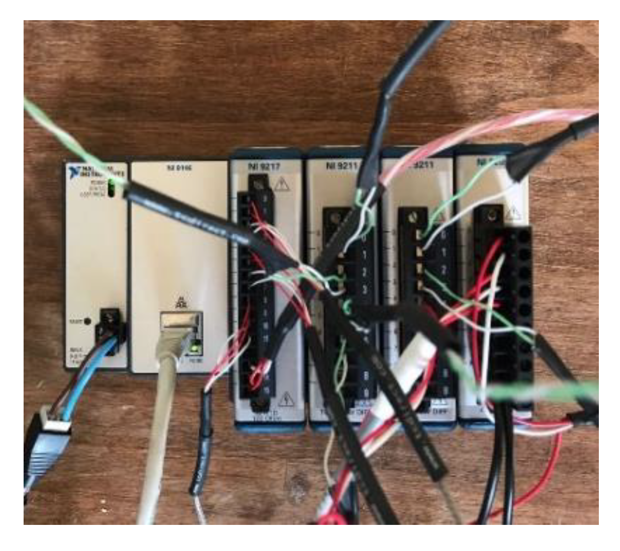
3.1.1. Experimental Set-Up
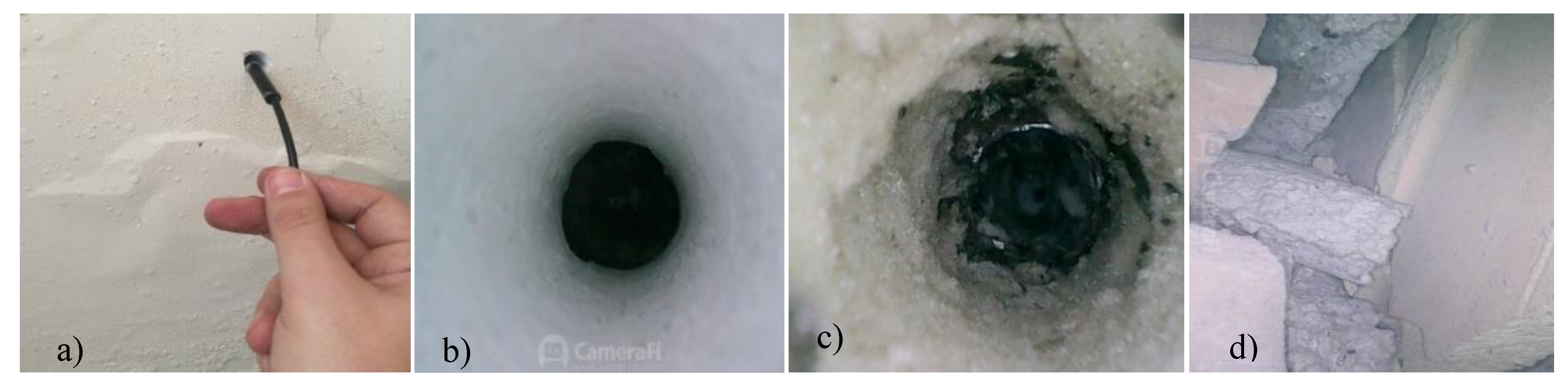
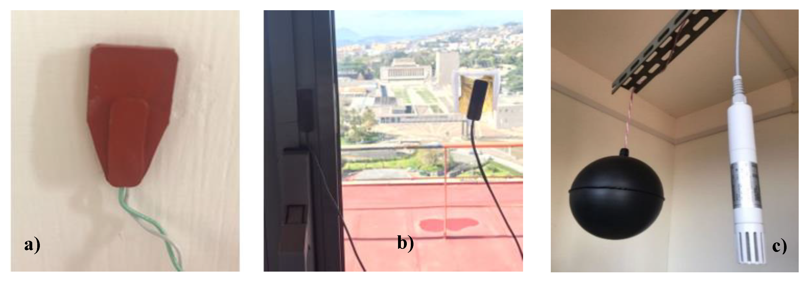
- Six thermocouples for measuring the internal surfaces temperature of the North-West, North-East, South-East, South-West walls, ceiling and floor (K-type, model TC Direct 402–805. Measuring range: from −250 to 150 °C. Accuracy: ± 1.0 °C or ±0.75%). See Figure 5a. Note that, the temperature homogeneity on the surfaces of such test room elements was repeatedly verified by means of an infrared thermo-camera (FLIR, model T335. Measuring range: from –20 to 650 °C; in 3 ranges: −20 to 120 °C or 0 to 350 °C or 200 to 650 °C. Accuracy: ±2 °C or 2%. Thermal sensitivity/NETD 50 mK at 30 °C. IR resolution: 320 × 240 pixels).
- Three thermoresistances for measuring the temperature of internal surfaces of the door and of window glass and frame (PT 100, model TC Direct 515–680. Measuring range: from −50 to 150 °C. Accuracy: ± 0.3 °C at 0 °C). See Figure 5b.
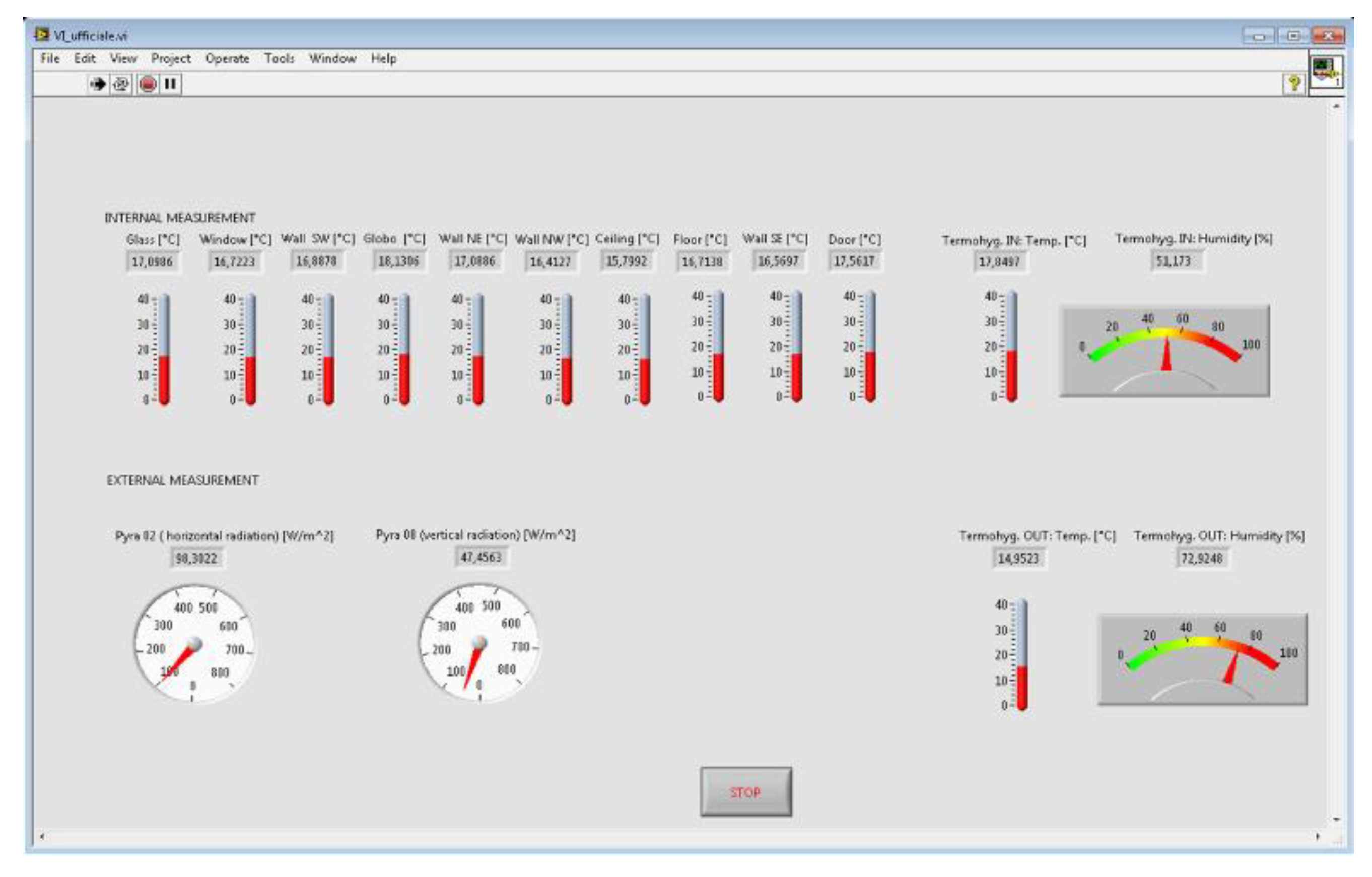
- One hygro-thermometer for measuring the indoor air temperature and humidity (HD 9008 TRR. Platinum resistance thermometer, 100 Ω. 4–20 mA output, and 10–30 VDC power supply. Temperature measuring range: −40 to 80 °C. Accuracy: ± 0.15 °C or ± 0.1%. Hygroscopic polymer humidity sensor. 4–20 mA output. Relative humidity measuring range: from 0 to 100%. Accuracy: ± 1.5% in the range 0%–90% and ± 2.0% elsewhere. See Figure 5c, right.
- One globe-thermometer for measuring the mean radiant temperature of the test room indoor surfaces, with an inside thermocouple (K-type, model TC Direct 402–805. Measuring range: from −250 to 150 °C. Accuracy: ± 1.0 °C or ± 0.75%). See Figure 5c, left.
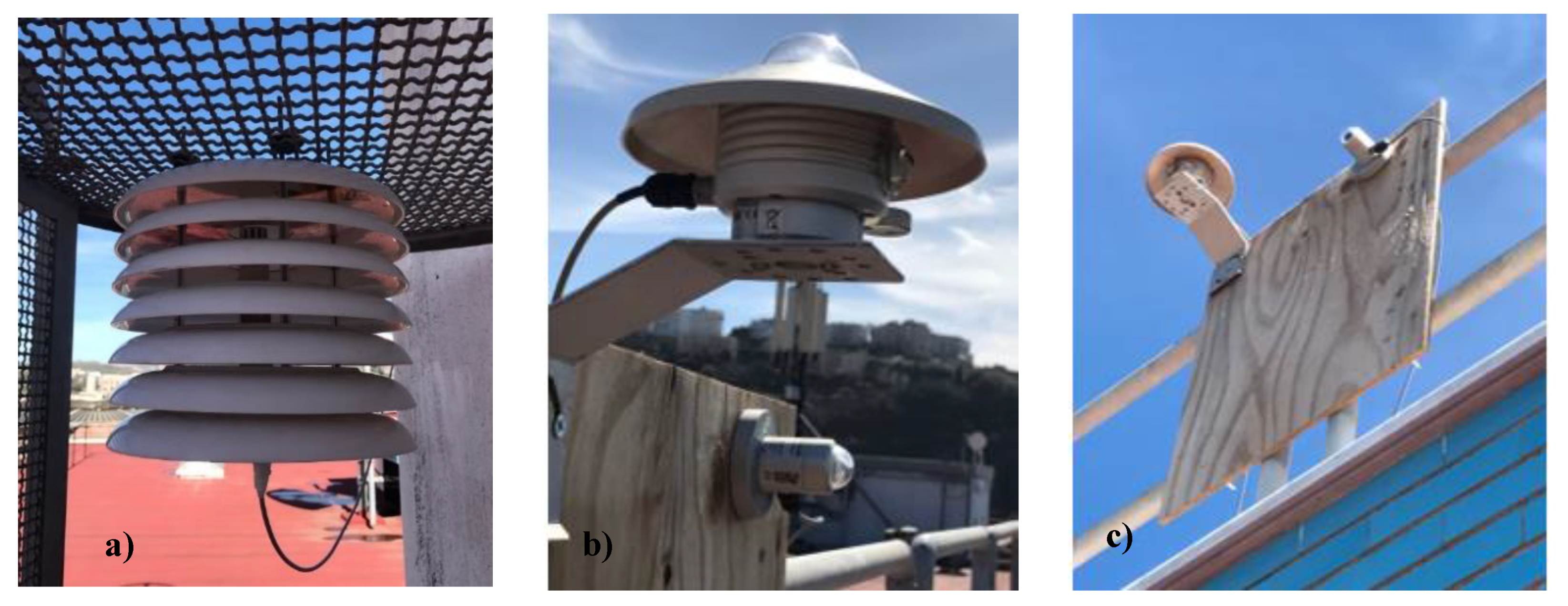
- One hygro-thermometer for measuring the outdoor air temperature and humidity (HD 9008 TRR, above described), protected by a multi-plate radiation shield. See Figure 6a.
- One pyranometer for measuring the horizontal global incident solar radiation (Delta Ohm, LP Pyra 02 AC. First Class pyranometer based on a thermopile sensor. 4–20 mA output. Measuring range: 0–2000 W/m2. Operating temperature range: −40–80 °C. Sensitivity: 10 µV/W/m2. Impedance: 33–45 Ω. Device protected by two concentric domes. See Figure 6b,c;
- One pyranometer for measuring the vertical South-West global incident solar radiation (Delta Ohm, LP Pyra 08 BL. Second Class pyranometer. 4–20 mA output. Measuring range: 0–2000 W/m2. Operating temperature range: −40 to 80 °C. Sensitivity: 15 mV/kW/m2. Impedance: 5 Ω. Device protected by two concentric domes. Figure 6b,c.
- Two hygro-thermometers for measuring the temperature and humidity boundary conditions external to the test cell. One placed in the corridor of the twelfth floor (linked to the South-West tests room wall), and the other one at the eleventh floor of the building, in the floor adjacent space to the test room (Testo 174H. 2-channel temperature and humidity mini data logger for continuous building climate monitoring. Temperature measuring range: from −20 to +70 °C. Accuracy: ± 0.5 °C. Resolution: 0.1 °C. Relative humidity measuring range: from 2% to 98%. Accuracy ± 3%. Resolution: 0.1%).
3.1.2. Experimental Analysis
- from March 23rd at 12:00 am to March 29th at 11:59 pm (winter climate time);
- from July 1st at 12:00 am to July 7th at 11:59 pm (summer climate time);
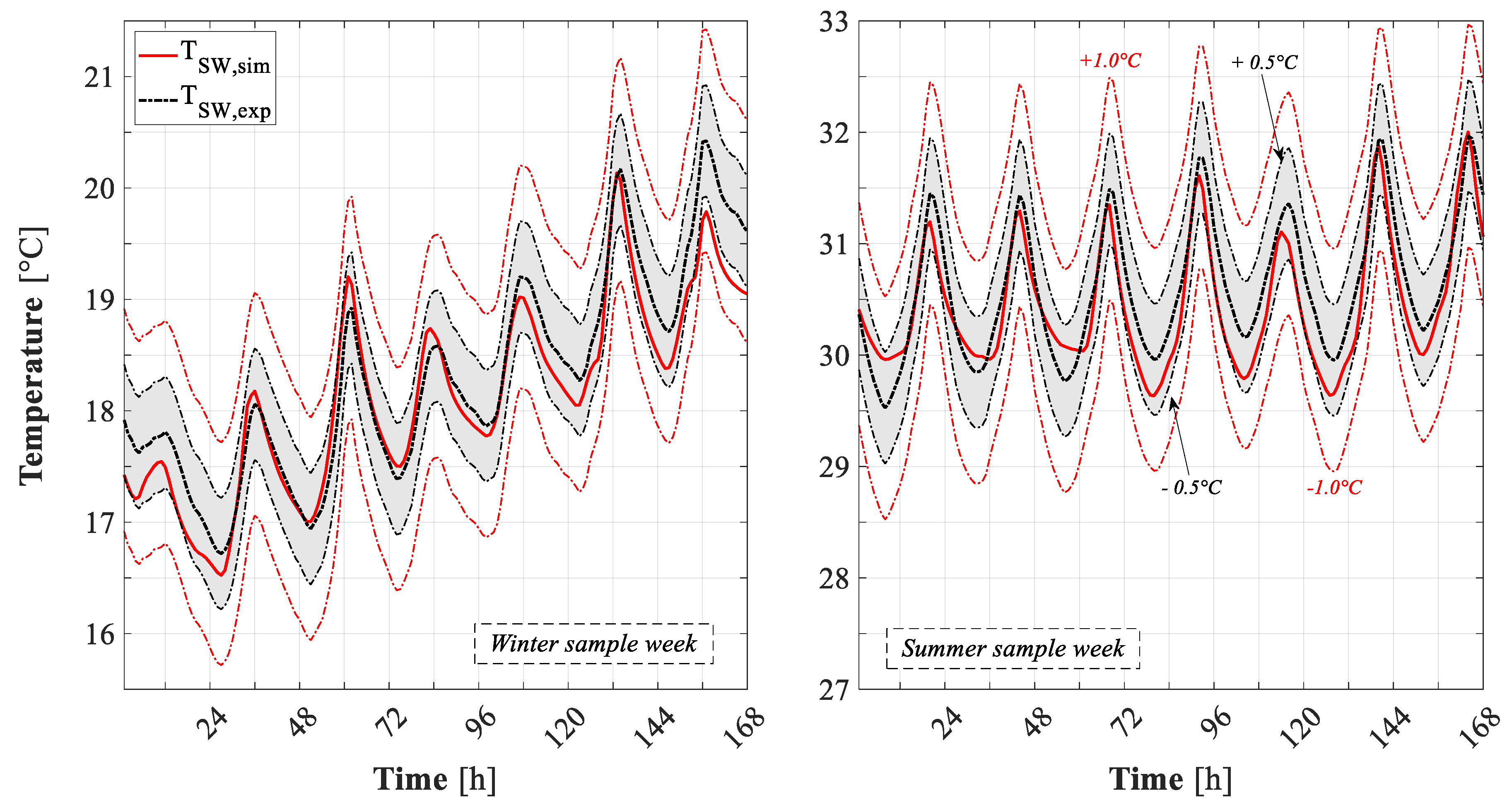
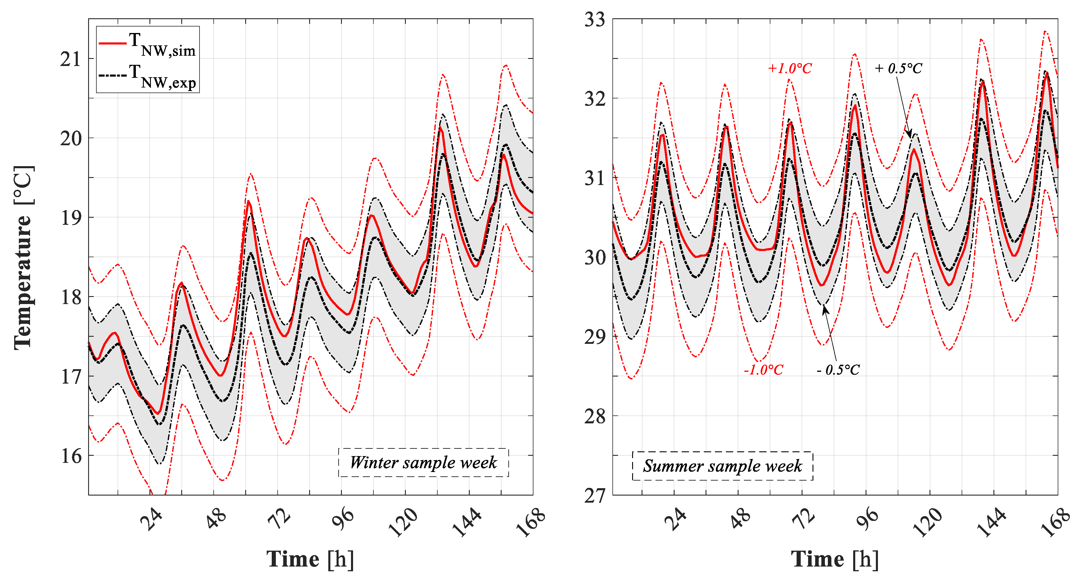
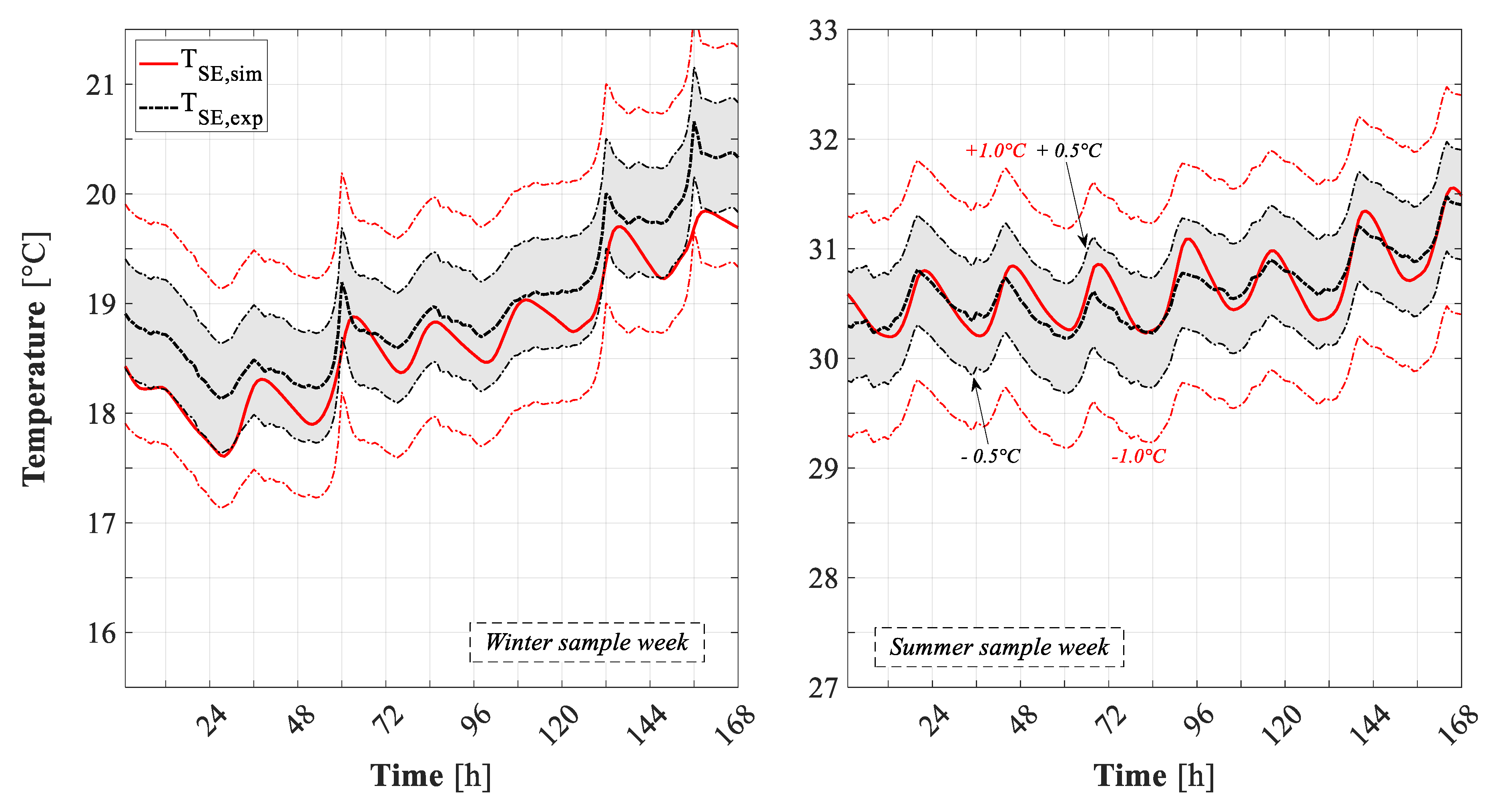
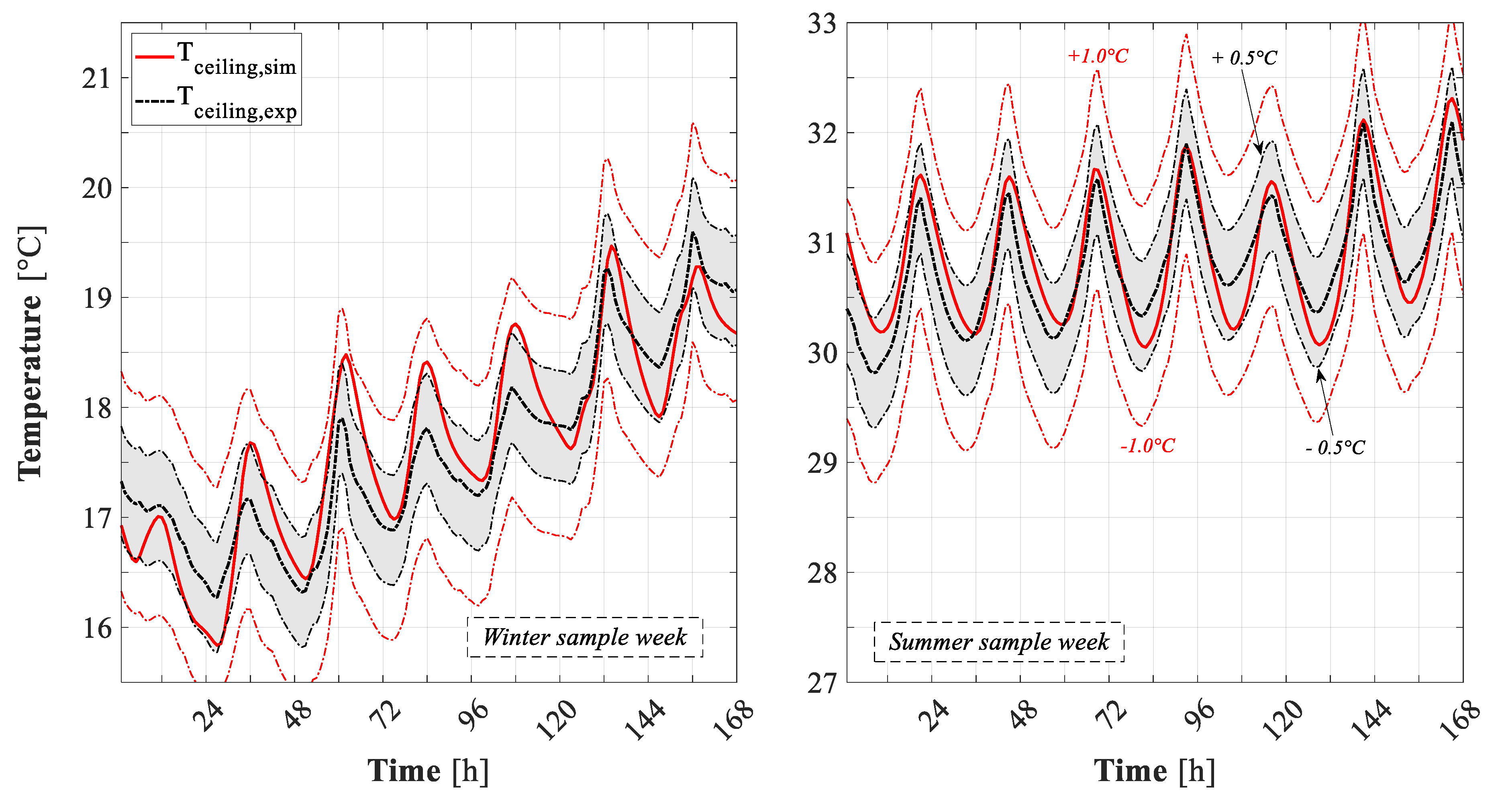
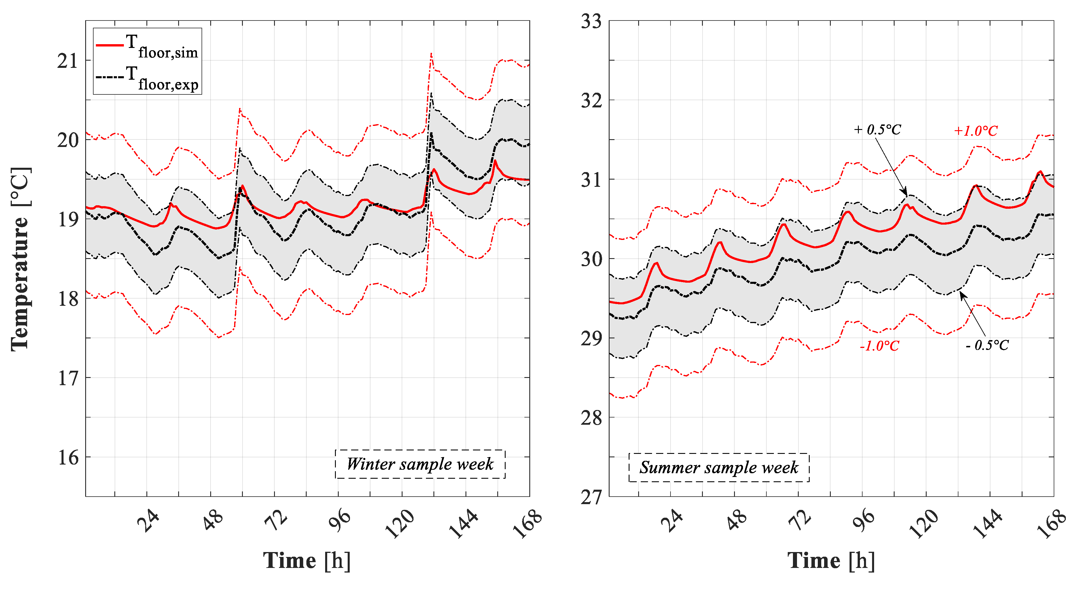
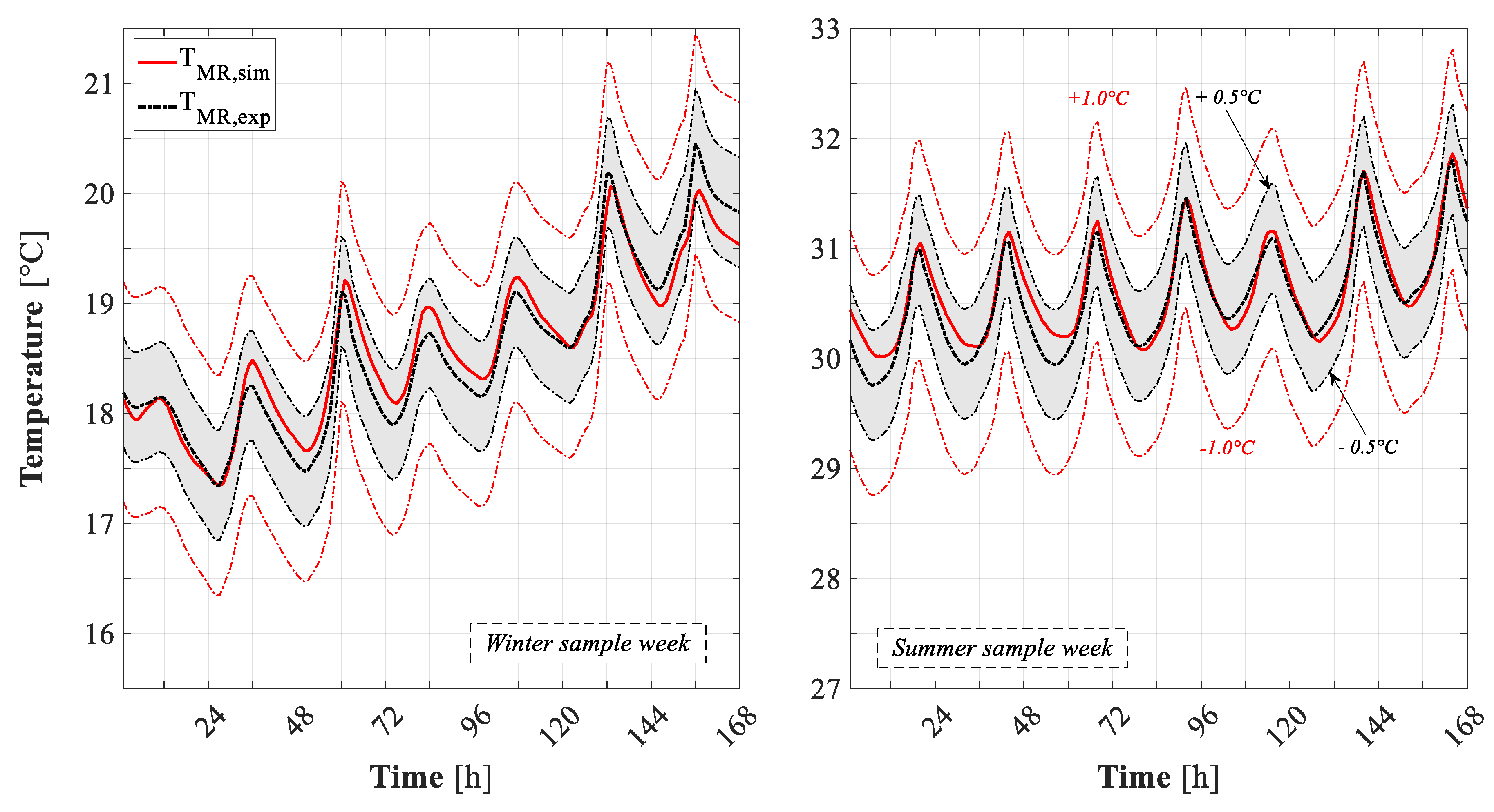
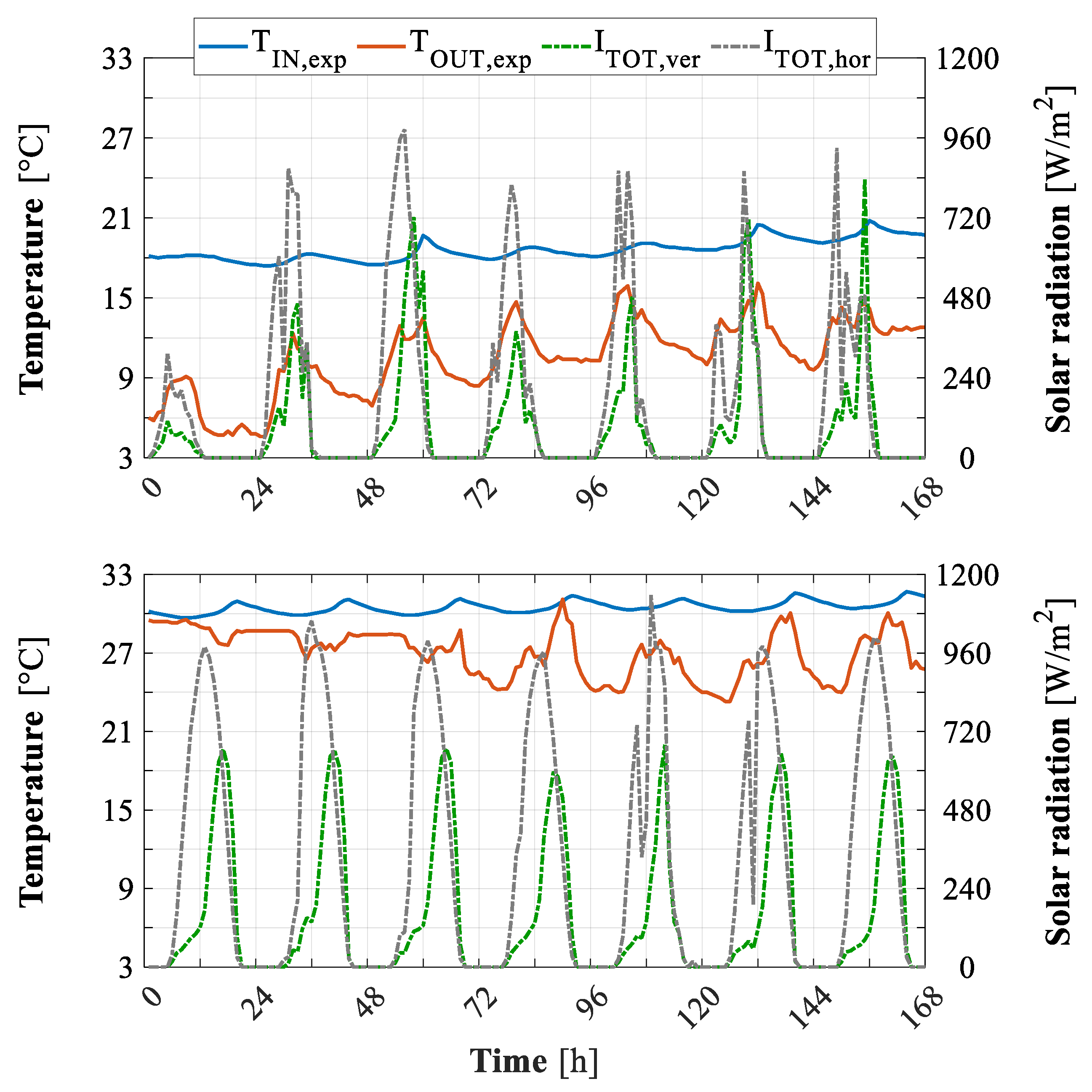
3.2. Experimental vs. Simulated Results
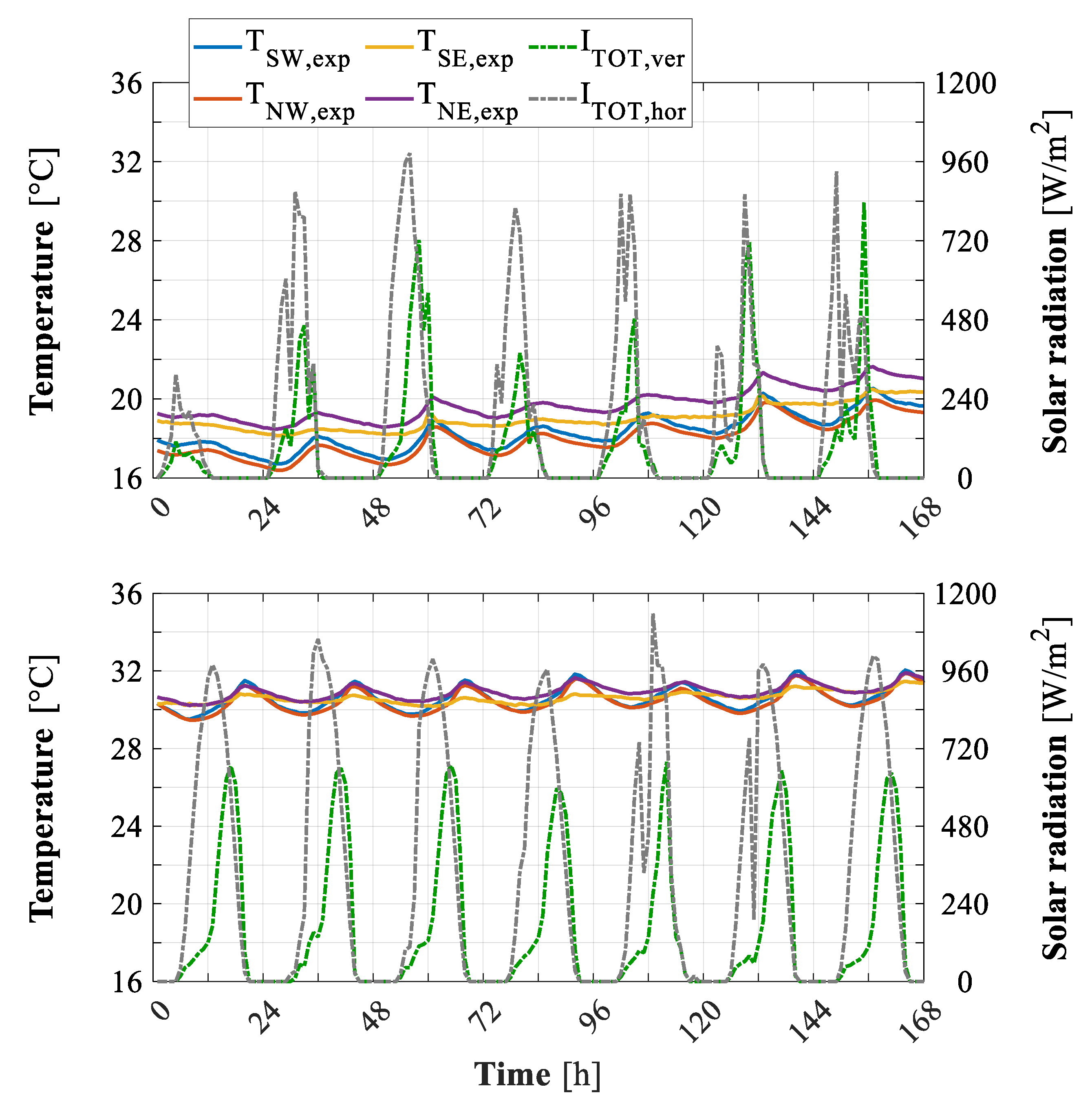
- global radiation on the outdoor horizontal roof surface, ITOThor, and vertical South-West façade, ITOTver. Note that, the global radiation on the vertical North-West façade is calculated starting from the measured global radiation on the outdoor horizontal surface;
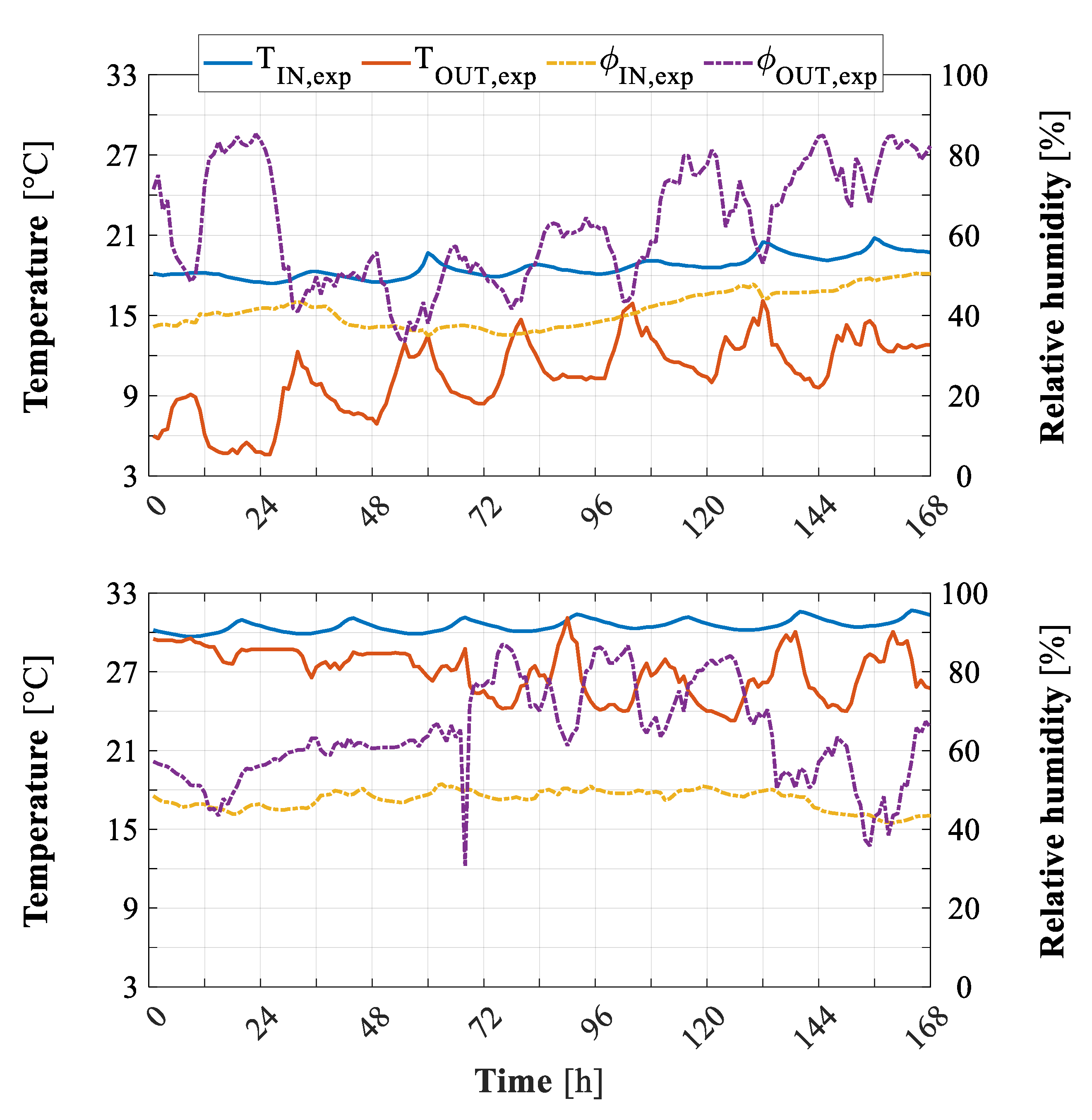
- outdoor air temperature, TOUT,exp;
- indoor air temperature of the corridor at the twelfth building floor limiting the SE wall (Figure 3). Such a temperature was implemented as boundary condition of the room SE wall;
- indoor air temperature of the building space at the eleventh floor. Such a temperature was implemented as boundary condition of the floor partition;
- internal surface temperature of the North-East wall, TNE,exp.
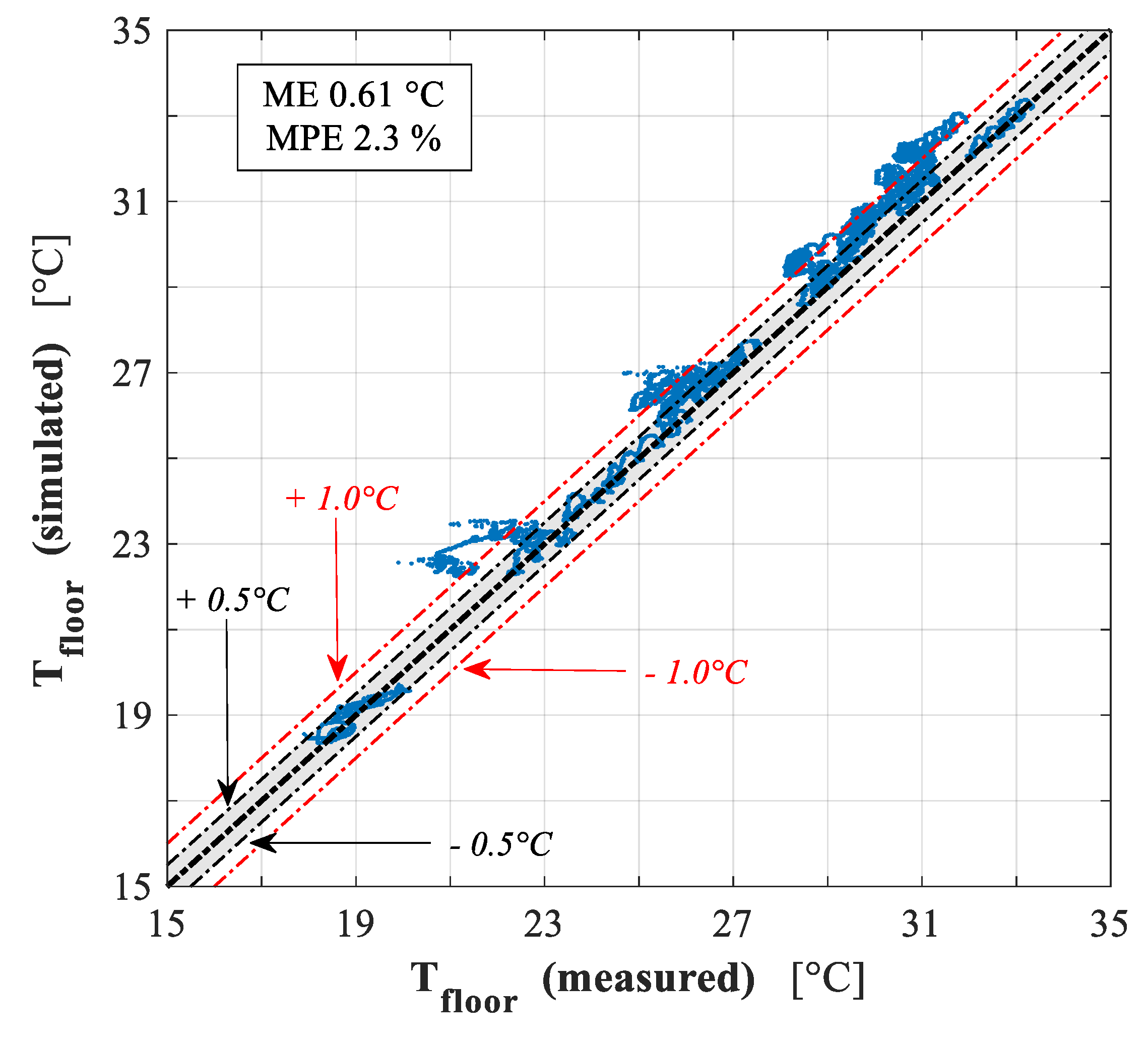
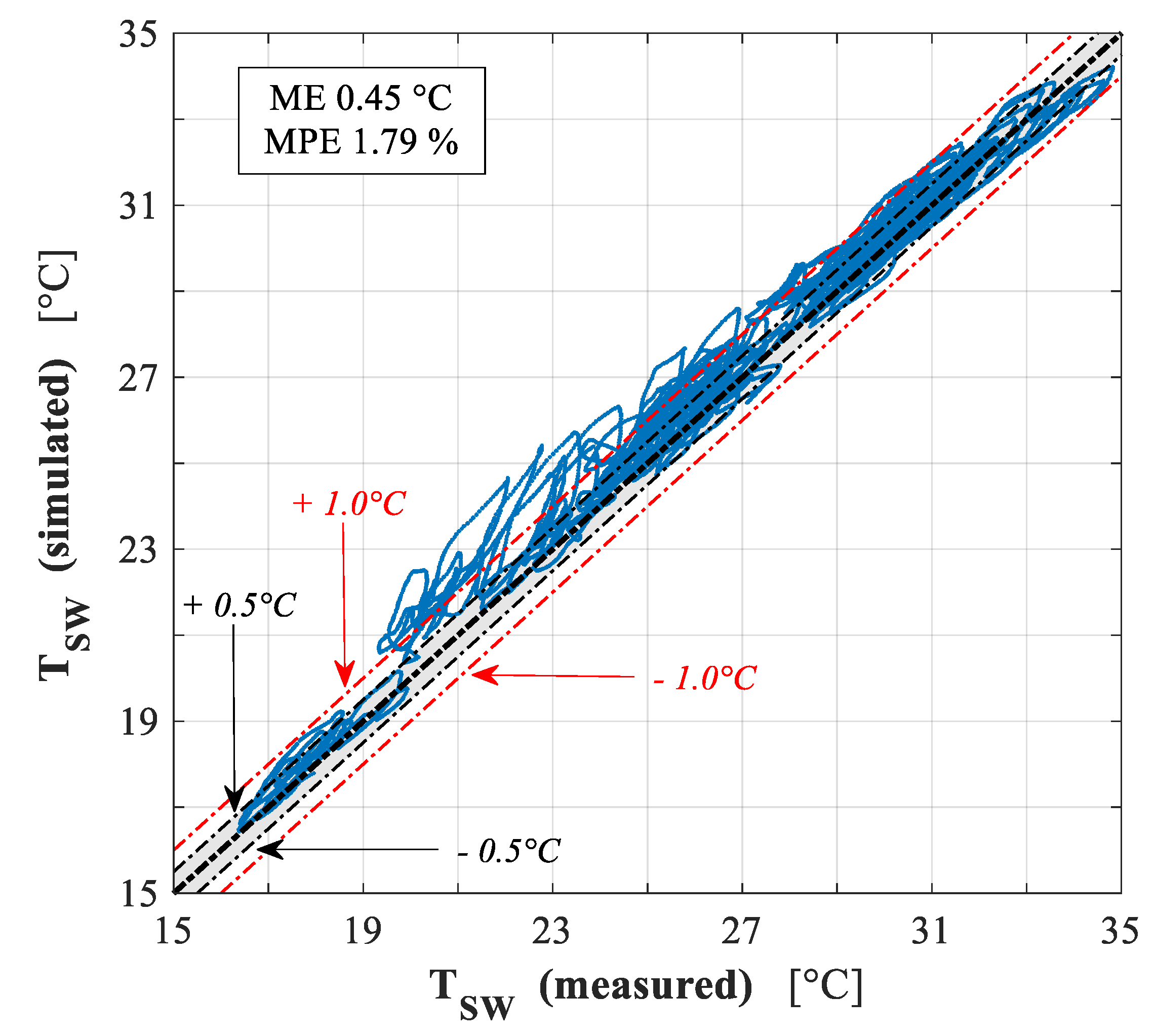
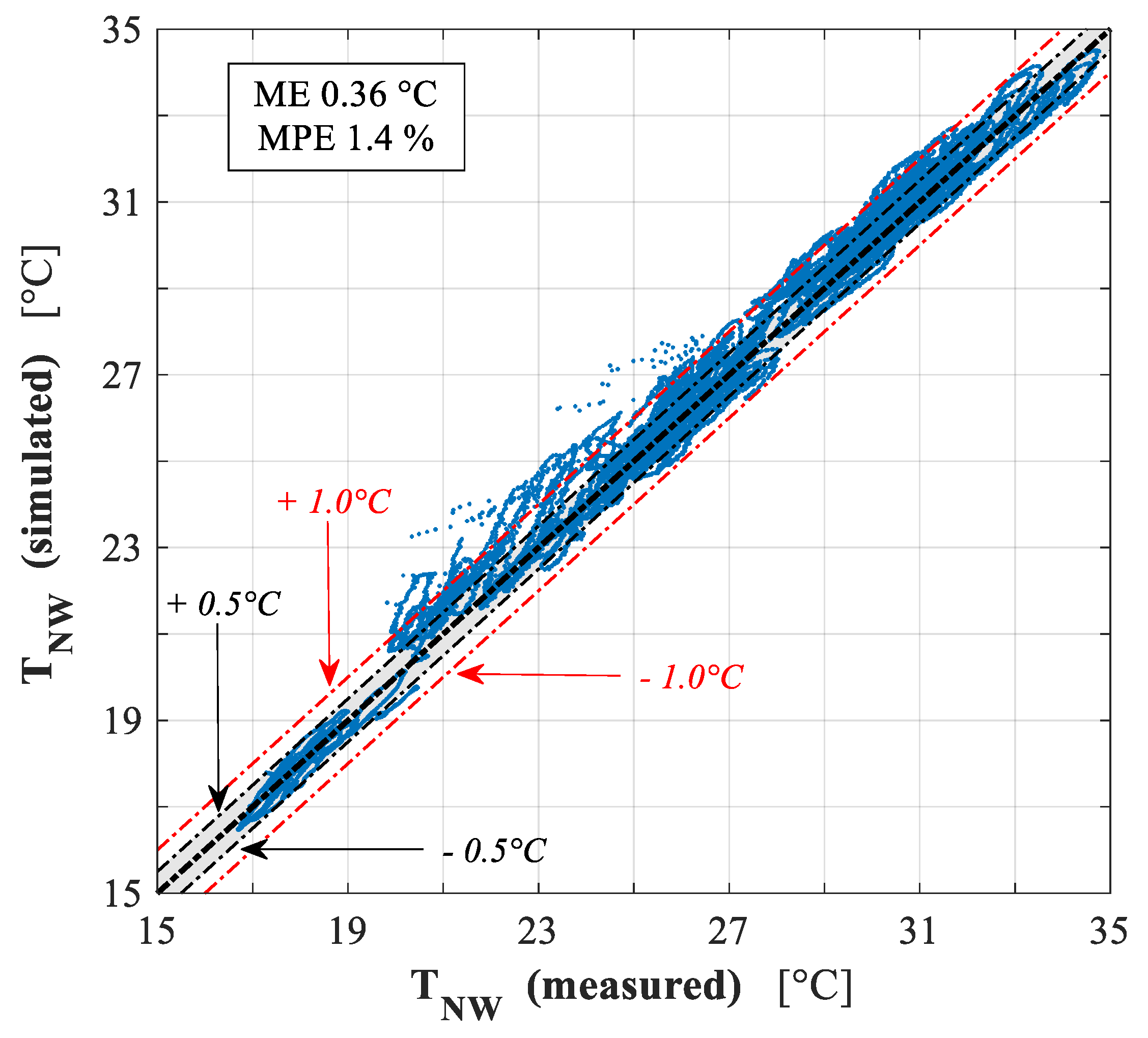
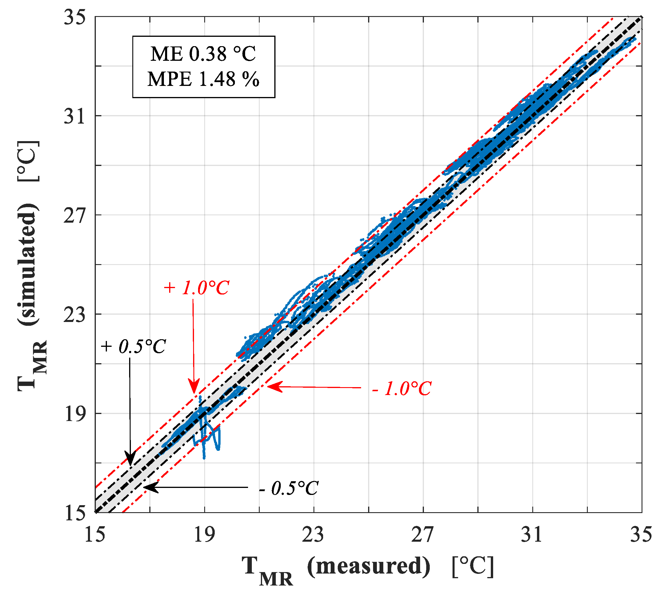
Error Analysis
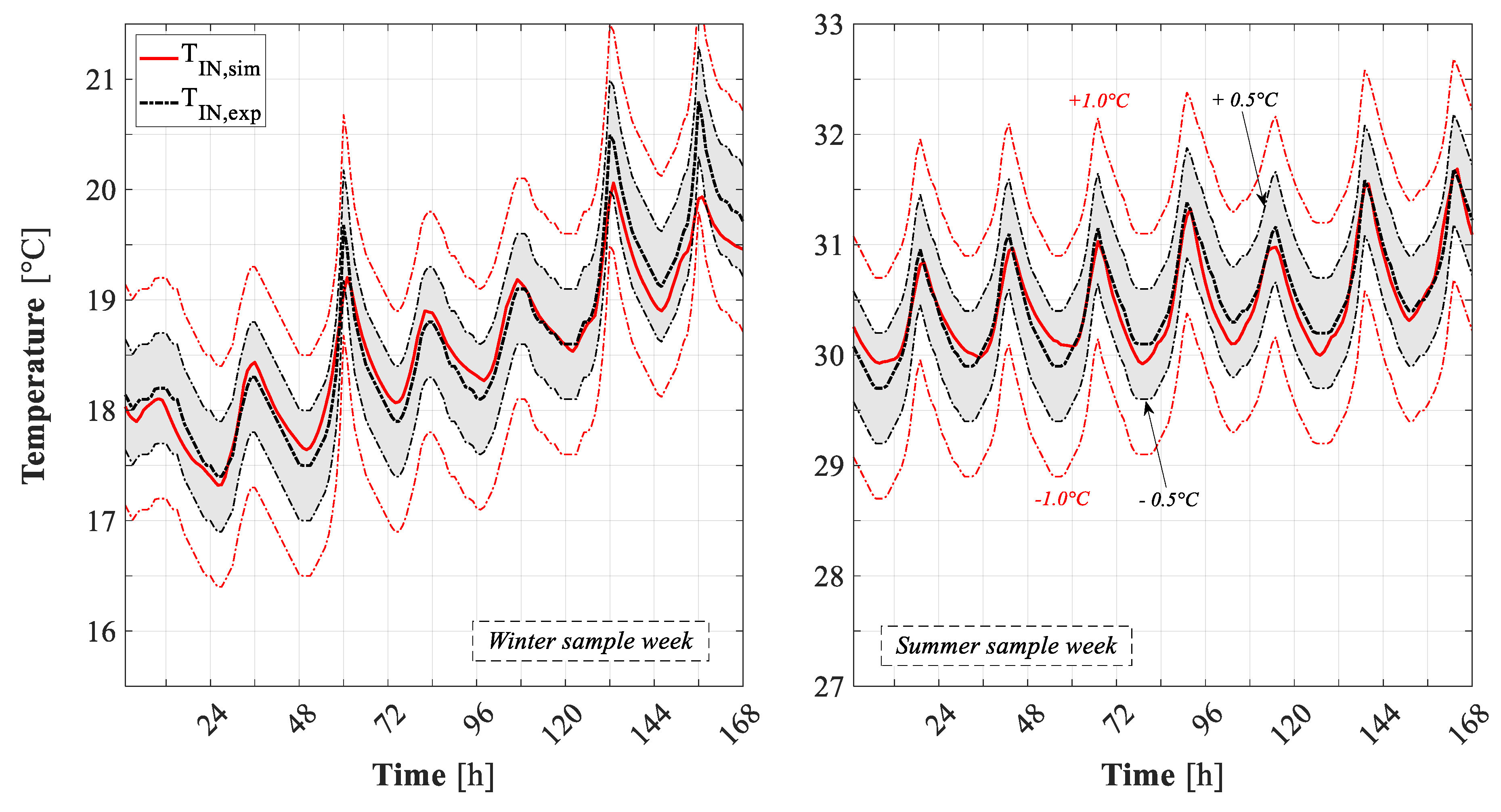
- Indoor air temperature (TIN): 0.39 °C and 1.47%;
- South-West wall temperature (TSW): 0.45 °C and 1.79%;
- North-West wall temperature (TNW): 0.36 °C and 1.40%;
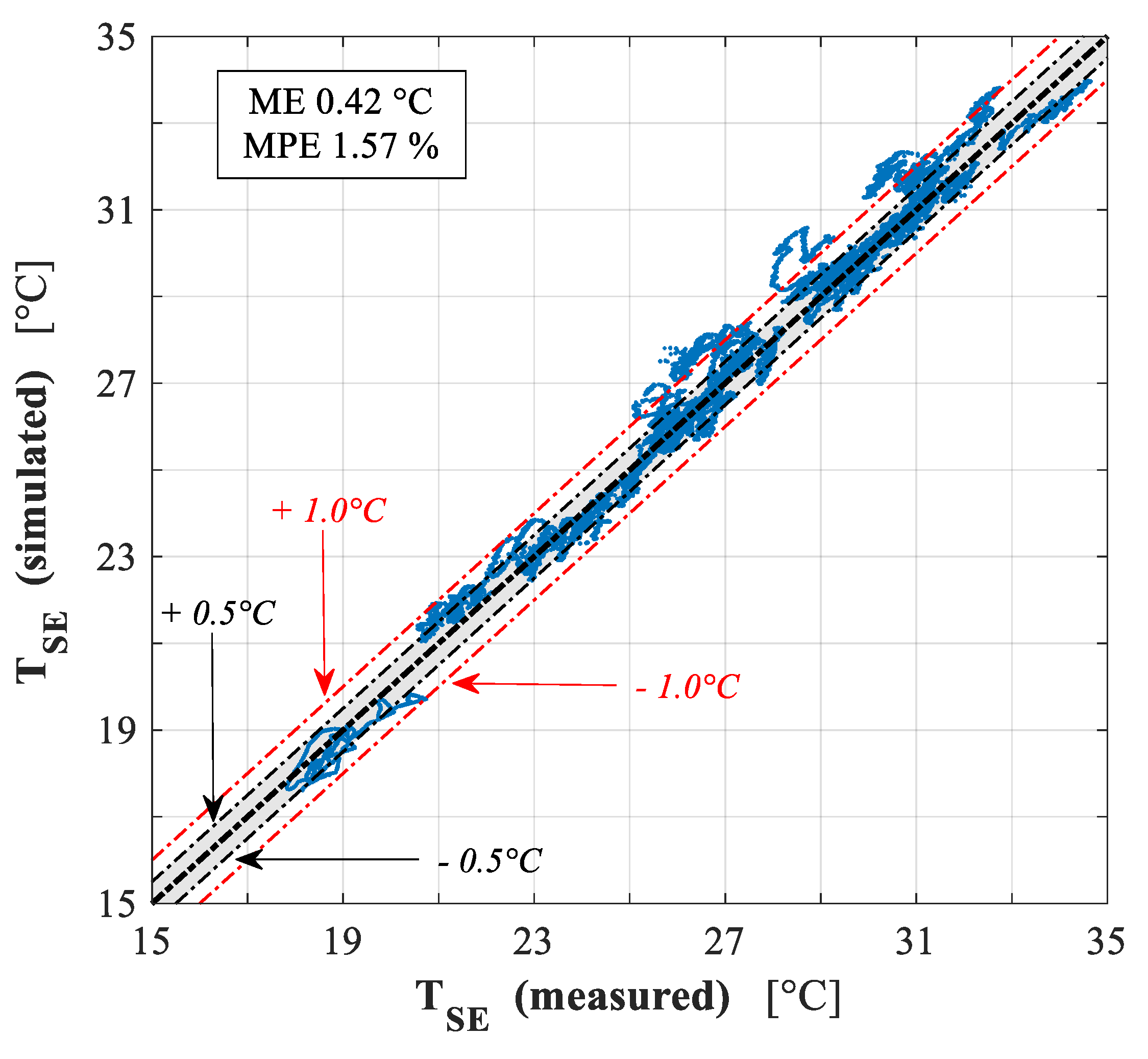
- South-East wall temperature (TSE): 0.42 °C and 1.57%;
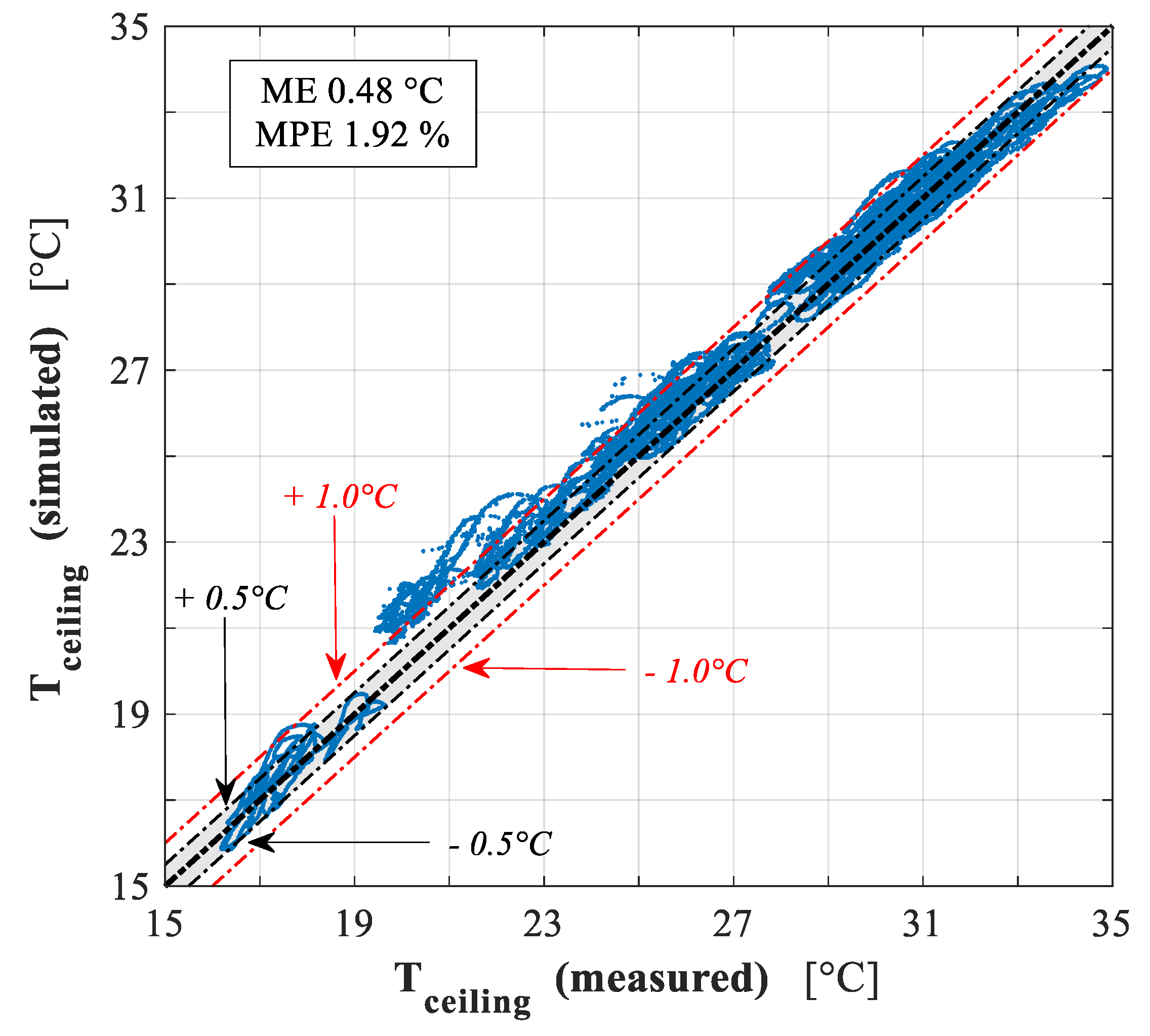
- Ceiling temperature (Tceiling): 0.48 °C and 1.92%;
- Floor temperature (Tfloor): 0.61 °C and 2.30%;
- Mean radiant temperature (TMR): 0.38 °C and 1.48%.
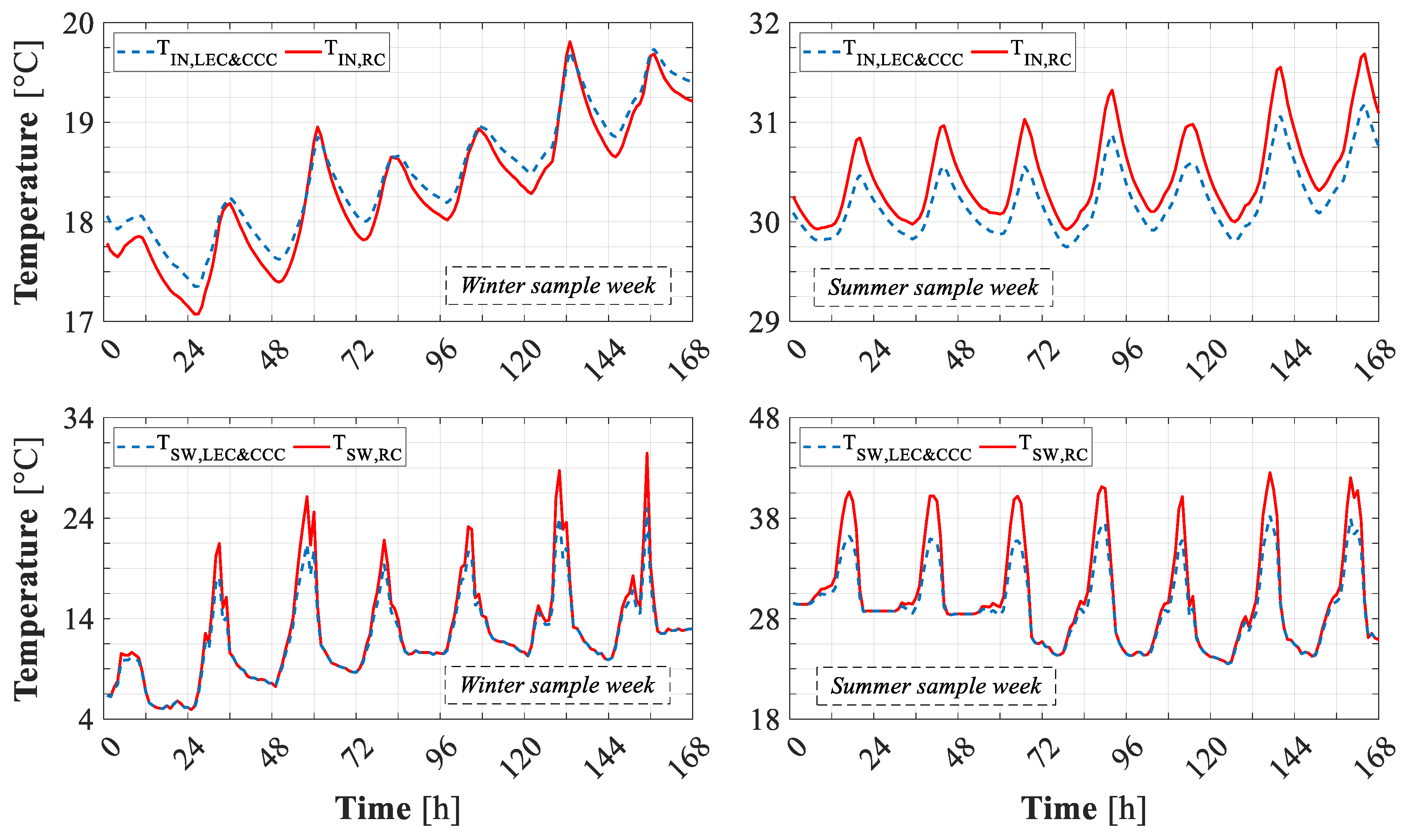
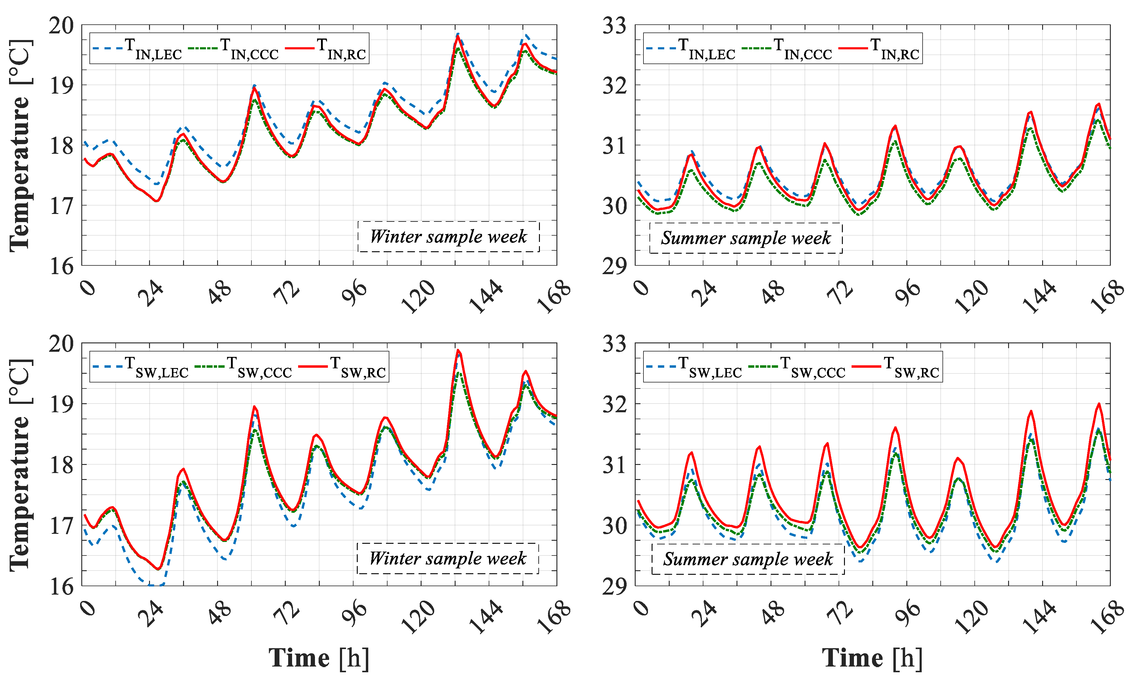
4. Case Study
- high solar reflective materials for reducing the outdoor surface temperature of buildings, and thus the related cooling peak and demand. Such materials (e.g., heat-reflective coatings, cool roof paints, etc.) are typically adopted for decreasing the summer overheating effect of building roofs due to the solar radiation;
- low-emittance materials to decrease the indoor surface temperature of buildings, and thus the related heating peak and demand. Such materials (low-e plasters, etc.) are typically adopted for reducing the winter heat dissipation effect due to the longwave infrared radiation energy absorbed by building perimeter walls.
- Reference Case (RC): αext is set to 0.3 for the exterior vertical surfaces and to 0.6 for the roof external surface, whereas LW of the interior surfaces is assumed to be 0.9.
- Low-Emissivity plaster Case (LEC): αext is set to 0.3 for the exterior vertical surfaces and to 0.6 for the roof (as for the reference case, RC), whereas LW of the interior surfaces is assumed to be 0.1 [87].
- Cool Coating Case (CCC): αext is calculated according to Equation (8), as a function of the solar reflectance data provided by reference [114] for the roof (as shown in Figure 27, varying from 0.33 to averagely 0.6), and by reference [116] for vertical surfaces coatings (varying from 0.15 to 0.3), whereas LW of the interior surfaces is assumed to be 0.9 (as for the reference case, RC);
Results and Discussion of the Case Study
5. Conclusions
Author Contributions
Funding
Conflicts of Interest
Nomenclature
| A | heat exchange surface area (m2) |
| C | thermal capacitance (J/K) |
| F | internal surfaces view factors matrix (-) |
| f | external surface view factor (-) |
| G | Gebhart’s matrix (-) |
| solar radiation flux (W/m2) | |
| identity matrix (-) | |
| I0 | vector of the total solar radiation directly received by the interior surfaces (W/m2) |
| Iint | vector of global solar radiation flux (W/m2) |
| M | building element nodes |
| N | building element layer nodes |
| Q | energy demand (Wh/y) |
| thermal load (W) | |
| R | thermal resistance (K/W) |
| T | temperature (K) |
| t | time (s) |
| Greeks letters | |
| absorption factor (-) | |
| emissivity (-) | |
| solar reflectivity matrix (-) | |
| reflectivity (-) | |
| Stefan-Boltzmann constant (W/m2/K4) | |
| Subscripts | |
| gain | building internal gain |
| in | the indoor air |
| m | the building element |
| n | the node of the thermal network |
| out | the outdoor air |
| sky | the sky vault |
| sp | the set point |
| tran | transmitted |
| vent | the dry air ventilation |
| cond | conduction |
| conv | convection |
| ext | external |
| int | internal |
| LW | long wave radiation |
| S | solar radiation |
References
- Council and European Parliament. Directive 2012/27/EU on Energy Efficiency, Amending Directives 2009/125/EC and 2010/30/EU and Repealing Directives 2004/8/EC and 2006/32/EC; Official Journal of the European Union: Brussels, Belgium, 2012. [Google Scholar]
- European Parliament. Directive 2010/31/EU of the European Parliament and of the Council on the Energy Performance of Buildings (Recast); Europan Parliament: Bruxelles, Belgium, 2010; Available online: https://eur-lex.europa.eu/eli/dir/2010/31/oj (accessed on 19 May 2010).
- Wang, N.; Phelan, P.E.; Harris, C.; Langevin, J.; Nelson, B.; Sawyer, K. Past visions, current trends, and future context: A review of building energy, carbon, and sustainability. Renew. Sustain. Energy Rev. 2018, 82, 976–993. [Google Scholar] [CrossRef]
- Wang, N.; Phelan, P.E.; Gonzalez, J.; Harris, C.; Henze, G.P.; Hutchinson, R.; Langevin, J.; Lazarus, M.A.; Nelson, B.; Pyke, C.; et al. Ten questions concerning future buildings beyond zero energy and carbon neutrality. Build. Environ. 2017, 119, 169–182. [Google Scholar] [CrossRef] [Green Version]
- Petrichenko, K.; Aden, N.; Tsakiris, A. Tools for Energy Efficiency in Buildings; A Guide for Policy-Makers and Experts; UNEP: Copenhagen, Denmark, 2016; Available online: https://orbit.dtu.dk/files/127199882/2016_11_Tools_Energy_Efficient_Buildings_PRINT.pdf (accessed on 1 November 2016).
- Becchio, C.; Corgnati, S.; Delmastro, C.; Fabi, V.; Lombardi, P. The role of nearly-zero energy buildings in the transition towards Post-Carbon Cities. Sustain. Cities Soc. 2016, 27, 324–337. [Google Scholar] [CrossRef]
- D’Agostino, D.; Cuniberti, B.; Bertoldi, P. Energy consumption and efficiency technology measures in European non-residential buildings. Energy Build. 2017, 153, 72–86. [Google Scholar] [CrossRef]
- Ferreira, M.; Almeida, M.; Rodrigues, A. Cost-optimal energy efficiency levels are the first step in achieving cost effective renovation in residential buildings with a nearly-zero energy target. Energy Build. 2016, 133, 724–737. [Google Scholar] [CrossRef]
- Negendahl, K. Building performance simulation in the early design stage: An introduction to integrated dynamic models. Autom. Constr. 2015, 54, 39–53. [Google Scholar] [CrossRef]
- Szalay, Z.; Zöld, A. Definition of nearly zero-energy building requirements based on a large building sample. Energy Policy 2014, 74, 510–521. [Google Scholar] [CrossRef]
- Nembrini, J.; Samberger, S.; Labelle, G. Parametric scripting for early design performance simulation. Energy Build. 2014, 68, 786–798. [Google Scholar] [CrossRef]
- Todorović, M.S. BPS, energy efficiency and renewable energy sources for buildings greening and zero energy cities planning: Harmony and ethics of sustainability. Energy Build. 2012, 48, 180–189. [Google Scholar] [CrossRef]
- Soares, N.; Bastos, J.; Pereira, L.D.; Soares, A.; Amaral, A.; Asadi, E.; Rodrigues, E.; Lamas, F.; Monteiro, H.; Lopes, M.; et al. A review on current advances in the energy and environmental performance of buildings towards a more sustainable built environment. Renew. Sustain. Energy Rev. 2017, 77, 845–860. [Google Scholar] [CrossRef]
- Yang, G.; Wenjie, J.; Borong, L.; Jiakie, H.; Yingxin, Z. Building energy performance diagnosis using energy bills and weather data. Energy Build. 2018, 172, 181–191. [Google Scholar]
- Diakaki, C.; Grigoroudis, E.; Kolokotsa, D. Towards a multi-objective optimization approach for improving energy efficiency in buildings. Energy Build. 2008, 40, 1747–1754. [Google Scholar] [CrossRef]
- Crawley, D.B.; Hand, J.W.; Kummert, M.; Griffith, B.T. Contrasting the capabilities of building energy performance simulation programs. Build. Environ. 2008, 43, 661–673. [Google Scholar] [CrossRef] [Green Version]
- IBPSA-USA. Building Energy Software Tools. 2018. Available online: www.buildingenergysoftwaretools.com/ (accessed on 28 October 2018).
- Attia, S.; Hensen, J.L.; Beltrán, L.; De Herde, A. Selection criteria for building performance simulation tools: Contrasting architects’ and engineers’ needs. J. Build. Perform. Simul. 2012, 5, 155–169. [Google Scholar] [CrossRef]
- Connolly, D.; Lund, H.; Mathiesen, B.V.; Leahy, M. A review of computer tools for analysing the integration of renewable energy into various energy systems. Appl. Energy 2010, 87, 1059–1082. [Google Scholar] [CrossRef]
- Mahmud, K.; Amin, U.; Hossain, M.; Ravishankar, J. Computational tools for design, analysis, and management of residential energy systems. Appl. Energy 2018, 221, 535–556. [Google Scholar] [CrossRef]
- Allegrini, J.; Orehounig, K.; Mavromatidis, G.; Ruesch, F.; Dorer, V.; Evins, R. A review of modelling approaches and tools for the simulation of district-scale energy systems. Renew. Sustain. Energy Rev. 2015, 52, 1391–1404. [Google Scholar] [CrossRef]
- Lucia, C.V.; Laura, P.A. Uses of dynamic simulation to predict thermal-energy performance of buildings and districts: A review. Wiley Interdiscip. Rev. Energy Environ. 2018, 7, e269. [Google Scholar]
- Attia, S.; Hamdy, M.; O’Brien, W.; Carlucci, S. Assessing gaps and needs for integrating building performance optimization tools in net zero energy buildings design. Energy Build. 2013, 60, 110–124. [Google Scholar] [CrossRef] [Green Version]
- Wang, H.; Zhai, Z. Advances in building simulation and computational techniques: A review between 1987 and 2014. Energy Build. 2016, 128, 319–335. [Google Scholar] [CrossRef]
- Fumo, N. A review on the basics of building energy estimation. Renew. Sustain. Energy Rev. 2014, 31, 53–60. [Google Scholar] [CrossRef]
- Bigot, D.; Miranville, F.; Fakra, A.; Boyer, H. A nodal thermal model for photovoltaic systems: Impact on building temperature fields and elements of validation for tropical and humid climatic conditions. Energy Build. 2009, 41, 1117–1126. [Google Scholar] [CrossRef]
- Bigot, D.; Miranville, F.; Boyer, H.; Bojic, M.; Guichard, S.; Jean, A. Model optimization and validation with experimental data using the case study of a building equipped with photovoltaic panel on roof: Coupling of the building thermal simulation code ISOLAB with the generic optimization program GenOpt. Energy Build. 2013, 58, 333–347. [Google Scholar] [CrossRef]
- Guichard, S.; Miranville, F.; Bigot, D.; Boyer, H. A thermal model for phase change materials in a building roof for a tropical and humid climate: Model description and elements of validation. Energy Build. 2014, 70, 71–80. [Google Scholar] [CrossRef] [Green Version]
- Lee, E.S.; Geisler-Moroder, D.; Ward, G. Modeling the direct sun component in buildings using matrix algebraic approaches: Methods and validation. Sol. Energy 2018, 160, 380–395. [Google Scholar] [CrossRef] [Green Version]
- Shen, P.; Braham, W.; Yi, Y. Development of a lightweight building simulation tool using simplified zone thermal coupling for fast parametric study. Appl. Energy 2018, 223, 188–214. [Google Scholar] [CrossRef]
- Clarke, J.; Hensen, J.; Hensen, J. Integrated building performance simulation: Progress, prospects and requirements. Build. Environ. 2015, 91, 294–306. [Google Scholar] [CrossRef] [Green Version]
- Attia, S.; Gratia, E.; De Herde, A.; Hensen, J.L. Simulation-based decision support tool for early stages of zero-energy building design. Energy Build. 2012, 49, 2–15. [Google Scholar] [CrossRef] [Green Version]
- Fonseca i Casas, P.; Casas, A.F.; Garrido, N.; Casanovas, J. Formal simulation model to optimize building sustainability. Adv. Eng. Softw. 2014, 69, 62–74. [Google Scholar] [CrossRef] [Green Version]
- Ioannidis, Z.; Buonomano, A.; Athienitis, A.; Stathopoulos, T. Modeling of double skin façades integrating photovoltaic panels and automated roller shades: Analysis of the thermal and electrical performance. Energy Build. 2017, 154, 618–632. [Google Scholar] [CrossRef]
- Capizzi, G.; Sciuto, G.L.; Cammarata, G.; Cammarata, M. Thermal transients simulations of a building by a dynamic model based on thermal-electrical analogy: Evaluation and implementation issue. Appl. Energy 2017, 199, 323–334. [Google Scholar] [CrossRef]
- Figueiredo, A.; Kämpf, J.; Vicente, R.; Oliveira, R.; Silva, T. Comparison between monitored and simulated data using evolutionary algorithms: Reducing the performance gap in dynamic building simulation. J. Build. Eng. 2018, 17, 96–106. [Google Scholar] [CrossRef]
- Ryan, E.M.; Sanquist, T.F. Validation of building energy modeling tools under idealized and realistic conditions. Energy Build. 2012, 47, 375–382. [Google Scholar] [CrossRef]
- Van der Veken, J.; Saelens, D.; Verbeeck, G.; Hens, H. Comparison of Steady -State and Dynamic Building Energy Simulation Programs. In Proceedings of the International Buildings IX ASHRAE Conference on the Performance of Exterior Envelopes of Whole Buildings, Nashville, Tennessee, December 2004; Available online: https://lirias.kuleuven.be/retrieve/39797 (accessed on 27 October 2019).
- Melo, A.; Costola, D.; Lamberts, R.; Hensen, J.; Hensen, J. Assessing the accuracy of a simplified building energy simulation model using BESTEST: The case study of Brazilian regulation. Energy Build. 2012, 45, 219–228. [Google Scholar] [CrossRef] [Green Version]
- Mantesi, E.; Hopfe, C.J.; Cook, M.J.; Glass, J.; Strachan, P. The modelling gap: Quantifying the discrepancy in the representation of thermal mass in building simulation. Build. Environ. 2018, 131, 74–98. [Google Scholar] [CrossRef] [Green Version]
- IEA SHC. Testing and Validation of Building Energy Simulation Tools. Comparative Test Case Specification. In Annex 43/SHC Task 34 2003–2007; Department of Civil Engineering, Aalborg University: Aalborg, Denmark, 2004; Available online: https://vbn.aau.dk/en/projects/iea-shc-task-34ecbcs-annex-43-testing-and-validation-of-building- (accessed on 13 August 2001).
- Coakley, D.; Raftery, P.; Keane, M. A review of methods to match building energy simulation models to measured data. Renew. Sustain. Energy Rev. 2014, 37, 123–141. [Google Scholar] [CrossRef] [Green Version]
- Judkoffm, R.; Wortman, D.; O’Doherty, B.; Burch, J. A Methodology for Validating Building Energy Analysis Simulations, SERI/TR-254-1508; Solar Energy Research Institute (now National Renewable Energy Laboratory): Golden, CO, USA, 1983. [Google Scholar]
- Neymark, J.; Judkoff, R.; Knabe, G.; Le, H.-T.; Dürig, M.; Glass, A.; Zweifel, G. Applying the building energy simulation test (BESTEST) diagnostic method to verification of space conditioning equipment models used in whole-building energy simulation programs. Energy Build. 2002, 34, 917–931. [Google Scholar] [CrossRef]
- Ren, Z.; Chen, D.; James, M. Evaluation of a whole-house energy simulation tool against measured data. Energy Build. 2018, 171, 116–130. [Google Scholar] [CrossRef]
- Ben-Nakhi, A.E.; Aasem, E.O. Development and integration of a user friendly validation module within whole building dynamic simulation. Energy Convers. Manag. 2003, 44, 53–64. [Google Scholar] [CrossRef]
- Lomas, K.; Eppel, H.; Martin, C.; Bloomfield, D. Empirical validation of building energy simulation programs. Energy Build. 1997, 26, 253–275. [Google Scholar] [CrossRef]
- Nageler, P.; Schweiger, G.; Pichler, M.; Brandl, D.; Mach, T.; Heimrath, R.; Schranzhofer, H.; Hochenauer, C. Validation of dynamic building energy simulation tools based on a real test-box with thermally activated building systems (TABS). Energy Build. 2018, 168, 42–55. [Google Scholar] [CrossRef]
- Zhu, Q.; Li, A.; Xie, J.; Li, W.; Xu, X. Experimental validation of a semi-dynamic simplified model of active pipe-embedded building envelope. Int. J. Therm. Sci. 2016, 108, 70–80. [Google Scholar] [CrossRef] [Green Version]
- Romaní, J.; Cabeza, L.F.; De Gracia, A. Development and experimental validation of a transient 2D numeric model for radiant walls. Renew. Energy 2018, 115, 859–870. [Google Scholar] [CrossRef] [Green Version]
- Loutzenhiser, P.G.; Manz, H.; Moosberger, S.; Maxwell, G.M. An empirical validation of window solar gain models and the associated interactions. Int. J. Therm. Sci. 2009, 48, 85–95. [Google Scholar] [CrossRef]
- Malet-Damour, B.; Guichard, S.; Bigot, D.; Boyer, H. Study of tubular daylight guide systems in buildings: Experimentation, modelling and validation. Energy Build. 2016, 129, 308–321. [Google Scholar] [CrossRef]
- Alaidroos, A.; Krarti, M. Experimental validation of a numerical model for ventilated wall cavity with spray evaporative cooling systems for hot and dry climates. Energy Build. 2016, 131, 207–222. [Google Scholar] [CrossRef]
- Zingre, K.T.; Yang, E.-H.; Wan, M.P. Dynamic thermal performance of inclined double-skin roof: Modeling and experimental investigation. Energy 2017, 133, 900–912. [Google Scholar] [CrossRef]
- Blanco, J.M.; Arriaga, P.; Rojí, E.; Cuadrado, J.; Chandro, E.R. Investigating the thermal behavior of double-skin perforated sheet façades: Part A: Model characterization and validation procedure. Build. Environ. 2014, 82, 50–62. [Google Scholar] [CrossRef]
- Anđelković, A.S.; Mujan, I.; Dakić, S. Experimental validation of a EnergyPlus model: Application of a multi-storey naturally ventilated double skin façade. Energy Build. 2016, 118, 27–36. [Google Scholar] [CrossRef]
- Sandels, C.; Brodén, D.; Widén, J.; Nordström, L.; Andersson, E. Modeling office building consumer load with a combined physical and behavioral approach: Simulation and validation. Appl. Energy 2016, 162, 472–485. [Google Scholar] [CrossRef]
- Attia, S. State of the Art of Existing Early Design Simulation Tools for Net Zero Energy Buildings: A Comparison of Ten Tools; Université Catholique de Louvain: Louvain La Neuve, Belgium, 2011. [Google Scholar]
- Lirola, J.M.; Castañeda, E.; Lauret, B.; Khayet, M. A review on experimental research using scale models for buildings: Application and methodologies. Energy Build. 2017, 142, 72–110. [Google Scholar] [CrossRef] [Green Version]
- Cattarin, G.; Pagliano, L.; Causone, F.; Kindinis, A. Empirical and comparative validation of an original model to simulate the thermal behaviour of outdoor test cells. Energy Build. 2018, 158, 1711–1723. [Google Scholar] [CrossRef]
- Strachan, P.; Svehla, K.; Heusler, I.; Kersken, M. Whole model empirical validation on a full-scale building. J. Build. Perform. Simul. 2016, 9, 331–350. [Google Scholar] [CrossRef]
- CEN European Committee for Standardizations. EN 15265:2007—Thermal Performance of Buildings—Calculation of Energy Use for Space Heating and Cooling; General Criteria and Validation Procedures: Brussels, Belgium, 2007. [Google Scholar]
- ASHRAE American Society of Heating Refrigerating and Air-Conditioning Engineers. ANSI/ASHRAE Standard 90.1-2010: Energy Standard for Building Except Low-rise Residential Buildings; Atlanta, GA, USA, 2010; Available online: https://www.usailighting.com/stuff/contentmgr/files/1/b90ce247855d0f17438484c003877338/misc/ashrae_90_1_2010.pdf (accessed on 27 October 2010).
- Al-Homoud, M.S. Computer-aided building energy analysis techniques. Build. Environ. 2001, 36, 421–433. [Google Scholar] [CrossRef]
- Judkoff, R.; Neymark, J. International Energy Agency Building Energy Simulation Test (BESTEST) and Diagnostic Method; NREL/TP-472-62312005; ASHRAE: Golden, CO, USA, 1995. Available online: https://www.osti.gov/biblio/90674-international-energy-agency-building-energy-simulation-test-bestest-diagnostic-method (accessed on 1 February 1995).
- ANSI/ASHRAE Standard 140-2014: Standard Method of Test for the Evaluation of Building Energy Analysis Computer Programs; Atlanta, GA, USA, 2014; Available online: https://webstore.ansi.org/standards/ashrae/ansiashraestandard1402017 (accessed on 1 February 2007).
- Corgnati, S.P.; Fabrizio, E.; Raimondo, D.; Filippi, M. Categories of indoor environmental quality and building energy demand for heating and cooling. Build. Simul. 2011, 4, 97–105. [Google Scholar] [CrossRef]
- Jradi, M.; Arendt, K.; Sangogboye, F.; Mattera, C.; Markoska, E.; Kjærgaard, M.; Veje, C.; Jørgensen, B. ObepME: An online building energy performance monitoring and evaluation tool to reduce energy performance gaps. Energy Build. 2018, 166, 196–209. [Google Scholar] [CrossRef] [Green Version]
- Jaffal, I.; Inard, C. A metamodel for building energy performance. Energy Build. 2017, 151, 501–510. [Google Scholar] [CrossRef]
- Andersen, R.K.; Fabi, V.; Corgnati, S.P. Predicted and actual indoor environmental quality: Verification of occupants’ behaviour models in residential buildings. Energy Build. 2016, 127, 105–115. [Google Scholar] [CrossRef]
- Čekon, M.; Čurpek, J. A transparent insulation façade enhanced with a selective absorber: A cooling energy load and validated building energy performance prediction model. Energy Build. 2019, 183, 266–282. [Google Scholar] [CrossRef]
- Buonomano, A.; Palombo, A. Building energy performance analysis by an in-house developed dynamic simulation code: An investigation for different case studies. Appl. Energy 2014, 113, 788–807. [Google Scholar] [CrossRef]
- Buonomano, A.; Montanaro, U.; Palombo, A.; Santini, S. Dynamic building energy performance analysis: A new adaptive control strategy for stringent thermohygrometric indoor air requirements. Appl. Energy 2016, 163, 361–386. [Google Scholar] [CrossRef]
- Buonomano, A.; Montanaro, U.; Palombo, A.; Santini, S. Adaptive Control for Building Thermo-hygrometric Analysis: A Novel Dynamic Simulation Code for Indoor Spaces with Multi-enclosed Thermal Zones. Energy Procedia 2015, 78, 2190–2195. [Google Scholar] [CrossRef] [Green Version]
- Buonomano, A.; Calise, F.; Palombo, A. Solar heating and cooling systems by CPVT and ET solar collectors: A novel transient simulation model. Appl. Energy 2013, 103, 588–606. [Google Scholar] [CrossRef]
- Athienitis, A.K.; Barone, G.; Buonomano, A.; Palombo, A. Assessing active and passive effects of façade building integrated photovoltaics/thermal systems: Dynamic modelling and simulation. Appl. Energy 2018, 209, 355–382. [Google Scholar] [CrossRef]
- Buonomano, A.; Montanaro, U.; Palombo, A.; Santini, S. Temperature and humidity adaptive control in multi-enclosed thermal zones under unexpected external disturbances. Energy Build. 2017, 135, 263–285. [Google Scholar] [CrossRef]
- Buonomano, A.; Calise, F.; Palombo, A. Solar heating and cooling systems by absorption and adsorption chillers driven by stationary and concentrating photovoltaic/thermal solar collectors: Modelling and simulation. Renew. Sustain. Energy Rev. 2018, 81, 1112–1146. [Google Scholar] [CrossRef]
- Barone, G.; Buonomano, A.; Forzano, C.; Palombo, A. WLHP Systems in Commercial Buildings: A Case Study Analysis Based on a Dynamic Simulation Approach. Am. J. Eng. Appl. Sci. 2016, 9, 659–668. [Google Scholar] [CrossRef] [Green Version]
- Marino, C.; Minichiello, F.; Bahnfleth, W. The influence of surface finishes on the energy demand of HVAC systems for existing buildings. Energy Build. 2015, 95, 70–79. [Google Scholar] [CrossRef]
- Park, B.; Krarti, M. Energy performance analysis of variable reflectivity envelope systems for commercial buildings. Energy Build. 2016, 124, 88–98. [Google Scholar] [CrossRef]
- Santamouris, M. Cooling the cities—A review of reflective and green roof mitigation technologies to fight heat island and improve comfort in urban environments. Sol. Energy 2014, 103, 682–703. [Google Scholar] [CrossRef]
- Shi, Z.; Zhang, X. Analyzing the effect of the longwave emissivity and solar reflectance of building envelopes on energy-saving in buildings in various climates. Sol. Energy 2011, 85, 28–37. [Google Scholar] [CrossRef]
- Joudi, A.; Svedung, H.; Cehlin, M.; Rönnelid, M. Reflective coatings for interior and exterior of buildings and improving thermal performance. Appl. Energy 2013, 103, 562–570. [Google Scholar] [CrossRef]
- Jelle, B.P.; Kalnæs, S.E.; Gao, T. Low-emissivity materials for building applications: A state-of-the-art review and future research perspectives. Energy Build. 2015, 96, 329–356. [Google Scholar] [CrossRef] [Green Version]
- Pisello, A.L. State of the art on the development of cool coatings for buildings and cities. Sol. Energy 2017, 144, 660–680. [Google Scholar] [CrossRef]
- Ibrahim, M.; Bianco, L.; Ibrahim, O.; Wurtz, E. Low-emissivity coating coupled with aerogel-based plaster for walls’ internal surface application in buildings: Energy saving potential based on thermal comfort assessment. J. Build. Eng. 2018, 18, 454–466. [Google Scholar] [CrossRef]
- Zinzi, M. Exploring the potentialities of cool facades to improve the thermal response of Mediterranean residential buildings. Sol. Energy 2016, 135, 386–397. [Google Scholar] [CrossRef]
- Alonso, C.; Martín-Consuegra, F.; Oteiza, I.; Asensio, E.; Pérez, G.; Martínez, I.; Frutos, B. Effect of façade surface finish on building energy rehabilitation. Sol. Energy 2017, 146, 470–483. [Google Scholar] [CrossRef]
- Mauri, L.; Battista, G.; Vollaro, E.D.L.; Vollaro, R.D.L. Retroreflective materials for building’s façades: Experimental characterization and numerical simulations. Sol. Energy 2018, 171, 150–156. [Google Scholar] [CrossRef]
- Inard, C.; Bouia, H.; Dalicieux, P. Prediction of air temperature distribution in buildings with a zonal model. Energy Build. 1996, 24, 125–132. [Google Scholar] [CrossRef]
- Li, X.; Wen, J. Review of building energy modeling for control and operation. Renew. Sustain. Energy Rev. 2014, 37, 517–537. [Google Scholar] [CrossRef]
- Ahmad, T.; Chen, H.; Guo, Y.; Wang, J. A comprehensive overview on the data driven and large scale based approaches for forecasting of building energy demand: A review. Energy Build. 2018, 165, 301–320. [Google Scholar] [CrossRef]
- Xu, X.; Wang, S. A simplified dynamic model for existing buildings using CTF and thermal network models. Int. J. Therm. Sci. 2008, 47, 1249–1262. [Google Scholar] [CrossRef]
- Lombard, C.; Mathews, E. A two-port envelope model for building heat transfer. Build. Environ. 1998, 34, 19–30. [Google Scholar] [CrossRef]
- Yang, S.; Pilet, T.; Ordonez, J. Volume element model for 3D dynamic building thermal modeling and simulation. Energy 2018, 148, 642–661. [Google Scholar] [CrossRef]
- Kontoleon, K. Dynamic thermal circuit modelling with distribution of internal solar radiation on varying façade orientations. Energy Build. 2012, 47, 139–150. [Google Scholar] [CrossRef]
- Ramallo-González, A.P.; Eames, M.E.; Coley, D.A. Lumped parameter models for building thermal modelling: An analytic approach to simplifying complex multi-layered constructions. Energy Build. 2013, 60, 174–184. [Google Scholar] [CrossRef] [Green Version]
- Joudi, A.; Svedung, H.; Rönnelid, M. Energy efficient surfaces on building sandwich panels—A dynamic simulation model. Energy Build. 2011, 43, 2462–2467. [Google Scholar] [CrossRef]
- Harish, V.; Kumar, A. A review on modeling and simulation of building energy systems. Renew. Sustain. Energy Rev. 2016, 56, 1272–1292. [Google Scholar] [CrossRef]
- Berry, S.; Davidson, K. Improving the economics of building energy code change: A review of the inputs and assumptions of economic models. Renew. Sustain. Energy Rev. 2016, 58, 157–166. [Google Scholar] [CrossRef]
- Maile, T.; Fischer, M.; Haymaker, J.; Bazjanac, V. Formalizing Approximations, Assumptions, and Simplifications to Document Limitations in Building Energy Performance Simulation; CIFE Working Paper; Stanford University: California, CA, USA, 2010; Available online: https://stacks.stanford.edu/file/druid:tb375jd6993/WP126.pdf (accessed on 27 October 2019).
- Boyer, H.; Chabriat, J.; Grondin-Perez, B.; Tourrand, C.; Brau, J. Thermal building simulation and computer generation of nodal models. Build. Environ. 1996, 31, 207–214. [Google Scholar] [CrossRef] [Green Version]
- Martin, K.; Erkoreka, A.; Flores, I.; Odriozola, M.; Sala, J.; Escudero, K.M. Problems in the calculation of thermal bridges in dynamic conditions. Energy Build. 2011, 43, 529–535. [Google Scholar] [CrossRef]
- Tsilingiris, P. Parametric space distribution effects of wall heat capacity and thermal resistance on the dynamic thermal behavior of walls and structures. Energy Build. 2006, 38, 1200–1211. [Google Scholar] [CrossRef]
- Mathworks. MatLab. Available online: https://www.mathworks.com/content/dam/mathworks/mathworks-dot-com/moler/odes.pdf (accessed on 27 October 2019).
- Kreider, J.F.; Rabl, A. Heating and Cooling of Buildings; McGraw-Hill: New York, NY, USA, 2009. [Google Scholar]
- Buonomano, A. Code-to-Code Validation and Application of a Dynamic Simulation Tool for the Building Energy Performance Analysis. Energies 2016, 9, 301. [Google Scholar] [CrossRef]
- Bergman, T.L.; Lavine, A.S.; Incropera, F.P.; DeWitt, D.P. Fundamentals of Heat and Mass Transfer, 7th ed.; John Wiley & Sons: New Jersey, NJ, USA, 2011. [Google Scholar]
- Gebhart, B. A new method for calculating radiant exchanges. ASHRAE Trans. 1959, 92, 95–104. [Google Scholar]
- Mottard, J.-M.; Fissore, A. Thermal simulation of an attached sunspace and its experimental validation. Sol. Energy 2007, 81, 305–315. [Google Scholar] [CrossRef]
- Paris, B.; Eynard, J.; Grieu, S.; Talbert, T.; Polit, M. Heating control schemes for energy management in buildings. Energy Build. 2010, 42, 1908–1917. [Google Scholar] [CrossRef] [Green Version]
- Goia, F.; Schlemminger, C.; Gustavsen, A. he ZEB Test Cell Laboratory. A facility for characterization of building envelope systems under real outdoor conditions. Energy Procedia. 2017, 132, 531–536. [Google Scholar] [CrossRef]
- Schabbach, L.M.; Marinoski, D.L.; Güths, S.; Bernardin, A.M.; Fredel, M.C. Pigmented glazed ceramic roof tiles in Brazil: Thermal and optical properties related to solar reflectance index. Sol. Energy 2018, 159, 113–124. [Google Scholar] [CrossRef]
- Riordan, C.J.; Hulstrom, R.L.; Myers, D.R. Influence of Atmospheric Conditions and Air Mass on the Ratio of Ultraviole to Total Solar Radiation, SERI 3895-5 21·TP/S, 233: Categories U DE900003; Solar Energy Research Institute, U.S. Department of Energy: USA, 1990. Available online: https://www.nrel.gov/docs/legosti/old/3895.pdf (accessed on 1 August 1990).
- Zinzi, M.; Fasano, G. Properties and performance of advanced reflective paints to reduce the cooling loads in buildings and mitigate the heat island effect in urban areas. Int. J. Sustain. Energy 2009, 28, 123–139. [Google Scholar] [CrossRef]


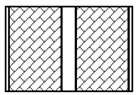
| South-West, North-West and North-East Walls | Layer Material | Thickness | Thermal Conductivity | Density | Specific Heat |
| Wall thickness 0.19 m, U-value = 0.54 W/m2K | (m) | (W/mK) | (kg/m3) | (J/kg K) | |
 | Bitumen | 0.004 | 0.2 | 1075 | 1000 |
| Steel | 0.0025 | 36 | 7700 | 500 | |
| Thermal insulation | 0.05 | 0.065 | 44 | 1458 | |
| Steel | 0.0025 | 36 | 7700 | 500 | |
| Thermal insulation | 0.05 | 0.065 | 44 | 1458 | |
| Autoclaved cellular concrete | 0.05 | 0.25 | 800 | 1000 | |
| Plaster | 0.015 | 0.2 | 1075 | 1000 | |
| South-East Wall | Material Layer | Thickness | Thermal Conductivity | Density | Specific Heat |
| Wall thickness 0.47 m, U-value = 0.57 W/m2K | (m) | (W/mK) | (kg/m3) | (J/kg K) | |
 | Plaster | 0.015 | 0.35 | 750 | 1000 |
| Semi-hollow brick | 0.20 | 0.32 | 1200 | 840 | |
| Air | 0.04 | 0.27 | 1.3 | 1008 | |
| Semi-hollow brick | 0.20 | 0.32 | 1200 | 840 | |
| Plaster | 0.015 | 0.35 | 750 | 1000 | |
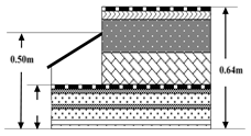
| Floor | Material Layer | Thickness | Thermal Conductivity | Density | Specific Heat |
| Wall thickness 0.48 m, U-value = 1.40 W/m2K | (m) | (W/mK) | (kg/m3) | (J/kg K) | |
 | Plaster | 0.015 | 0.35 | 750 | 1000 |
| Hollow block | 0.18 | 0.6 | 1400 | 840 | |
| Concrete slab | 0.20 | 1.6 | 2200 | 1000 | |
| Mortar bed | 0.05 | 0.9 | 1800 | 1000 | |
| Marble | 0.03 | 1.3 | 2300 | 840 | |
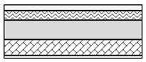
| Ceiling | Material Layer | Thickness | Thermal Conductivity | Density | Specific Heat |
| Average U-value = 0.16 W/m2K | (m) | (W/mK) | (kg/m3) | (J/kg K) | |
| Horizontal attic side | Bitumen | 0.02 | 0.20 | 1075 | 1000 |
| Mortar bed | 0.05 | 0.9 | 1800 | 1000 | |
| Concrete slab | 0.20 | 1.6 | 2200 | 1000 | |
| Hollow block | 0.18 | 0.6 | 1400 | 840 | |
| Tilted aluminum sheet side | Aluminum | 0.002 | 190 | 2700 | 900 |
| Polyurethane foam | 0.05 | 0.028 | 44 | 1458 | |
| Aluminum | 0.002 | 190 | 2700 | 900 | |
| Air | 0.1–0.3 | 0.27 | 1.3 | 1008 | |
 | Bitumen | 0.004 | 0.20 | 1075 | 1000 |
| Steel | 0.0025 | 36 | 7700 | 500 | |
| Thermal insulation | 0.06 | 0.028 | 44 | 1458 | |
| Steel | 0.0025 | 36 | 7700 | 500 | |
| Thermal insulation | 0.06 | 0.028 | 44 | 1458 | |
| Air | 0.04 | 0.27 | 1.3 | 1008 | |
| Plasterboard | 0.015 | 0.21 | 900 | 840 | |
| Case | αext (-) | αint (-) | LW (-) | LW (-) | ||
|---|---|---|---|---|---|---|
| Roof | Wall | Ceiling/Floor | Wall | Interior Surfaces | ||
| Reference (RC) | 0.6 | 0.3 | 0.25/0.5 | 0.25 | 0.1 | 0.9 |
| Low-Emissivity (LEC) | 0.15 | 0.9 | 0.1 | |||
| Cool Coating (CCC) | 0.33–0.6 (calculated by Equation (8)) | 0.15–0.3 (calculated by Equation (8)) | 0.25 | 0.1 | 0.9 | |
| Low-Emissivity and Cool Coating (LEC&CCC) | 0.15 | 0.9 | 0.1 | |||
© 2019 by the authors. Licensee MDPI, Basel, Switzerland. This article is an open access article distributed under the terms and conditions of the Creative Commons Attribution (CC BY) license (http://creativecommons.org/licenses/by/4.0/).
Share and Cite
Barone, G.; Buonomano, A.; Forzano, C.; Palombo, A. Building Energy Performance Analysis: An Experimental Validation of an In-House Dynamic Simulation Tool through a Real Test Room. Energies 2019, 12, 4107. https://doi.org/10.3390/en12214107
Barone G, Buonomano A, Forzano C, Palombo A. Building Energy Performance Analysis: An Experimental Validation of an In-House Dynamic Simulation Tool through a Real Test Room. Energies. 2019; 12(21):4107. https://doi.org/10.3390/en12214107
Chicago/Turabian StyleBarone, Giovanni, Annamaria Buonomano, Cesare Forzano, and Adolfo Palombo. 2019. "Building Energy Performance Analysis: An Experimental Validation of an In-House Dynamic Simulation Tool through a Real Test Room" Energies 12, no. 21: 4107. https://doi.org/10.3390/en12214107