Sensor Fault Tolerant Control for Aircraft Engines Using Sliding Mode Observer

Abstract

This paper investigated the problem of fault estimation and fault-tolerant control (FTC) against sensor faults for aircraft engines. By applying a second order sliding mode observer (SOSMO) to the engine on-board model, estimations of the system states and sensor faults could be obtained simultaneously, and the result of state estimation was unaffected when using the reduced-order sliding mode system. This result gave rise to the idea to use the estimated states instead of physical sensor signal in the engine close-loop feedback control. Unlike those using passive FTC concepts, the tradeoff between control performance and robustness was inherently unnecessary. Meanwhile, compared to active FTC approaches, because any classical state/output feedback method can be directly applied to the proposed scheme without any controller reconfiguration, extra undesired dynamic responses caused by parameter reconfiguring were avoided. In this paper, the proposed FTC scheme was tested on the nonlinear model of a civil aircraft turbofan engine, and numerical simulation results showed satisfactory sensor FTC performance.

1. Introduction

The increasing complexity of modern aircraft engines leads to a challenging task of handling malfunctions. As a result of the increasing demand for higher safety and reliability standards, the study of fault-tolerant control has received significant attention for modern aero-engine applications. The fault-tolerant control system can maintain desirable performance and stability properties in spite of the occurrence of faults. Generally speaking, fault-tolerant control can be classified into two types—passive and active scheme [1]. Passive scheme needs neither fault detection and identification (FDI) scheme nor reconfigurable controller, but is conservative because its application range is limited to the class of faults desired and considered in the design, making a trade-off between performance and robustness [2]. Active scheme maintains the stability and acceptable performance by reconfiguring controller with the fault information obtained by FDI system [3]. Although enormous work in the aerospace field is concerned with fault-tolerant control, most of the considered scenarios correspond to actuator faults. However, so far there has been limited work with respect to sensor fault tolerant control, especially for aero-engine applications. The main reason lies in that aircraft engine sensors are generally equipped with double or triple hardware redundancy, especially for those used in control loops. This allows the faulty sensors to be excluded from being used at the expense of increasing weight, which translates to higher fuel burn, higher carbon emission, and higher operating costs [4]. A feasible solution to this is to replace the extra set of hardware with analytical redundancy; thus, sensor fault-tolerant control (FTC) for aero-engine becomes a significant research field to be explored.

Recently FTC based on sliding mode techniques [5,6] has been active in fields of research, due to the robustness properties and fault reconstruction abilities. In particular, sliding mode observer (SMO) has been successfully incorporated within the observer-based fault estimation and FTC approaches, and it has been proven to be an effective way to estimate/reconstruct system faults and an appropriate basis of FTC design [7]. A sliding mode observer concerned with fault detection and isolation problem is proposed in [8], and faults are reconstructed by using the equivalent output error injection term during sliding motion. In most research papers, actuator faults are commonly considered. Tan utilized an appropriate filtering to yield an augmented system, in which sensor faults can be treated as actuator faults [9]. A generic FDI development in terms of reconstruction of faults using sliding mode observers is given by Tan and Edwards [10], and they extended the work in [8] for robust reconstruction of sensor and actuator faults by minimizing the effect of uncertainty on the reconstruction in an $ℒ2$ sense. Our previous work in [11,12] exploited the application of SMO in robust health estimation and sensor fault diagnosis for aircraft engines. The work in [13] described a sensor FTC scheme based on the SMO in [10]. The novelty lay in the application of the sensor fault reconstruction signal to correct the corrupted measured signals before being used by the controller and, therefore, the controller does not need to be reconfigured to adapt to sensor faults. The work in [14,15,16] implemented the work of [13] with the emphasis on reconstructing actuator/sensor faults and fault-tolerant control in a large civil aircraft using FTLAB747 software for implementation and testing. The scheme proposed in [13] was technically neither passive nor active —the sensor fault estimate information was used to correct the measured output signals, but not strictly in an active sense, as no adjustment or adaptation of the controller gains took place, which was more advanced and structure-simplified than traditional active FTC. However, in scenarios where a fault occurs with rapid shift, no matter how quick the SMO reacts, the convergence of sliding modes give rise to the undesirable system dynamics in corrected sensor signals, which may affect closed loop performance, for instance, causing overshooting in engine temperatures or pressures. Figure 1 summarizes the main existing work related to aircraft engine FDI and FTC based on sliding mode techniques.

This paper proposes a new scheme for aero-engine sensor fault FTC based on a sliding mode observer. On the basis of the results of [12], a second order sliding mode observer was constructed on an augmented filtered system. When sliding modes converged to sliding manifold, the estimation of states and faults could be both obtained, and the state estimation results were unaffected by sensor faults due to the reduced order manner. Unlike the work in [13] where fault reconstruction signal was employed to correct faulty sensors, in the proposed method, the related sensors were directly replaced with virtual state estimation signal; thus, undesired dynamic response caused by sensor signal reconfiguring was avoided. Additionally, in the proposed FTC architecture, the only new or additional component to the original control system was the sliding mode observer and it was easy to be retrofitted or combined with the existing controller to provide sensor FTC capability. The proposed FTC scheme was examined by a linear quadratic regulator (LQR), and numerical simulation results on the nonlinear model of a civil aircraft turbofan engine showed robust fault reconstruction and good sensor FTC performance.

2. Aircraft Engine Descriptions and Modeling

2.1. Engine Descriptions

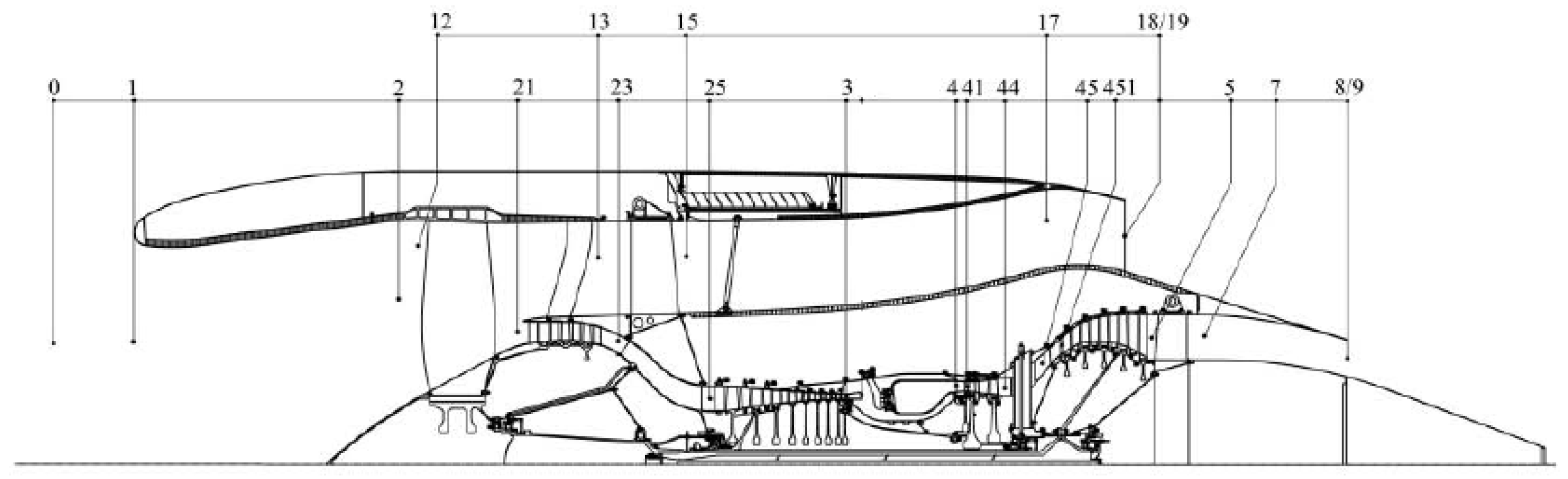
A high bypass twin spool mixing-exhaust turbofan engine was studied in this paper, of which the schematic description is shown in Figure 2. The airflow was supplied by a single inlet. Airflow passed through the fan and separated into two streams—one passed through engine core path, and the other passed through the bypass duct. Fuel was injected in the combustor and burned to produce the hot gas to drive the turbines. The fan and low pressure compressor (LPC) were driven by a low pressure turbine (LPT), whereas the high pressure compressor (HPC) was driven by a high pressure turbine (HPT). The airflow left through the nozzle. The notations used in this paper and their descriptions are shown in

Table 1. The notations and their descriptions.

Notation	Description
H	Height
Ma	Mach number
NL	Low pressure rotor speed
NH	High pressure rotor speed
Wf	Fuel flow rate
${\theta }_{\mathrm{VSV}}$	Variable stator vane angle
P25	High pressure compressor (HPC) inlet pressure
T25	HPC inlet temperature
P3	Combustor inlet pressure
T3	Combustor inlet temperature
T451	Exhaust gas temperature

.

Mechanical system dynamics due to rotating inertias constituted the most important contribution to engine transient behavior. Thus, rotating dynamics were the most important dynamics to be considered. In light of this, the state vector $\mathit{x}\in R^n$ was chosen as ${\left[N_L,N_H\right]}^{\mathrm{T}}$. Newton’s law for rotating masses was applied to each shaft as

$$\begin{array}{c}{\dot{N}}_L=f_1\left(N_{\mathit{L}},N_H,\mathit{u},\mathit{v}\right),\\ {\dot{N}}_H=f_2\left(N_{\mathit{L}},N_H,\mathit{u},\mathit{v}\right),\end{array}$$

(1)

where f₁ and f₂ are the net torques delivered by LPT and HPT. $\mathit{u}\in R^m$ is the control input and v denotes the external parameters (flight condition). Considering air flow mass, power, and momentum conservation laws, a general gas turbine simulation was designed using the concept in [17]. The engine design operation data and characteristic maps of rotating components such as fan, compressor, HPT, and LPT were loaded to the general simulation for obtaining a certain turbofan engine model [18]. The nonlinear model representing a turbofan engine was given by

$$\begin{array}{c}\dot{\mathit{x}}=f\left(\mathit{x},\mathit{u},\mathit{v}\right),\\ \mathit{y}=g\left(\mathit{x},\mathit{u},\mathit{v}\right),\end{array}$$

(2)

where $\mathit{y}\in R^p$ is the output. In the engine involved in this paper, the available sensors were $\mathit{y}={\left[N_L,N_H,P_{25},T_{25},P_3,T_3,T_{451}\right]}^{\mathrm{T}}.$ The function $f$ and $g$ are, respectively, the engine process and measurement expressions. The engine was coded with C language and packaged by Dynamic Link Library (DLL) for simulation in Matlab (2016a, MathWorks, Natick, MA, USA) environment [19]. Taylor approximation was applied to the engine model Equation (2) at the equilibrium point (${\mathit{x}}_0$, ${\mathit{u}}_0$), and retaining constant and first-order terms yielded the following state variable model (SVM):

$$\begin{array}{c}\dot{\mathit{x}}=f(\mathit{x},\mathit{u})\approx f({\mathit{x}}_0,{\mathit{u}}_0)+\frac{\partial f}{\partial \mathit{x}}|{}_{(x_0,u_0)}\Delta \mathit{x}+\frac{\partial f}{\partial \mathit{u}}|{}_{(x_0,u_0)}\Delta \mathit{u}\\ \mathit{y}=g(\mathit{x},\mathit{u})\approx g({\mathit{x}}_0,{\mathit{u}}_0)+\frac{\partial g}{\partial \mathit{x}}|{}_{(x_0,u_0)}\Delta \mathit{x}+\frac{\partial g}{\partial \mathit{u}}|{}_{(x_0,u_0)}\Delta \mathit{u}\end{array}$$

(3)

Equation (3) can be further depicted as

$$\begin{array}{l}\Delta \dot{\mathit{x}}=\mathit{A}\Delta \mathit{x}+\mathit{B}\Delta \mathit{u}\\ \Delta \mathit{y}=\mathit{C}\Delta \mathit{x}+\mathit{D}\Delta \mathit{u}\end{array}$$

(4)

where $\mathit{A}$, $\mathit{B}$, $\mathit{C}$, and $\mathit{D}$ are the system matrices with appropriate dimensions, and $\Delta \mathit{x}=\mathit{x}-{\mathit{x}}_0$, $\Delta \mathit{y}=\mathit{y}-{\mathit{y}}_0$, and $\Delta \mathit{u}=\mathit{u}-{\mathit{u}}_0$. For simplicity, the sign “$\Delta$” in Equation (4) was omitted in the following deductions. In addition, the quantities of different variables in Equation (4) were far away from each other. For instance, the normal physical quantity of $N_H$ at the design point was about 15,012 r/min, whereas the normal physical value of fuel flow $W_f$ at the design point was around 0.3606 kg/s. The large difference in the magnitudes of various model variables would lead to large difference of matrix singular values in the SVM, and it produced a big condition number of the system matrix. The larger the condition number was, the harder it was to compute a matrix inverse. Hence, physical operating parameters in the in-flight model were performed by parameter normalization, details referred in [18].

2.2. Hybrid Fitting Method for Linearization

The system matrices played an important role in the steady and transient performance of the SVM. There are commonly two ways to compute the system matrices, these being partial derivative method and fitting method. In the former method, partial derivative in the element of system matrices is computed by perturbing one state variable, and other state variables remain unchanged. However, in practice it is merely impossible that only one state changes while another remains unchanged by engine nature; thus, models solved by partial derivative method lack accuracy, especially during dynamic process. The fitting method generates the system matrices’ elements with the object function of least square errors between the component-level model (CLM) and model responses to step inputs. Choosing the perturbing amplitude and direction relies on the experiences—they closely affect to the SVM modeling accuracy. In addition, the curve part of step response data mainly depicts the system dynamics, and the remainder of the data shows the system steady behavior. Because the different part is processed in the same way, it is thus hard to address the steady and transient performance of the SVM at the same time.

In this paper, a hybrid fitting method was developed from the combination of partial perturbing and fitting methods. The matrices $\mathit{A}$ and $\mathit{C}$ were related to the transient stage, whereas the matrices $\mathit{B}$ and $\mathit{D}$ related to steady stage of step response. The initials of matrices $\mathit{A}$ and $\mathit{C}$ were obtained by the partial perturbing method, and steady-state component was used to compute the initials of matrices $\mathit{B}$ and $\mathit{D}$. The initials of matrices $\mathit{B}$ and $\mathit{D}$ were directly computed from the steady terminal values of one-control-variable step response by algebraic operation. The initials of these system matrices were acquired from the above implementations, and then the fitting method was employed to obtain the optimal system matrices, which follow the least square errors. The detailed procedure of the hybrid fitting approach is given as follows:

(1) By applying partial derivative method to calculate initial $\mathit{A}$ and $\mathit{C}$. Specifically, by imposing perturbation to each state variable, meanwhile other state variables and inputs remain unchanged, then corresponding coefficient in $\mathit{A}$ and $\mathit{C}$ can be calculated. Taking ${\mathit{N}}_L$ as an example, when perturbing ${\mathit{N}}_L$, let ${\mathit{N}}_H=0$ and ${\mathit{W}}_f=0$, then

$$\begin{array}{l}{\dot{N}}_L=a_{11}{N}_L+a_{12}{N}_H+b_{11}{W}_f\\ \Rightarrow a_{11}=\frac{{\dot{N}}_L}{N_L}\end{array}$$

(5)

(2) Using the step response of each input to yield the initial value of $\mathit{B}$ and $\mathit{D}$ A step of each input is injected to the nonlinear model, and using the steady terminal values of the step response data and initial $\mathit{A}$ and $\mathit{C}$, the initial value of $\mathit{B}$ and $\mathit{D}$ can be calculated. For example, injecting a 2% step in ${\mathit{W}}_f$, the elements of initial $\mathit{B}$ and $\mathit{D}$ is obtained by

$$\begin{array}{l}\left(\begin{array}{c}{b}_{11}\\ \begin{array}{l}{b}_{21}\\ \dots \\ b_{m1}\end{array}\end{array}\right)=-\left(\begin{array}{cc}{a}_{11}& a_{12}\\ a_{21}& a_{22}\\ \dots & \dots \\ a_{m1}& a_{m2}\end{array}\right)\left(\begin{array}{c}{N}_L\\ N_H\end{array}\right)/0.02\\ \left(\begin{array}{c}{d}_{11}\\ d_{21}\\ \dots \\ d_{p1}\end{array}\right)=\left(\begin{array}{c}{y}_{{}_{1,terminal}}\\ y_{{}_{2,terminal}}\\ \dots \\ y_{{}_{p,terminal}}\end{array}\right)/0.02-\left(\begin{array}{cc}{c}_{11}& c_{11}\\ c_{21}& c_{22}\\ \dots & \dots \\ c_{p1}& c_{p2}\end{array}\right)\left(\begin{array}{c}{N}_L\\ N_H\end{array}\right)/0.02\end{array}$$

(6)

(3) Use the initial $\mathit{A}$, $\mathit{B}$, $\mathit{C}$, and $\mathit{D}$ to create initial SVM. The same step input applied to nonlinear model is now imposed to the SVM, and the step response of SVM is obtained. In order to make the SVM output equal to the engine nonlinear model output in the steady state, the system matrices are tuned according to the output differences of the nonlinear model and SVM at equilibrium points by fitting method. When the demanded accuracy is reached, then $\mathit{A}$, $\mathit{B}$, $\mathit{C}$, and $\mathit{D}$ is the optimized solution.

It is noted that the calculation of matrices $\mathit{B}$ and $\mathit{D}$ elements depend on the matrices $\mathit{A}$ and $\mathit{C}$ at equilibrium points. The modeling data for the matrices $\mathit{A}$ and $\mathit{C}$ from perturbing one state variable to the nonlinear model cannot describe the engine dynamics well. Hence, the fitting method was used in this study to search the optimal $\mathit{A}$ and $\mathit{C}$ matrices with the aim of the least square output errors between the nonlinear model and SVM. The system matrices calculated from step (1) to step (2) were considered as the initials. The matrices $\mathit{B}$ and $\mathit{D}$ were calculated using the matrices $\mathit{A}$ and $\mathit{C}$ iterative optimization process from Equation (5) to Equation (6).

3. Sensor Fault Diagnosis

In this paper, the proposed sensor FTC was constructed on the basis of a second order sliding mode observer. This section describes the design of second order sliding mode observer (SOSMO) for sensor fault reconstruction and state estimation. At cruise operating point, the state variable model (SVM) of a commercial aircraft engine affected by sensor faults can be depicted by

$$\begin{array}{c}\dot{\mathit{x}}\left(t\right)=\mathit{A}\mathit{x}\left(t\right)+\mathit{B}\mathit{u}\left(t\right),\\ \mathit{y}\left(t\right)=\mathit{C}\mathit{x}\left(t\right)+\mathit{D}\mathit{u}\left(t\right)+\mathit{f}\left(t\right).\end{array}$$

(7)

As mentioned in last section, all variables considered in Equation (7) were normalized to [0, 1]. $\mathit{f}\left(\mathit{t}\right)={\left[f_1\left(t\right),f_2\left(t\right),\dots ,f_p\left(t\right)\right]}^{\mathrm{T}}$ denotes the unknown vector of sensor faults, where $f_i\left(t\right)\in \left[0,-1\right]$. $f_i\left(t\right)=0$ represents no fault in the $i$th sensor, and $f_i\left(t\right)=-1$ implies a total sensor failure, which was not considered in this paper, or otherwise the sensor is partially damaged. Assume $\mathit{f}\left(t\right)$ and its first-time derivatives are unknown but bounded

$$\Vert \mathit{f}\left(t\right)\Vert <{\alpha }_1,\Vert \dot{\mathit{f}}\left(t\right)\Vert <{\alpha }_2,$$

(8)

where ${\alpha }_1$, ${\alpha }_2$ are known real scalars. The notation $\Vert ·\Vert$ represents the Euclidean norm for vectors and the induced spectral norm for matrices.

Because fault reconstruction of actuators based on SMO has been widely studied as argued in [9], introducing a filter to the measurement equation is an effective way to make sensor faults be “treated” as actuators. On the basis of this idea, a new state $\mathit{z}\left(t\right)\in {ℝ}^p$, which is a filtered version of $\mathit{y}\left(t\right)$, given by

$$\dot{\mathit{z}}\left(t\right)=-{\mathit{A}}_f\mathit{z}\left(t\right)+{\mathit{A}}_f\mathit{y}\left(t\right)$$

(9)

where $-{\mathit{A}}_f\in {ℝ}^{p\times p}$ is Hurwitz. ${\mathit{A}}_f$ is typically in the form of a diagonal matrix, where the diagonal elements are positive and represent inverse time constants. Substituting $\mathit{z}\left(t\right)$ for $\mathit{y}\left(t\right)$ in Equation (1), the system is now described by

$$\begin{array}{c}\dot{\mathit{x}}\left(t\right)=\mathit{A}\mathit{x}\left(t\right)+\mathit{B}\mathit{u}\left(t\right),\\ \dot{\mathit{z}}\left(t\right)=-{\mathit{A}}_f\mathit{z}\left(t\right)+{\mathit{A}}_f\mathit{C}\mathit{x}\left(t\right)+{\mathit{A}}_f\mathit{D}\mathit{u}\left(t\right)+{\mathit{A}}_f\mathit{f}\left(t\right).\end{array}$$

(10)

In our previous work [12], the existence of a stable sliding motion toward Equation (10) was discussed, and it was proven that the necessary and sufficient conditions for building SOSMO were satisfied. Defining ${\mathit{e}}_z\left(t\right)=\widehat{\mathit{z}}\left(t\right)-\mathit{z}\left(t\right)$ as output estimation error, where $\widehat{\mathit{z}}\left(t\right)$ is the estimate value of $\mathit{z}\left(t\right)$, and the proposed SOSMO is constructed as follows

$$\begin{array}{c}\dot{\widehat{\mathit{x}}}\left(t\right)=\mathit{A}\widehat{\mathit{x}}\left(t\right)+\mathit{B}\mathit{u}\left(t\right),\\ \dot{\widehat{\mathit{z}}}\left(t\right)=-{\mathit{A}}_f\widehat{\mathit{z}}\left(t\right)+{\mathit{A}}_f\mathit{C}\widehat{\mathit{x}}\left(t\right)+{\mathit{A}}_f\mathit{D}\mathit{u}\left(t\right)+\mathit{\nu }\left(t\right)-\mathit{G}{\mathit{e}}_z\left(t\right),\end{array}$$

(11)

where $\widehat{\mathit{x}}\left(t\right)$ is the estimated value of $\mathit{x}\left(t\right)$, and $\mathit{G}\in {ℝ}^{p\times p}$ is the linear gain matrix to be designed. Defining ${\mathit{e}}_z\left(t\right)={\left[e_{z,1}\left(t\right),e_{z,2}\left(t\right),\dots ,e_{z,p}\left(t\right)\right]}^{\mathrm{T}}$, then $\mathit{\nu }\left(t\right)={\left[{\nu }_1\left(t\right),{\nu }_2\left(t\right),\dots ,{\nu }_p\left(t\right)\right]}^{\mathrm{T}}$ is defined component-wise as

$$\begin{array}{c}{\nu }_i\left(t\right)=-\psi sign\left(e_{z,i}\left(t\right)\right){\left|e_{z,i}\left(t\right)\right|}^{1/2}+d_i\left(t\right),\\ {\dot{d}}_i\left(t\right)=-\varsigma sign\left(e_{z,i}\left(t\right)\right)-\phi e_{z,i}\left(t\right) i=1,2,\dots ,p,\end{array}$$

(12)

where $\psi$, $\varsigma$, and $\phi$ are real scalars to be chosen. Define $\mathit{e}\left(t\right)=\widehat{\mathit{x}}\left(t\right)-\mathit{x}\left(t\right)$ as state estimation error. Let $\mathit{G}=-{\mathit{A}}_f+\chi {\mathit{I}}_p,$ where $\chi$ is a real scalar to be set, and ${\mathit{I}}_p\in {ℝ}^{p\times p}$ denotes identity matrix, then the error system can be written as

$$\begin{array}{c}{\dot{\mathit{e}}}_x\left(t\right)=\mathit{A}{\mathit{e}}_x\left(t\right),\\ {\dot{\mathit{e}}}_z\left(t\right)=-\chi {\mathit{I}}_p{\mathit{e}}_z\left(t\right)+{\mathit{A}}_f\mathit{C}{\mathit{e}}_x+\mathit{\nu }\left(t\right)-{\mathit{A}}_f\mathit{f}\left(t\right).\end{array}$$

(13)

The output error ${\mathit{e}}_z\left(t\right)$ is intended to be zero in finite time so that the state estimation and fault reconstruction can be accurate. Thus the sliding manifold is given by

$$S=\{{\left[\begin{array}{cc}{\mathit{e}}_x^{\mathrm{T}}\left(t\right)& {\mathit{e}}_z^{\mathrm{T}}\left(t\right)\end{array}\right]}^{\mathrm{T}}|{\mathit{e}}_z\left(t\right)=\mathbf{0}\}.$$

(14)

The objective is to let sliding mode ${\left[\begin{array}{cc}{\mathit{e}}_x^{\mathrm{T}}\left(t\right)& {\mathit{e}}_z^{\mathrm{T}}\left(t\right)\end{array}\right]}^{\mathrm{T}}$ be converged to the sliding manifold. Combining Equation (12) and Equation (13), the equation related to ${\dot{\mathit{e}}}_z\left(t\right)$ can be written component-wise as

$$\begin{array}{c}{\dot{e}}_{z,i}\left(t\right)=-\psi sign\left(e_{z,i}\left(t\right)\right){\left|e_{z,i}\left(t\right)\right|}^{1/2}-\chi e_{z,i}\left(t\right)+{\left({\mathit{A}}_f\mathit{C}\right)}_i{\mathit{e}}_x\left(t\right)-{\mathit{A}}_{f,i}\mathit{f}\left(t\right)+d_i\left(t\right),\\ {\dot{d}}_i\left(t\right)=-\varsigma sign\left(e_{z,i}\left(t\right)\right)-\phi e_{z,i}\left(t\right) i=1,2,\dots ,p,\end{array}$$

(15)

where ${\left({\mathit{A}}_f\mathit{C}\right)}_i$, ${\mathit{A}}_{f,i}$ represent the ith row of ${\mathit{A}}_f\mathit{C}$, ${\mathit{A}}_f$, respectively. For simplicity, a new variable $d_{0,i}$ ($i=1,2,\dots ,p$) is defined by

$$d_{0,i}\left(t\right)={\left({\mathit{A}}_f\mathit{C}\right)}_i{\mathit{e}}_x\left(t\right)-{\mathit{A}}_{f,i}\mathit{f}\left(t\right)+d_i\left(t\right) i=1,2,\dots ,p.$$

(16)

Substituting the related part in Equation (15) with Equation (16), then Equation (15) can be rewritten as

$$\begin{array}{c}{\dot{e}}_{z,i}\left(t\right)=-\psi sign\left(e_{z,i}\left(t\right)\right){\left|e_{z,i}\left(t\right)\right|}^{1/2}-\chi e_{z,i}\left(t\right)+d_{0,i}\left(t\right),\\ {\dot{d}}_{0,i}\left(t\right)=-\varsigma sign\left(e_{z,i}\left(t\right)\right)-\phi e_{z,i}\left(t\right)+{\varphi }_i\left(t\right) i=1,2,\dots ,p,\end{array}$$

(17)

where ${\varphi }_i\left(t\right)={\left({\mathit{A}}_f\mathit{C}\right)}_i{\dot{\mathit{e}}}_x\left(t\right)-{\mathit{A}}_{f,i}\dot{\mathit{f}}\left(t\right)$. Because $\mathit{A}$ is a stable matrix by engine nature, the equation associated with ${\mathit{e}}_x\left(t\right)$ in Equation (13) represents an autonomous error system and thereby is stable. Consequently, both $\Vert {\mathit{e}}_x\left(t\right)\Vert$ and $\Vert {\dot{\mathit{e}}}_x\left(t\right)\Vert$ are bounded. Provided $\Vert {\dot{\mathit{f}}}_1\left(t\right)\Vert$ are bounded, it is obvious that

$$\Vert {\varphi }_i\left(t\right)\Vert <\Vert {\left({\mathit{A}}_f\mathit{C}\right)}_i\Vert \Vert {\dot{\mathit{e}}}_x\left(t\right)\Vert +\Vert {\mathit{A}}_{f,i}\Vert \Vert \dot{\mathit{f}}\left(t\right)\Vert ,$$

(18)

which means there exists a sufficiently large $\epsilon$ with which ${\varphi }_i\left(t\right)<\epsilon$. As discussed in [19], Equation (17) is a special case of the super-twisting structure from [20]. The scalar gains from Equation (17) is set to satisfy the following conditions

$$\psi >2\sqrt{\epsilon },\chi >0,\varsigma >\epsilon ,\phi >\frac{{\chi }^2\left({\psi }^3+5/4{\psi }^2+5/2\left(\varsigma -\epsilon \right)\right)}{\psi \left(\varsigma -\epsilon \right)};$$

(19)

consequently, it can be proven that ${\dot{e}}_{z,i}\left(t\right)=e_{z,i}\left(t\right)=0$ in finite time [20], which means a sliding motion will take place.

During the sliding motion, ${\dot{e}}_{z,i}\left(t\right)=e_{z,i}\left(t\right)=0$, and the nonlinear signal $\mathit{\nu }$ must take on an average value to compensate for $\mathit{f}$ to maintain sliding. The average quantity, denoted by ${\mathit{\nu }}_{eq}$, is referred to as the equivalent output error injection term, which can be obtained from $\mathit{\nu }\left(t\right)$ by a low pass filter [21]. Once the sliding surface is reached, the error dynamics in Equation (13) are given by

$$\begin{array}{c}{\dot{\mathit{e}}}_x\left(t\right)=\mathit{A}{\mathit{e}}_x\left(t\right),\\ \mathit{0}={\mathit{A}}_f\mathit{C}{\mathit{e}}_x\left(t\right)+{\mathit{I}}_p{\mathit{\nu }}_{eq}\left(t\right)-{\mathit{A}}_f\mathit{f}\left(t\right).\end{array}$$

(20)

As mentioned, the system matrix $\mathit{A}$ is naturally stable, and the reduced-order error system is autonomous. Once converged, ${\mathit{e}}_x\left(t\right)$ is converged to zero, thus the estimated state vector $\widehat{\mathit{x}}$ is accurate. Meanwhile, the sensor fault reconstruction can be obtained from

$$\widehat{\mathit{f}}\left(t\right)={\mathit{A}}_f^{-1}{\mathit{\nu }}_{eq}\left(t\right).$$

(21)

In most state estimator designs, the output error is fed back to the state equation of the error system. However, when sensor fault occurs, the corrupted measurement signal would cause the estimated state to deviate. The uniqueness of the proposed observer lies in that the estimation of the system states is totally not affected by the occurrence of sensor faults. Because ${\mathit{e}}_z\left(t\right)$ and $\mathit{\nu }\left(t\right)$ are both imposed on the fictitious state $\mathit{z}\left(t\right)$ instead of ${\mathit{e}}_x\left(t\right)$, the derivative of ${\mathit{e}}_x\left(t\right)$ is by nature an autonomous system that would not be corrupted by sensor faults, and this feature can be explained by Equation (13) and Equation (20). Equation (13) and Equation (20) separately represent the error dynamics before and after the sliding surface being reached, and it can be seen that the derivatives of ${\mathit{e}}_x$ remain unchanged. In fact, the error system related to ${\mathit{e}}_x$ remains autonomous throughout the convergence of sliding motion, which is a critical merit when the observer is applied in the proposed FTC scheme in next section.

4. Fault Tolerant Control Based on State Estimation

In this section, the depicted sliding mode observer is integrated with the existing feedback controller to yield a sensor fault tolerant control scheme. Firstly the control plan of an aircraft engine is introduced. The chief task of an engine control system is to provide the proper amount of fuel to meet demanded thrust, which is not measurable. Fortunately, for a high by-pass ratio turbofan engine, low pressure rotor speed $N_L$ and thrust are highly correlated. $N_L$ is therefore widely used as a controlled variable for large civil aircraft engines. The output in Equation (7) is specified as $N_L$ in the following deductions. To meet the demand of command tracking in engine control loop, a tracking controller is feasible. That is, $N_L$ should catch up the command value reflected by throttle position in real-time. In order to induce the tracking error converged to 0, the derivative of the command deviation should be augmented into the state. Define $r$ as the command value of $y\left(t\right)$, then ${\mathit{e}}_r\left(t\right)=r\left(t\right)-y\left(t\right)$ is the command error vector. Corresponding to the system in Equation (1), take the derivative of ${\mathit{e}}_r\left(t\right)$:

$${\dot{\mathit{e}}}_r\left(t\right)=\frac{d\left(r\left(t\right)-y\left(t\right)\right)}{dt}=-\mathit{C}\dot{\mathit{x}}\left(t\right)-\mathit{D}\dot{\mathit{u}}\left(t\right).$$

(22)

Obviously, if ${\mathit{e}}_r$ is augmented into state vector, $\mathit{x}$ should be replaced with $\dot{\mathit{x}}\left(t\right)$ in the considered state equation. The augmented state turns to $\overline{\mathit{x}}\left(t\right)={\left[\begin{array}{cc}{\dot{\mathit{x}}}^{\mathrm{T}}\left(t\right)& {\mathit{e}}_r^{\mathrm{T}}\left(t\right)\end{array}\right]}^{\mathrm{T}}$, then the augmented state equation is obtained:

$$\dot{\overline{\mathit{x}}}\left(t\right)=\overline{\mathit{A}}\overline{\mathit{x}}\left(t\right)+\overline{\mathit{B}}\overline{\mathit{u}}\left(t\right)$$

(23)

where $\overline{\mathit{u}}\left(t\right)=\dot{\mathit{u}}\left(t\right)$, $\overline{\mathit{A}}=\left[\begin{array}{cc}\mathit{A}& \mathit{0}\\ -\mathit{C}& \mathit{0}\end{array}\right]$, and $\overline{\mathit{B}}=\left[\begin{array}{c}\mathit{B}\\ -\mathit{D}\end{array}\right]$. For such a tracking problem, some classical state feedback control methods can be effective and applicable. In this paper, an LQR controller is applied to the augmented plant. The quadratic performance index of system Equation (23) is

$$J={{\displaystyle \int }}_0^{\infty }\left({\mathit{x}}^{\mathrm{T}}\left(t\right)\mathit{Q}\mathit{x}\left(t\right)+{\mathit{u}}^{\mathrm{T}}\left(t\right)\mathit{R}\mathit{u}\left(t\right)\right)dt$$

(24)

where $\mathit{Q}\in {ℝ}^{n\times n}$ is a symmetric positive semi-definite matrix, and $\mathit{R}\in {ℝ}^{m\times m}$ is a symmetric positive definite matrix. By applying optimal control law

$${\overline{\mathit{u}}}^{*}\left(t\right)=-{\mathit{R}}^{-1}{\overline{\mathit{B}}}^T\mathit{P}{\overline{\mathit{x}}}^{*}\left(t\right)=-\overline{\mathit{K}}\overline{\mathit{x}}\left(t\right)$$

(25)

where $\mathit{P}$ is the symmetrically positive solution of an algebraic matrix Riccati equation, then the optimal $J$ is obtained with $J^{*}=\underset{\mathit{u}}{\min }J\left(\mathit{u}\left(t\right)\right)$. When $\mathit{Q}$ and $\mathit{R}$ are given, $\overline{\mathit{K}}$ can be calculated by solving $\mathit{P}$. Then

$$\overline{\mathit{u}}\left(t\right)=-\overline{\mathit{K}}\overline{\mathit{x}}\left(t\right)=-\left[\begin{array}{cc}{\mathit{K}}_{\dot{x}}& {\mathit{K}}_e\end{array}\right]\left[\begin{array}{c}\dot{\mathit{x}}\left(t\right)\\ {\mathit{e}}_r\left(t\right)\end{array}\right]$$

(26)

where ${\mathit{K}}_{\dot{x}}\in {ℝ}^{m\times n}$ and ${\mathit{K}}_e\in {ℝ}^{m\times p}$ are blocking controller gain matrices corresponding to $\dot{x}\left(t\right)$ and $e_r\left(t\right)$. Using Laplace transforms, the controller for original system is

$$\mathit{u}\left(t\right)=-{\mathit{K}}_{\dot{x}}\mathit{x}\left(t\right)-\frac{{\mathit{K}}_e{\mathit{e}}_r\left(t\right)}{s}.$$

(27)

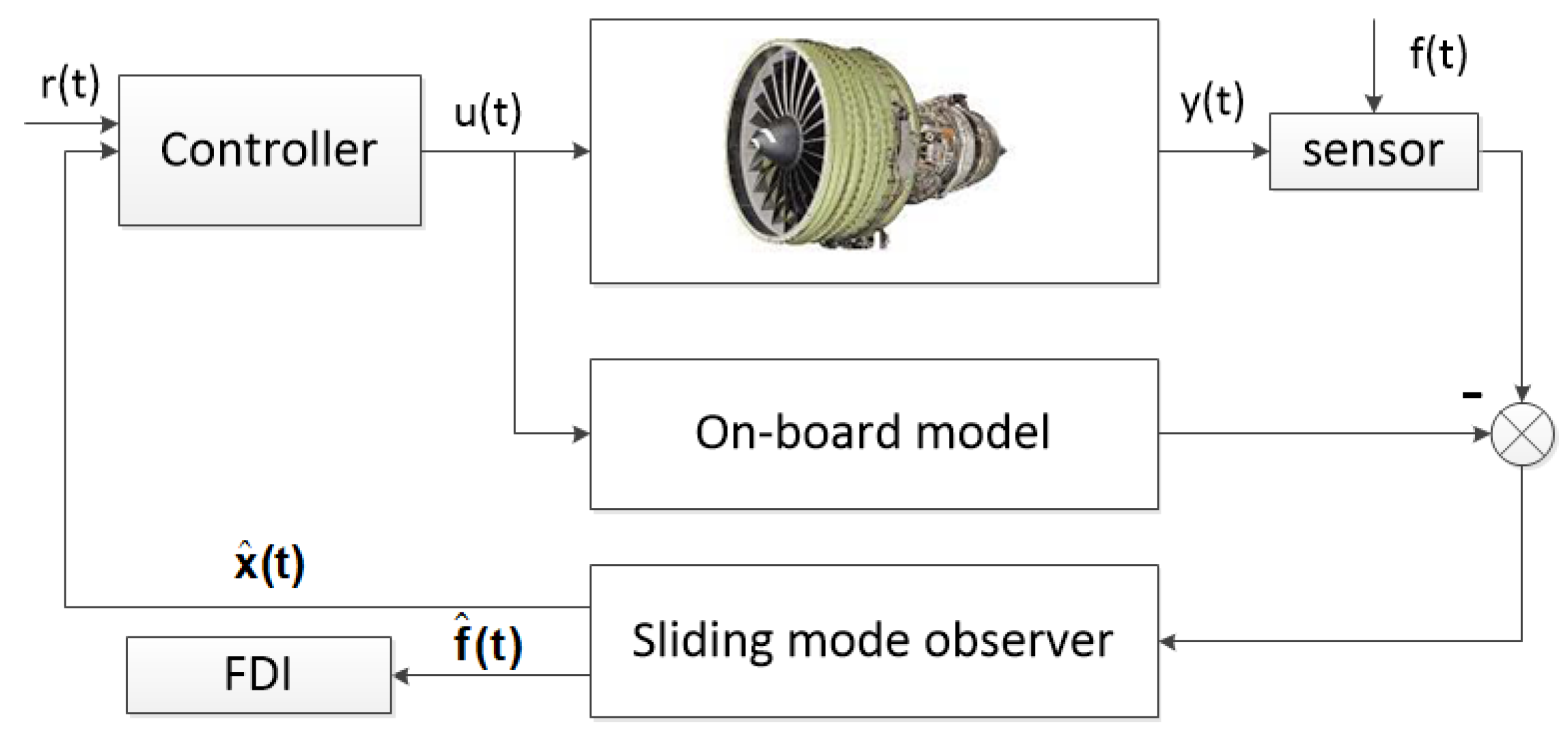
Because the rotor speeds of two shafts are both measurable, such a state feedback controller is feasible for engine control design. However, when sensor fault occurs, the deviation from corrupted sensor signal would cause the controller to react wrongly on command tracking. Many active sensor FTC schemes have been put forward, the common point of which is that they all reply on FDI results and parameter reconfigurations. Typical ideas include Kalman filters (KF) bank scheme, which is depicted in Figure 3. The KF bank, acting as a FDI part, detects and isolates the faulty sensor; then, a virtual sensor signal solved by KF is utilized to replace the damaged one. However, the efficiency of FTC relies much on the quality of FDI, and the sluggish manner of detection may bring about slow responses of FTC. Some researchers have used sliding mode theory to compensate for sensor faults, as shown in Figure 4. With the application of sliding mode observers, the sensor fault reconstruction signal can be obtained in real-time, and is employed to correct the corrupted measured signals before they are used by the controller. However in an abrupt fault case, the dynamics of reconstruction signal before the convergence of sliding mode may cause large overshooting in rotor speed, being even worse in fuel flow, which may lead to over temperature or over rotating problems.

The design observer discussed in the last sections is able to estimate state and sensor fault simultaneously, and sensor faults have no effect on ${\mathit{e}}_x\left(t\right)$. On the basis of this result, in this paper a new fault tolerant controller based on the described SOSMO was proposed, that is, the physical sensor signals for two shaft speeds are replaced with estimated value $\widehat{\mathit{x}}$ for state feedback, as shown in Figure 5. Because $\widehat{y}=\mathit{C}\widehat{\mathit{x}}+\mathit{D}\mathit{u}$, then

$${\dot{\widehat{\mathit{e}}}}_r\left(t\right)=\frac{d\left(r\left(t\right)-\widehat{y}\left(t\right)\right)}{dt}=-\mathit{C}\dot{\widehat{\mathit{x}}}\left(t\right)-\mathit{D}\dot{\mathit{u}}\left(t\right).$$

(28)

Considering the closed loop system

$$\dot{\overline{\mathit{x}}}\left(t\right)=\overline{\mathit{A}}\overline{\mathit{x}}\left(t\right)-\overline{\mathit{B}}\overline{\mathit{K}}\widehat{\overline{\mathit{x}}}\left(t\right)=\left(\overline{\mathit{A}}-\overline{\mathit{B}}\overline{\mathit{K}}\right)\overline{\mathit{x}}\left(t\right)-\overline{\mathit{B}}\overline{\mathit{K}}{\mathit{e}}_{\overline{x}}\left(t\right),$$

(29)

where

$${\mathit{e}}_{\overline{x}}\left(t\right)=\left[\begin{array}{c}\dot{\widehat{\mathit{x}}}\left(t\right)-\dot{\mathit{x}}\left(t\right)\\ {\widehat{\mathit{e}}}_r\left(t\right)-{\mathit{e}}_r\left(t\right)\end{array}\right]=\left[\begin{array}{c}{\dot{\mathit{e}}}_x\\ r-\mathit{C}\widehat{\mathit{x}}-\mathit{D}\mathit{u}-\left(r-\mathit{C}\mathit{x}-\mathit{D}\mathit{u}\right)\end{array}\right]=\left[\begin{array}{c}\mathit{A}{\mathit{e}}_x\\ -\mathit{C}{\mathit{e}}_x\end{array}\right],$$

(30)

where time variable $t$ is omitted for convenience. Thus the derivative of $\overline{\mathit{x}}$ is transformed to

$$\dot{\overline{\mathit{x}}}=\overline{\mathit{A}}\overline{\mathit{x}}-\overline{\mathit{B}}\overline{\mathit{K}}\widehat{\overline{\mathit{x}}}=\left(\overline{\mathit{A}}-\overline{\mathit{B}}\overline{\mathit{K}}\right)\overline{\mathit{x}}-\overline{\mathit{B}}{\mathit{K}}_{\dot{x}}\mathit{A}{\mathit{e}}_x+\overline{\mathit{B}}{\mathit{K}}_e\mathit{C}{\mathit{e}}_x.$$

(31)

Considering the result from Equation (20), the system associated with ${\mathit{e}}_x\left(t\right)$ is autonomous and unaffected by $\mathit{f}\left(t\right)$, then ${\left[\begin{array}{cc}{\overline{\mathit{x}}}^{\mathrm{T}}& {\mathit{e}}_x^{\mathrm{T}}\end{array}\right]}^{\mathrm{T}}$ is with the form

$$\left[\begin{array}{c}\dot{\overline{\mathit{x}}}\\ {\dot{\mathit{e}}}_x\end{array}\right]=\left[\begin{array}{cc}\overline{\mathit{A}}-\overline{\mathit{B}}\overline{\mathit{K}}& \overline{\mathit{B}}{\mathit{K}}_e\mathit{C}-\overline{\mathit{B}}{\mathit{K}}_{\dot{x}}\mathit{A}\\ \mathit{0}& \mathit{A}\end{array}\right]\left[\begin{array}{c}\overline{\mathit{x}}\\ {\mathit{e}}_x\end{array}\right]$$

(32)

which is a stable autonomous system. It is clear that the augmented system Equation (32) is not affected by sensor faults. It is essential the proposed observer can estimate $\mathit{x}\left(t\right)$ and reconstruct $\mathit{f}\left(t\right)$ simultaneously, which ensures the estimation of $\mathit{x}\left(t\right)$ is accurate without the corruption of $\mathit{f}\left(t\right)$.

5. Simulations

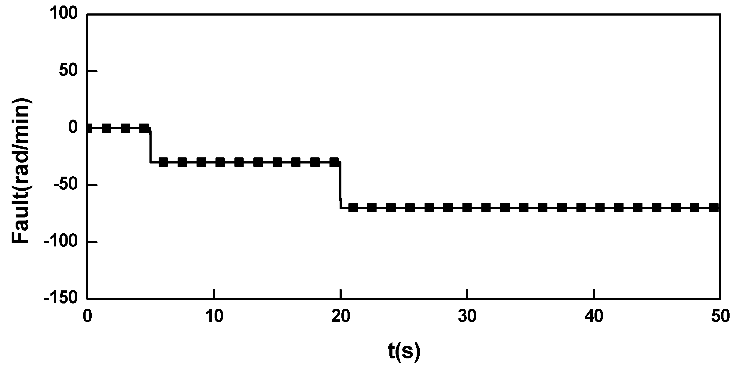
In this section, simulation results and performance evaluations of the proposed FTC scheme corresponding to sensor fault scenarios are presented. The same estimation tasks were implemented by the method in [13] to provide comparative results. Although the proposed FTC was based on a linear algorithm, tests were conducted via a nonlinear component-level model (CLM), which is a simulation platform representing a twin-spool high-bypass turbofan engine. The developed CLM was described in [18,22], and its fidelity has been proven against testing data extracted from real engines. The simulation environment was set to be at the reference flight condition and at a nominal cruise power setting, with $H=\mathrm{10,668}\mathrm{m}$, $M_{\mathrm{a}}=0.785$, $W_{\mathrm{f}}=0.3606 \mathrm{kg}/\mathrm{s}$, and ${\theta }_{\mathrm{VSV}}=0$. White Gaussian measurement noise and process noise were introduced to the experiments with standard deviations (percentage of the nominal value) ${\sigma }_{noise,m}=0.0015$ and ${\sigma }_{noise,p}=0.0005$, respectively, determined by practical experience and previously published data [22]. The considered sensor fault was imposed on $N_L$, as shown in Figure 6, which included two step faults separately occurring at 5 s (−0.86%) and 20 s (−2.02%) during simulations. Meanwhile, two steps in $N_L$ command, separately 1% at 10 s and −1% at 35 s, were imposed to examine the controller performance. Although in the algorithm design all variables were normalized, in the simulation the result variables were shown by their absolute values.

The matrices in SVM calculated by hybrid fitting method were given by

$$\begin{array}{c}\mathit{A}=\left[\begin{array}{cc}-1.299& 1.2841\\ -0.0549& -1.3196\end{array}\right], \mathit{B}=\left[\begin{array}{c}0.2253\\ 0.1884\end{array}\right],\\ \mathit{C}=\left[\begin{array}{c}\begin{array}{cc}1& 0\end{array}\\ \begin{array}{c}\begin{array}{cc}0& 1\end{array}\\ \begin{array}{c}\begin{array}{cc}0.3427& -0.1544\end{array}\\ \begin{array}{cc}1.0605& -0.5218\end{array}\\ \begin{array}{c}\begin{array}{cc}0.0534& 1.5177\end{array}\\ \begin{array}{cc}0.5819& 3.0115\end{array}\\ \begin{array}{cc}-0.3107& -0.9622\end{array}\end{array}\end{array}\end{array}\end{array}\right],\mathit{D}=\left[\begin{array}{c}0\\ 0\\ \begin{array}{c}0.0077\\ -0.0054\\ \begin{array}{c}0.00379\\ \begin{array}{c}0.1031\\ 0.5362\end{array}\end{array}\end{array}\end{array}\right].\end{array}$$

(33)

Aside from this, the related design parameter in sliding mode observer was given by $A_f=0.1I_7$, $\psi =0.11,$ $\chi =0.001,$ $\varsigma =0.013,$ $\phi =0.1$.

5.1. FTC Switched Off

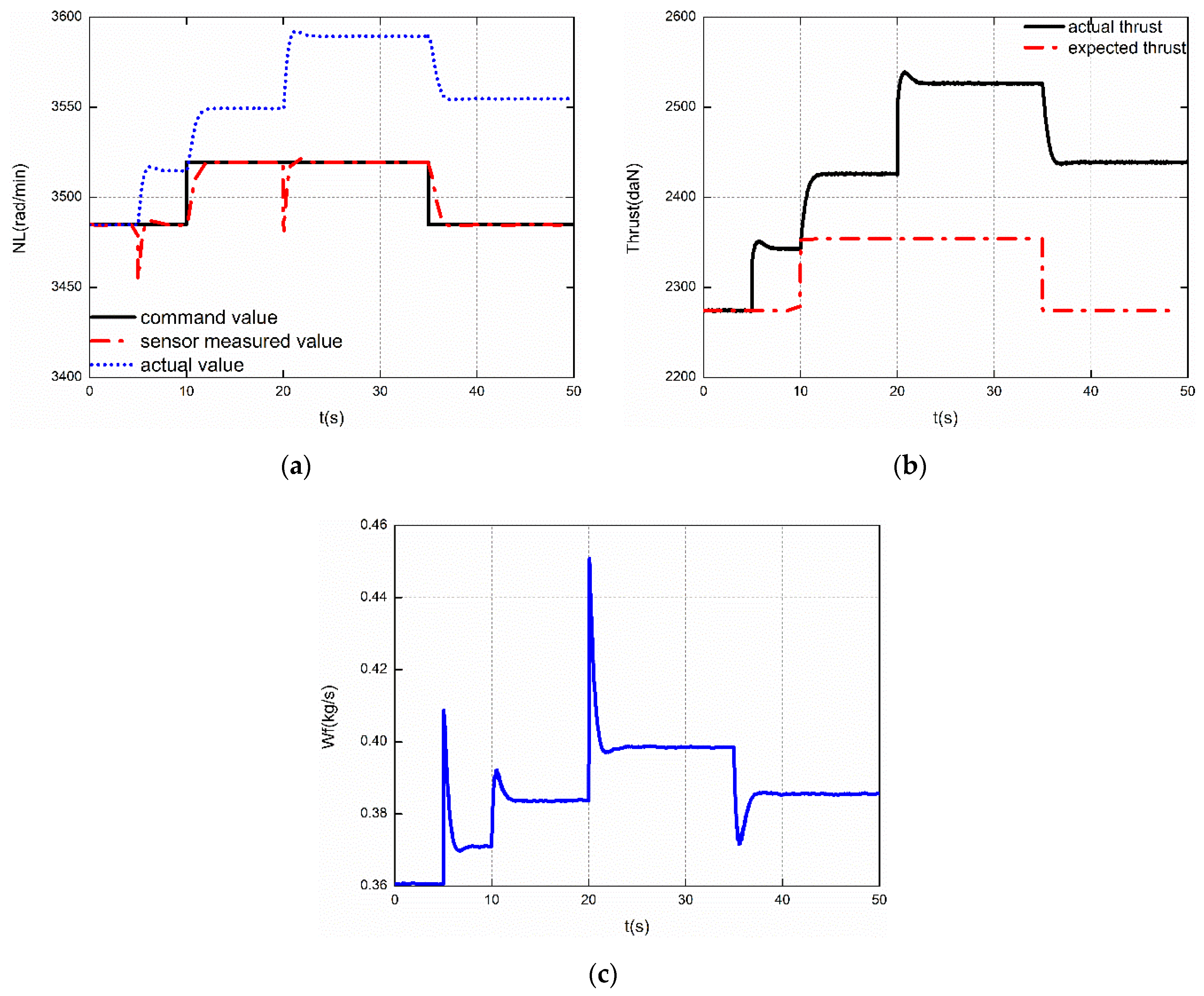
The designed tracking controller was initially examined without FTC scheme in the circumstance of sensor fault injections. Figure 7 shows the results when the corrupted signals (from faulty sensors) were directly used by the controller. Figure 7a shows the $N_L$ value regulated by LQR controller. Large deviations from the command value of $N_L$ could be observed, as shown by the blue line. By contrast, the corrupted sensor, denoted by the red line, tracked the command well. This indicated that the tracking controller worked normally, as the controller cannot “judge” if the sensor is faulty or not. However, the actual value of $N_L$ deviated from the command twice just at the instances where the step faults occurred. Figure 7b,c show the engine thrust and fuel flow, respectively, and they all diverged from the expected values due to the corrupted signal of the faulty sensor.

5.2. FTC by Compensation

Next, the FTC scheme proposed in [13] was applied to the control loop. The novelty of this method lies in its compatibility with any designed feedback control, and the corrupted sensor was mended with a reconstructed signal solved by SMO before being used in controller computations. Using the sliding mode observer depicted in Section 2, Figure 8a shows the sensor fault reconstruction results calculated by Equation (21), and the estimation error is shown in Figure 8b. It can be seen that the raw sensor fault was well reshaped, and the response of SMO was quick enough to catch the fault shifts. With the help of FTC, $N_L$ tracked the command well in sensor fault cases, as shown in Figure 8c. However, the value of $N_L$ fluctuated at the time when faults were imposed. This was because the steady state of the sliding mode was destroyed with the occurrence of faults, and the unexpected dynamics caused by the converging process was inevitable, which was reflected in the reconstructed signal and then the influence $N_L$ value and controller computing for fuel flow. At 5 s and 20 s, overshooting could be found in fuel flow and thrust, as shown in Figure 8d,e, which may cause over-temperature and over-rotating problems, even endangering flight safety.

5.3. FTC by State Estimation Feedback

The following are the results from the proposed FTC scheme that the measured state directly replaced with the estimated one. The same as the method in Section 5.2, the proposed scheme was compatible with any existing feedback controller without any controller reconfigurations. Figure 9a shows the state estimation results, and using the proper design of reduced-order sliding mode, the effects of sensor faults could be merely observed in estimated states. Figure 9b shows the $N_L$ result, where the blue line is the actual value used by controller computations and the red line is the value from the faulty sensor. Compared to Figure 8c, fluctuations caused by sensor faults were eliminated, and the $N_L$ command was nicely tracked. Meanwhile, overshooting in thrust or fuel flow occurred in last subsection; it was avoided here, which represents a major improvement over the prior method.

6. Conclusions

This paper proposed a sensor fault-tolerant control scheme for a high bypass turbofan engine based on sliding mode ideas. The proposed scheme was based on a second order sliding mode observer, by which the system state estimation and sensor fault reconstruction can be simultaneously obtained on-line. Meanwhile, due to the manner of reduced-order sliding mode, the state estimation was unaffected by sensor faults. The estimated states were then directly used to replace the physical corrupted sensor in the controller calculations, and therefore the controller does not need to be reconfigured, and unexpected overshooting caused by parameter tuning or FDI readjustment was avoided. The proposed scheme was implemented on the CLM of a commercial turbofan engine, and numerical simulation results showed its feasibility and improvement over traditional FTC.

References

- Patton, R.J. Robustness in model-based fault diagnosis: The 1997 situation. Annu. Rev. Control. 1997, 21, 101–121. [Google Scholar] [CrossRef]
- Blanke, M.; Kinnaert, M.; Lunze, J.; Staroswiechi, M. Diagnosis and Fault-Tolerant Control; Springer: Berlin, Germany, 2006. [Google Scholar]
- Hao, L.; Ying, Y.; Yong, Z.; Zhengen, Y. Active fault tolerant control with sliding mode observer. In Proceedings of the IEEE 34th Chinese Control Conference, Hangzhou, China, 28–30 July 2015; pp. 6259–6263. [Google Scholar]
- Goupil, P.; Marcos, A. Advanced Diagnosis for Sustainable Flight Guidance and Control. In Proceedings of the European ADDSAFE Project, SAE AeroTech Congress & Exhibition, Madrid, Spain, 31 March 2011. [Google Scholar]
- Utkin, V. Sliding Modes in Control Optimization; Springer: Berlin, Germany, 1992. [Google Scholar]
- Edwards, C.; Spurgeon, S.K. Sliding Mode Control: Theory and Applications; CRC Press: Boca Raton, FL, USA, 1998. [Google Scholar]
- Alwi, H.; Edwards, C.; Tan, C.P. Fault Detection and Fault-Tolerant Control Using Sliding Modes; Springer: Berlin, Germany, 2011. [Google Scholar]
- Edwards, C.; Spurgeon, S.K.; Patton, R.J. Sliding mode observers for fault detection and isolation. Automatica 2000, 36, 541–553. [Google Scholar] [CrossRef]
- Tan, C.P.; Edwards, C. Sliding mode observers for detection and reconstruction of sensor faults. Automatica 2002, 38, 1815–1821. [Google Scholar] [CrossRef]
- Tan, C.P.; Edwards, C. Sliding mode observers for robust detection and reconstruction of actuator and sensor faults. Int. J. Robust Nonlinear Control 2003, 13, 443–463. [Google Scholar] [CrossRef]
- Changm, X.; Huangm, J.; Lu, F. Health Parameter Estimation with Second-Order Sliding Mode Observer for a Turbofan Engine. Energies 2017, 10, 1040. [Google Scholar] [CrossRef]
- Chang, X.; Huang, J.; Lu, F. Robust In-Flight Sensor Fault Diagnostics for Aircraft Engine Based on Sliding Mode Observers. Sensors 2017, 17, 835. [Google Scholar] [CrossRef] [PubMed]
- Chen, L.; Alwi, H.; Edwards, C. Integrated LPV controller/estimator scheme using sliding modes. In Proceedings of the IEEE Conference on Decision and Control, Osaka, Japan, 15–18 December 2015; pp. 5124–5129. [Google Scholar]
- Alwi, H.; Edwards, C. Robust sensor fault estimation for tolerant control of a civil aircraft using sliding modes. In Proceedings of the IEEE American Control Conference, Minneapolis, MN, USA, 14–16 June 2006; p. 6. [Google Scholar]
- Alwi, H.; Edwards, C. Fault Detection and Fault-Tolerant Control of a Civil Aircraft Using a Sliding-Mode-Based Scheme. IEEE Transact. Control Syst. Technol. 2008, 16, 499–510. [Google Scholar] [CrossRef] [Green Version]
- Alwi, H.; Edwards, C. Sensor Fault Tolerant Control Using Sliding Mode Fault Reconstruction on an Aircraft Benchmark. In Proceedings of the AIAA Guidance, Navigation, and Control Conference, Minneapolis, MN, USA, 13–16 August 2013; pp. 143–155. [Google Scholar]
- Sugiyama, N. Derivation of system matrices from nonlinear dynamic simulation of jet engines. J. Guid. Control Dyn. 1994, 17, 1320–1326. [Google Scholar] [CrossRef]
- Zhou, W.X. Research on Object-Oriented Modeling and Simulation for Aero-engine and Control System. Ph.D. Thesis, Nanjing University of Aeronautics and Astronautics, Nanjing, China, 2006. (In Chinese). [Google Scholar]
- Alwi, H.; Edwards, C. Robust fault reconstruction for linear parameter varying systems using sliding mode observers. Int. J. Robust Nonlinear Control. 2013, 24, 1947–1968. [Google Scholar] [CrossRef] [Green Version]
- Moreno, J.A.; Osorio, M. Strict Lyapunov Functions for the Super-Twisting Algorithm. IEEE Trans. Autom. Control 2012, 57, 1035–1040. [Google Scholar] [CrossRef]
- Edwards, C.; Alwi, H.; Tan, C.P. Sliding Modes for Fault Detection and Fault-Tolerant Control. In Sliding Modes after the First Decade of the 21st Century; Springer: Berlin, Germany, 2012; pp. 293–323. [Google Scholar]
- Lu, F.; Huang, J.; Lv, Y. Gas Path Health Monitoring for a Turbofan Engine Based on a Nonlinear Filtering Approach. Energies 2013, 6, 492–513. [Google Scholar] [CrossRef] [Green Version]
Figure 1.
The main existing work related to aircraft engine fault detection and identification (FDI) and fault-tolerant control (FTC) based on sliding mode observer (SMO).
Figure 2.
Schematic description of two-spool turbofan engine.
Figure 3.
Schematic of FTC based on Kalman filters (KF) bank.
Figure 4.
Schematic of FTC based on fault reconstruction of sliding mode observer (SMO).
Figure 5.
Schematic of FTC based on state estimation of SMO.
Figure 6.
The sensor fault injection on .
Figure 7.
FTC switched off: (a) ; (b) thrust; (c) fuel flow.
Figure 8.
FTC by compensation: (a) sensor fault reconstruction; (b). estimation error; (c) ; (d) thrust; (e) fuel flow.
Figure 9.
FTC by state estimation feedback: (a) state estimation; (b) ; (c) thrust; (d). fuel flow.