Determinants of the Long-Term Correlation between Crude Oil and Stock Markets

Abstract

This study employed a dynamic conditional correlation–mixed-data sampling (DCC–MIDAS) approach and panel data analysis to examine the factors that influence the long-term correlation between crude oil and stock markets. Our study shows that there is a positive long-term conditional correlation between oil prices and stock markets, except during the 2008 global financial crisis and the 2011 European debt crisis. We also found that macroeconomic factors have a significant impact on this correlation. Specifically, risk-free rate has a positive effect, whereas economic activity and credit risk has a negative effect. Our results provide useful information for investors and monetary authorities.

1. Introduction

Studies on the co-movement between crude oil and stock markets have important implications for the formulation of energy policies and portfolio diversification. As one of the most important inputs in industrial production, crude oil significantly influences general price levels as well as economic activity. In the financial economic realm, the risk premium has a significant impact on the asset price of both crude oil and stock prices; for example, credit risk, interest rate, and volatility. As suggested by Hamilton [1], there has been a growing interest in the effects of oil prices on stock returns and the economy. In this paper, we mainly address the question of which kinds of factors can affect the co-movement between crude oil and stock markets. Understanding these factors will provide the additional information that is needed for portfolio diversification and policy-making. The time-varying correlation has been well documented (Malik and Hammoudeh [2]; Filis et al. [3]; Arouri et al. [4]; Tamakoshi and Hamori [5,6]; Basher and Sadorsky [7]) as a risk management tool in portfolio administration. Moreover, the financialization of the commodity markets is strengthening due to their strong correlation with other financial markets, especially stock markets. There is empirical evidence of a growing correlation between oil and stock markets (Büyüksahin and Robe [8]; Silvennoinen and Thorp [9]). Hence, there is good reason to investigate the factors affecting this correlation. Thus, we employed the dynamic conditional correlation–mixed-data sampling (DCC–MIDAS) model proposed by Colacito et al. [10] to define this long-term correlation. By utilizing the DCC–MIDAS method and panel data analysis, we could uncover the factors that influence the correlation in the long-term.

By adding crude oil to the portfolio as an alternative financial asset, we obtained an additional diversification benefit from its low correlation with the stock-based portfolio. Moreover, the co-movement of cross-assets has significant economic implications for the linkage between crude oil and stock markets, as the price of crude oil is a fundamental economic indicator. In particular, understanding the co-movement between stocks and crude oil markets in the long-term yields information about potential drivers to predict the future economy and hedge portfolio risks.

We provide useful information to investors regarding portfolio allocation or international diversification. This correlation is the key to achieving an optimal portfolio because changes in the correlation imply changes in portfolio weights. Specifically, our results indicate that macroeconomic factors work effectively in determining the correlation between oil and stock markets. Moreover, crude oil can reduce portfolio risk during a financial crisis when the correlation decreases.

Many extensive empirical studies have discussed the relationship between stocks and the stock market extensively. Generally, three types of studies can be categorized: the first type analyzes the causal relationship between stock and crude oil markets. Some studies have shown that stock market returns are significantly influenced by crude oil price movements (Aloui and Jammazi [11]; Chen [12]; Ghouri [13]; Jones and Kaul [14]; Kilian and Park [15]; Miller and Ratti [16]; Sadorsky [17]; Papapetrou [18]). These studies provided evidence of a negative effect on stock markets from a positive oil shock, although they employed different samples and consider different countries. On the other hand, other studies indicated that the relationship between the crude oil market and stock market is positive and significant. For example, Chen et al. [19], El-Sharif et al. [20], and Narayan and Narayan [21] provided evidence of a positive impact on the oil and gas sectors’ stock returns in the UK, given an increase in oil prices. In addition, other papers have provided similar evidence in developing countries (Kanjilal and Ghosh [2]; Li et al., [22]; Narayan and Narayan [21]; Zhu et al. [23]). By contrast, some of the literature has focused on the non-linear relationship between crude oil and the stock market (Narayan and Gupta [24]; Jiménez-Rodríguez [25]; Ponka [26]). Although their findings are mixed, crude oil still exhibits significant power on the stock market.

In contrast to the first type of study, the second type can be classified as investigating the dynamic correlation between stock and crude oil markets. Generally, the multivariate generalized autoregressive conditional heteroskedasticity (MGARCH) model has been applied in the energy finance literature (Arouri et al. [27,28]; Arouri et al. [4]; Basher and Sadorsky [7]; Conrad et al. [29]; Filis et al. [3]; Malik and Hammoudeh [30]; Malik and Ewing [31]; Sadorsky [32,33]). These studies mainly discussed the spillover effect and volatility transmission between stock and crude oil markets. For example, Filis et al. [3] provided evidence that the time-varying correlations between stocks and oil prices are similar for both oil-importing and oil-exporting countries. However, there is a bidirectional spillover effect between the US stock and crude oil market and a spillover effect from oil to European stock markets (Arouri et al. [4]; Arouri et al. [27]). As shown in the study of Conrad et al. [29], macroeconomic leading indicators will be helpful predictors of the oil–stock correlation. Basher and Sadorsky [7] provided an overview of the time-varying correlation between emerging stock and crude oil markets and estimated the hedging ratio. Bampinas and Panagiotidis [34] also summarized the time-varying cross-market linkage by considering the four major crises and found that oil can be an alternative safe haven asset during crises. Yin [35] and Nguyen and Walther [36] also found that the crude oil price responds to the macroeconomic condition sensitively in the framework of GARCH–MIDAS. Kilian [37] and Kilian [38] reported that the global real economic activity is an important driver for oil prices.

The third type of study includes other models which are employed to investigate the interdependence between stocks and oil. In most cases, this type of investigation is based on the copula model or wavelet analysis. For example, Aloui et al. [39] provided evidence of a positive dependence between oil and the stock markets in six Central and Eastern European countries. By employing the wavelet approach, Martín-Barragán et al. [40] found several correlational breakdowns caused by financial and oil shocks, both at lower and higher frequencies. Aloui and Aïssa [41] also provided evidence that the dynamics between stocks and oil prices are not constant over time, and the dependence structure of this was significantly affected by the 2007–2009 financial crisis. Cai et al. [42] analyzed the interdependence between oil and East Asian stock returns using wavelet techniques.

In summary, while numerous studies have explored the interdependence between crude oil and stock markets and volatility spillovers, little is known about the factors determining the long-term correlation between these two variables. The contribution of this study is threefold. First, we elicit detailed information from the volatility in stock and crude oil markets in both the short and long terms. As speculators are more interested in short-term investment, our study provides useful information to speculators and investors regarding hedging or portfolio management. Furthermore, the long-term co-movement between stocks and crude oil may provide an anchor for policymakers to implement economic policy. Secondly, we revealed detailed information about the time-varying correlation between stock and crude oil markets on both short- and long-term scales. Thus, we could detect dynamic structures and changes over various time periods and provide additional information regarding structural breaks in markets and economies. Specifically, instant changes in the market can be detected via short-term scales, while economic structural breaks can be identified by long-term scales. Finally, we comprehensively revealed the factors that can influence the co-movement between stock and crude oil markets. Particularly, by treating macroeconomic and financial factors differently, we could distinguish the influence of each factor, which provided us with a more detailed framework of the determinants of co-movement between stock and crude oil markets.

The rest of this paper is presented as follows. Section 2 analyzes the data based on the GARCH–MIDAS model. Section 3 identifies the factors that influence the dynamic correlation between the stock and crude oil markets in the long-term. Section 4 provides concluding remarks.

2. DCC–MIDAS Approach

2.1. GARCH–MIDAS Component Model

Following the studies of Colacito et al. [10], we summarized the DCC–MIDAS models and their empirical results in this section. (The DCC model itself was developed by Engle [43]. Also see Conrad et al. [29] and Yang et al. [44]). Suppose the vector of $n$ assets’ returns ${\mathit{r}}_{\mathit{t}}={\left(r_{1,t},r_{2,t},\cdots ,r_{n,t}\right)}^{\prime }$, follows ${\mathit{r}}_{\mathit{t}}\sim i.i.d.N\left(\mathit{\mu },{\mathit{H}}_{\mathit{t}}\right)$, where $i$ indicates each asset, $t$ indicates the day, $\mathit{\mu }$ denotes the vector of unconditional means, ${\mathit{H}}_{\mathit{t}}$ denotes the matrix of conditional covariance, and ${\mathit{D}}_{\mathit{t}}$ denotes a diagonal matrix of standard deviations; that is, ${\mathit{H}}_{\mathit{t}}={\mathit{D}}_{\mathit{t}}{\mathit{R}}_{\mathit{t}}{\mathit{D}}_{\mathit{t}}$ and ${\mathit{R}}_{\mathit{t}}=E_{t-1}\left[{\mathit{\xi }}_{\mathit{t}}{\mathit{\xi }}_{\mathit{t}}^{\mathbf{\prime }}\right]$, where ${\mathit{\xi }}_{\mathit{t}}={\mathit{D}}_{\mathit{t}}^{\mathbf{-}\mathbf{1}}\left({\mathit{r}}_{\mathit{t}}-\mathit{\mu }\right)$. The conditional volatilities ${\mathit{D}}_{\mathit{t}}$ and the conditional correlation matrix ${\mathit{R}}_{\mathit{t}}$ are estimated step-by-step, accordingly.

Following Engle et al.’s [45] GARCH–MIDAS model, we separate the volatility of each variable into long- and short-term components. Similarly, we employ the mean reverting daily GARCH process to estimate the GARCH–MIDAS model (Engle and Rangel [46]). Therefore, the GARCH–MIDAS process for each asset return $r_{i,t}$, $i=1,2,\cdots ,n$ is as follows:

$$r_{i,t}={\mu }_i+\sqrt{m_{i,\tau }·g_{i,t}}{\xi }_{i,t},\forall t=\left(\tau -1\right)N+1,\dots ,\tau N,\forall \tau =1,\dots ,T.$$

(1)

where $N_v$ denotes the trading days of one month and $\tau =1,\dots ,T$ signifies each month. We set $N_v=21.$ We assume that the short-run variance $g_{i,t}$ follows a simple mean reverting GARCH (1,1) process:

$$g_{i,t}=\left(1-{\alpha }_i-{\beta }_i\right)+{\alpha }_i\frac{{\left(r_{i,t-1}-{\mu }_i\right)}^2}{m_{i,\tau }}+{\beta }_i{g}_{i,t-1},{\alpha }_i>0,{\beta }_i\ge 0\mathrm{and}{\alpha }_i+{\beta }_i<1$$

(2)

The short-run variance $g_{i,t}$ is measured daily. In addition, a weighted sum of $K_v^i$ lags of realized variances ($RV$) over a long horizon is given by a low-frequency mixed-data sampling (MIDAS) component $m_{i,\tau }$ as follows:

$$m_{i,\tau }={\overline{m}}_i+{\theta }_i{\sum }_{l=1}^{K_v^i}{\phi }_l\left({\omega }_v^i\right)R{V}_{i,\tau }$$

(3)

$$R{V}_{i,\tau }={\sum }_{j=\left(\tau -1\right)N_v+1}^{\tau N_v}{\left(r_{i,j}\right)}^2$$

(4)

where τ denotes the time span, which is set at one month. To guarantee that the covariance is a stationary process with positive variance, the restriction conditions ${\overline{m}}_i>0$ and $0<{\theta }_i<1$ must be satisfied for the parameters ${\overline{m}}_i$ and ${\theta }_i$. The secular component $m_{i,\tau }$ contains information on the effect of expected global/macroeconomic variances on volatility, while the realized variance involves $N_v$ daily squared returns.

The beta weights in Equation (3) are defined as follows:

$${\phi }_l\left({\omega }_v^i\right)=\frac{{\left(1-l/K_v^i\right)}^{{\omega }_v^i-1}}{{\sum }_{j=1}^{K_v^i}{\left(1-j/K_v^i\right)}^{{\omega }_v^i-1}},$$

(5)

where the weight of past-realized variances is determined by parameters ${\omega }_v^i$ and $K_v^i$. In addition, the pattern of decay is ensured by the weighting scheme ${\phi }_l({\omega }_v^i)$, while the size of ${\omega }_v^i$ among the different series determines the rate of decay; that is, a larger ${\omega }_v^i$ indicates a pattern of a higher rate of decay. Following Colacito et al. [10], we assume that the parameters $K_v^i$, and ${\omega }_v^i$ remain the same across all series and are independent of i; that is, $K_v^i=K_v=36$, and ${\omega }_v^i={\omega }_v$.

2.2. DCC–MIDAS Models

To investigate the factors influencing the dynamic conditional correlation (DCC) between oil price and stock price in both the short and long term, we follow Engle and Rangel [46] by incorporating the MIDAS polynomial into the GARCH and DCC model. Therefore, we construct the matrix ${\mathit{Q}}_{\mathit{t}}$ to calculate dynamic correlations through volatility-adjusted (standardized) residuals ${\xi }_{i,t}$ as follows:

$${\mathit{Q}}_{\mathit{t}}=\left(1-a-b\right){\overline{\mathit{R}}}_{\mathit{t}}+a{\mathit{\xi }}_{\mathit{t}\mathbf{-}\mathbf{1}}{\mathit{\xi }}_{\mathit{t}\mathbf{-}\mathbf{1}}^{\mathbf{\prime }}+b{\mathit{Q}}_{\mathit{t}\mathbf{-}\mathbf{1}},$$

(6)

where ${\mathit{Q}}_{\mathit{t}}$ denotes an approximate conditional correlation. To satisfy stationary conditions, parameters a and b must be greater than 0 and their sum must be less than 1. The conditional correlation matrix $diag{\left\{{\mathit{Q}}_{\mathit{t}}\right\}}^{-\frac{1}{2}}{\mathit{Q}}_{\mathit{t}}diag{\left\{{\mathit{Q}}_{\mathit{t}}\right\}}^{-\frac{1}{2}}$ is used to obtain ${\mathit{R}}_{\mathit{t}}$.

The elements $q_{i,j,t}$ in $Q_t$ in Equation (6) are expressed by

$$q_{i,j,t}={\overline{\rho }}_{i,j,t}\left(1-a-b\right)+a{\xi }_{i,t-1}{\xi }_{j,t-1}+b{q}_{i,j,t-1},$$

(7)

$${\overline{\rho }}_{i,j,t}={\sum }_{l=1}^{K_c^{ij}}{\phi }_{\mathrm{l}}\left({\omega }_r^{ij}\right)c_{i,j,t-\mathrm{l}},$$

(8)

$$c_{i,j,t}=\frac{{\sum }_{k=t-N_c^{ij}}^t{\xi }_{i,k}{\xi }_{j,k}}{\sqrt{{\sum }_{k=t-N_c^{ij}}^t{\xi }_{i,k}^2}\sqrt{{\sum }_{k=t-N_c^{ij}}^t{\xi }_{j,k}^2}},$$

(9)

where the weighting scheme is similar to Equation (5). Specifically, the short-term covariance is described by $q_{i,j,t}$. The short-term correlation is described by ${\rho }_{i,j,t}$; that is, ${\rho }_{i,j,y}=q_{i,j,t}/\sqrt{q_{i,i,t}}\sqrt{q_{j,j,t}}$. The long-term correlation is described by ${\overline{\rho }}_{i,j,t}$. Thus, Equation (7) can be rewritten as

$$q_{i,j,t}-{\overline{\rho }}_{i,j,t}=a\left({\xi }_{i,t-1}{\xi }_{j,t-1}-{\overline{\rho }}_{i,j,t}\right)+b\left(q_{i,j,t-1}-{\overline{\rho }}_{i,j,t}\right).$$

(10)

Equation (10) can be interpreted as the fluctuations of a daily correlation in a monthly correlation, which are different from the structure of the GARCH–MIDAS regarding the two components of volatility; that is, the classic dynamic correlation’s autoregressive structure is modeled using the short-run variations in covariance ($q_{i,j,t}$), while the secular or fundamental origins of time variations in correlation are modeled by the long-run component (${\overline{\rho }}_{i,j,t}$), which is denoted as ${\mathrm{cc}}_{i,\tau }$ in the following regression. Following Colacito et al. [10], we assume that the weights (${\omega }_r^{ij}$), lag length ($N_c^{ij}$ = 21), and span length of historical correlation ($K_c^{ij}$ = 144) are common to all series pairs in Equations (7)–(9).

2.3. Estimation Method

Here, we employ a two-step procedure to estimate all the parameters of the model. Initially, we employ vector $\Psi =\left({\alpha }_i,{\beta }_i,{\omega }_i,m_i,{\theta }_i;i=1,2,\dots n\right)$ to estimate the parameters of the univariate conditional volatility models. Then, we employ vector $\Xi =\left(a,b,{\omega }_r\right)$ to estimate the conditional correlation model’s parameters. Hence, by maximizing the following quasi-likelihood function (Equations (11)–(13)), we obtain the estimate of each parameter.

$$QL\left(\Psi ,\Xi \right)=Q{L}_1(\Psi )+Q{L}_2\left(\Psi ,\Xi \right),$$

(11)

$$Q{L}_1(\Psi )=-{\sum }_{t=1}^T\left(nlog\left(2\pi \right)+2\log \left(\left|{\mathit{D}}_{\mathit{t}}\right|\right)+{\mathit{r}}_{\mathit{t}}^{\mathbf{\prime }}{\mathit{D}}_{\mathit{t}}^{\mathbf{-}\mathbf{2}}{\mathit{r}}_{\mathit{t}}\right),$$

(12)

$$Q{L}_2\left(\Psi ,\Xi \right)=-{\sum }_{t=1}^T\left(log\left(\left|{\mathit{R}}_{\mathit{t}}\right|\right)+{\mathit{\xi }}_{\mathit{t}}^{\mathbf{\prime }}{\mathit{R}}_{\mathit{t}}^{\mathbf{-}\mathbf{1}}{\mathit{\xi }}_{\mathit{t}}+{\mathit{\xi }}_{\mathit{t}}^{\mathbf{\prime }}{\mathit{\xi }}_{\mathit{t}}\right).$$

(13)

2.4. Data

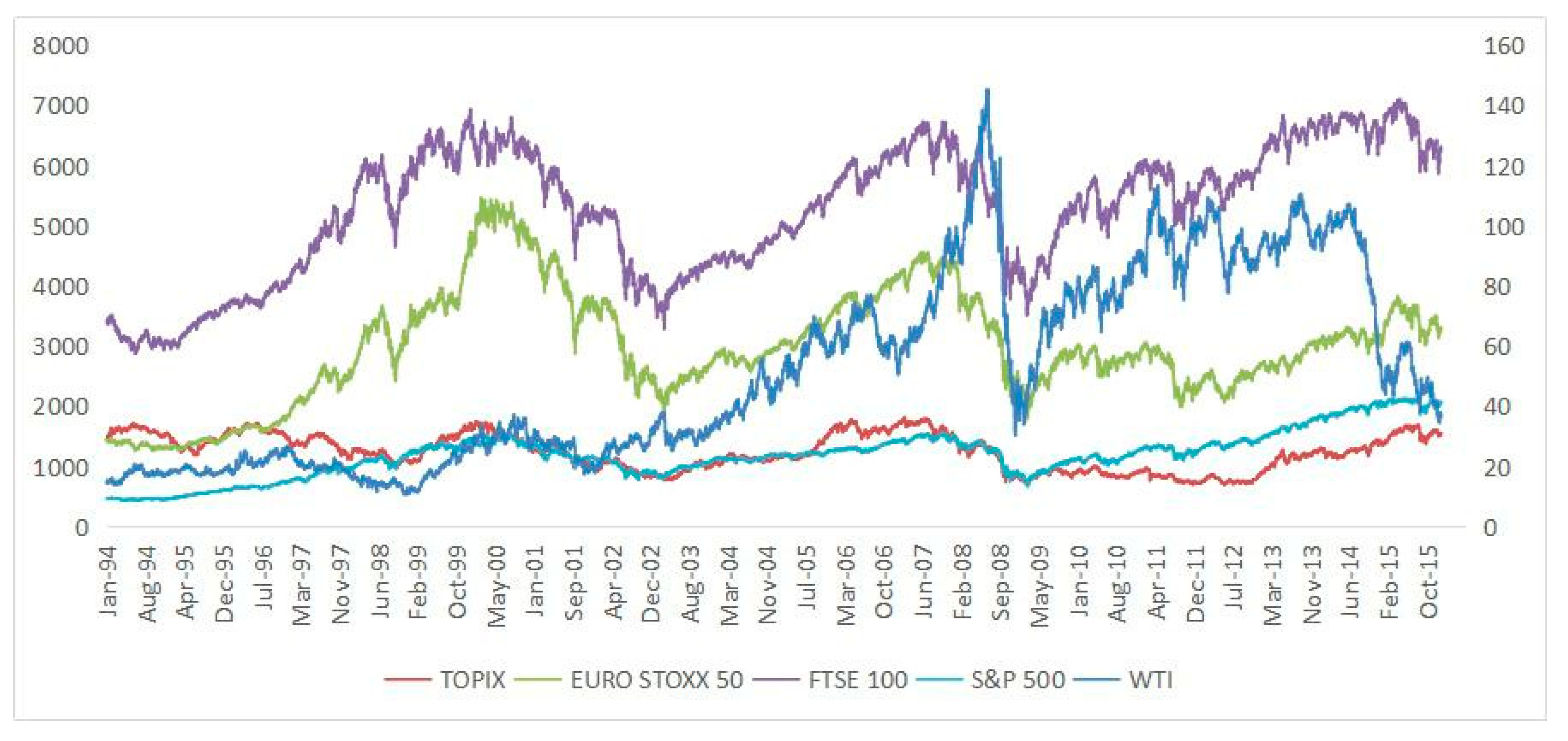
We employed the daily crude oil spot price and daily stock market price indexes to investigate the correlation between stock and crude oil markets. The West Texas Intermediate (WTI) crude oil spot price was employed to denote the crude oil price, which is the immediate delivery price of West Texas intermediate grade oil. Four major stock market price indexes were used: S&P 500, TOPIX, EURO STOXX 50, and FTSE 100—all of which represent 70% of international stock market caps. Specifically, S&P 500 describes the US market, TOPIX describes the Japanese stock market, EURO STOXX 50 describes the European stock market, and FTSE 100 describes the Britain stock market, respectively. All data were obtained from DataStream. The sample spanned from 3 January 1994 to 31 December 2015. We calculated the market returns by the first log difference times 100. The raw data are illustrated in Figure 1.

Table 1. Summary statistics for returns on oil and stock prices. WTI: West Texas Intermediate.

	WTI	TOPIX	EURO 50	FTSE	S&P500
Mean	0.0168	0.0013	0.0144	0.0105	0.0257
Median	0.0000	0.0000	0.0299	0.0063	0.0288
Std. Dev.	0.0237	0.0131	0.0140	0.0114	0.0116
Skewness	−0.1759	−0.269	−0.0531	−0.1632	−0.2469
Kurtosis	7.9511	9.2294	7.6989	9.1743	11.708
Jarque–Bera	5891.576 ***	9349.003 ***	5282.556 ***	9141.575 ***	18,195.04 ***
Obs	5739	5739	5739	5739	5739

Notes: *** indicates significance at the 1% level. Jarque–Bera is a statistical test for normality. Obs is the sample size.

summarizes the descriptive statistics of the returns on the stock and crude oil market. Meanwhile, as suggested by the Jarque–Bera (JB) test, the returns series did not follow the normal distribution in all cases.

2.5. Empirical Results

In this section, we provide the empirical results of the GARCH–MIDAS model in

Table 2. Estimations of generalized autoregressive conditional heteroskedasticity–mixed data sampling (GARCH–MIDAS) coefficients for returns on oil and stock market prices.

	WTI	TOPIX	EURO 50	FTSE	S&P500
$\mu \times {10}^{-5}$	33.82	41.11	64.13	40.02	−52.17
	(27.76)	(15.82) ***	(16.26) ***	(12.07) ***	(12.86) ***
α	0.114	0.099	0.098	0.115	0.098
	(0.009) ***	(0.006) ***	(0.006) ***	(0.009) ***	(0.006) ***
β	0.664	0.869	0.864	0.836	0.867
	(0.031) ***	(0.011) ***	(0.012) ***	(0.014) ***	(0.012) ***
θ	0.203	0.103	0.167	0.180	0.155
	(0.005) ***	(0.028) ***	(0.011) ***	(0.010) ***	(0.011) ***
${\omega }_v$	23.21	4. 648	7.818	9.697	8.50
	(2.469) **	(2.236) **	(2.387) ***	(2.354) ***	(2.507) ***
m × 10−3	9.561	11.81	8.871	6.040	7.594
	(0.750) ***	(0.956) ***	(0.751) ***	(0.553) ***	(0. 614) ***
QL1	11,975.6	14,896.6	14,672.7	15,902.4	15,820.4
AIC	−23,939.2	−29,781.2	−29,333.4	−31,792.8	−31,628.8
BIC	−23,899.3	−29,741.3	−29,293.4	−31,752.9	−31,588.9

Notes: The number of MIDAS lags is 36 for the GARCH processes. The sample size was 5739 and the adjusted sample size was 4983, which covers the period from 26 November 1996 until 31 December 2015. QL₁ represents the log likelihood ratio. The numbers in parentheses are standard errors. *** and ** indicate significance at the 1% and 5% levels, respectively.

. Except for decay parameters, which are significant at the 5% level, all almost parameters are significant at the 1% level. The results indicate that the short-run volatility is the mean reverting to the long-term trend with the justification of the stationary condition. The value of the decay parameter $\omega$ is greater than one which indicates a rapidly decreasing weighting function on the decay pattern. Figure 2 illustrates the dynamics of short- and long-term conditional volatilities, in which we can see that the volatility reached its peak for all markets when the 2008 global financial crisis occurred. In contrast, the 1997 Asian financial crisis showed a lesser influence on these markets.

Additionally, the long-term conditional volatilities are less volatile compared to the short-term conditional volatilities. Nevertheless, it still captures the extreme condition when the short-term conditional volatilities are high. For example, during the 2008 global financial crisis, the short-term conditional volatilities reach their peak while the long-term conditional volatilities exhibit the same properties. Therefore, we confirm our results.

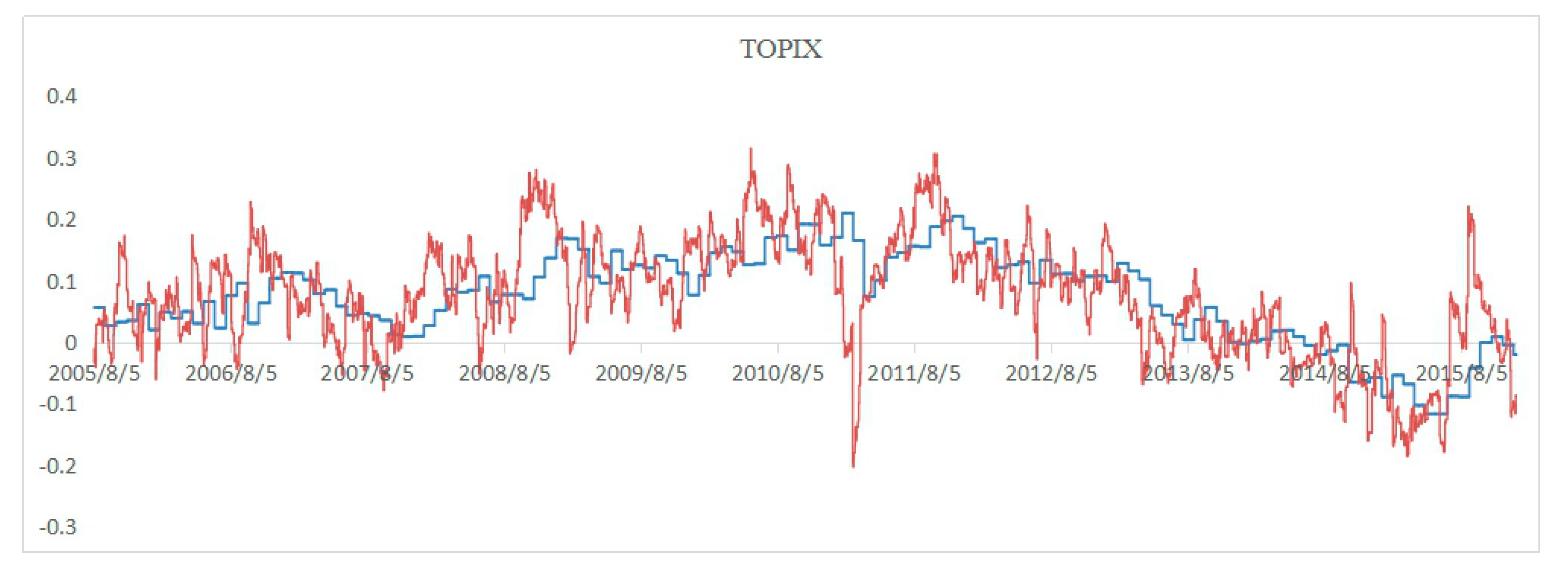
We report the results of the DCC–MIDAS model in

Table 3. Estimations of dynamic conditional correlation (DCC)–MIDAS coefficients between returns on oil and stock market prices.

	TOPIX	EURO 50	FTSE	S&P500
a	0.027	0.032	0.033	0.038
	(0.013) ***	(0.005) ***	(0.007) ***	(0.005) ***
b	0.851	0.946	0.948	0.943
	(0.078) ***	(0.019) ***	(0.018) ***	(0.011) ***
ωr	7.853	26.455	25.131	25.125
	(4.058) **	(12.581) **	(16.932) **	(12.420) **
QL2	−6038.071	−5929.785	−5872.521	−5818.261
AIC	12,082.157	11,865.670	11,751.252	11,642.502
BIC	12,102.129	11,885.582	11,771.111	11,662.541

Notes: The number of MIDAS lags is 144 for the DCC processes. The sample size was 5739, and the adjusted sample size was 2139, which covers the period from 5 August 2005 to 31 December 2015. QL₂ represents the log likelihood ratio. The numbers in parentheses are standard errors. *** and ** indicate significance at the 1% and 5% levels, respectively.

. We set $N_v^i$ as equal to 21 to estimate the monthly DCC between the stock and crude oil markets. Moreover, a Fisher’s Z transformation (to ensure the conditional correlation belongs to normal distribution, we employ Fisher’s Z transformation of ${\rho }_{ij,t}=\ln (\frac{1+{\rho }_{ij,t}}{1-{\rho }_{ij,t}})$) is implemented to identify the long-term conditional correlation between the stock and crude oil markets (Colacito et al. [10]; Beine and Candelon [47]). Similarly, all parameters are significant at the 5% level with the justification of the stationary condition. Note that to generate the pattern of decay, the decay $\omega$ is larger than 1 for all cases, that is, the weight on past-realized return variances decreases rapidly as the DCC–MIDAS model’s lags increase. Figure 3 plots the dynamic correlations between the stock and crude oil markets in both short- and long-term perspectives.

Figure 3 reveals that the dynamic correlations between stock market prices and oil prices are positive, except during the 2008 global financial crisis. To obtain the long-term conditional correlations, the model discards the 3600 observations and thus the adjusted samples period starts from August 2005. Our findings are consistent with the studies by Aloui and Aïssa [41] in that the short-term dynamic correlations are significantly influenced by the global financial crisis. However, the global financial crisis has little effect on their long-term correlation. In Figure 3, we identify a significant decrease in dynamic correlations in the long-term during the 2008 global financial crisis period, indicating that crude oil can provide effective risk diversification during financial turmoil.

3. Identification of Factors

3.1. Data

Next, we attempted to investigate the factors that can influence the dynamic correlation between the stock and crude oil markets in the long term. The monthly data on economic and financial variables from August 2005 to December 2015 were applied for the UK, Japan, the EU, and the US. In order to obtain the long-term conditional correlations, the model discarded the 3600 observations due to the 144 lags of MIDAS. Therefore, the adjusted samples period starts from August 2005. Following Bachmeier et al. [48] and Bachmeier and Cha [49], we used economic activity and inflation as macroeconomic variables. Specifically, we employed the Organization for Economic Co-operation and Development (OECD) composite leading indicator to reflect real economic activities, which indicates a favorable economic outlook when the rate is positive and vice versa. Following Pyun and An [50], Ferrer et al. [51], and Li [52], the terms spread, credit spread, and free rate are classified as financial variables.

Table 4. Summary statistics of variables.

	cc	gr	inf	rf	cr	Ts
Mean	0.205	0.425	1.885	1.130	0.363	1.409
Std. Dev.	0.193	1.808	1.802	1.722	0.397	1.037
Maximum	0.599	4.543	8.70	5.898	3.185	3.757
Minimum	−0.15	−7.058	−2.500	−0.475	−0.017	−0.995
Number of cross-sections	4	4	4	4	4	4
Number of observations	500	500	500	500	500	500

Notes: gr = economic activity, inf = inflation rate, rf = risk-free rate, cr = credit spread, and ts = term spread.

indicates the summary statistics. All data were obtained from DataStream.

3.2. Model and Empirical Results

Following Aloui and Aïssa [41], we constructed a regression model as follows:

$$c{c}_{i,\tau }={\gamma }_0+{\gamma }_{1}g{r}_{i\tau }+{\gamma }_{2}in{f}_{i\tau }+{\gamma }_{3}r{f}_{i\tau }+{\gamma }_{4}c{r}_{i\tau }+{\gamma }_{5}t{s}_{i\tau }+{\mu }_i+{\delta }_t+{\nu }_{i\tau },$$

(14)

where $c{c}_{i,\tau }$ denotes the conditional correlation at time $\tau$, ${\gamma }_0$ denotes constant, $g{r}_{i\tau }$ denotes the growth rate of country $i$ at time $t$, $in{f}_{i\tau }$ denotes the inflation of country $i$ at time $\tau$, $r{f}_{i\tau }$ denotes the risk-free rate of country $i$ at time $\tau$, $c{r}_{i\tau }$ denotes the credit risk of country $i$ at time $\tau$, $t{s}_{i\tau }$ denotes the term spread of country $i$ at time $\tau$, ${\mu }_i$ denotes the time-invariant individual effect of country $i$ at time $\tau$, ${\delta }_t$ denotes the time-specific intercept, and $v_{i\tau }$ denotes the error term of country $i$ at time $\tau$. Specifically, $\tau$ denotes a one-month span in this section.

For economic variables in Equation (14), we selected the annualized inflation rate and annualized composite leading indicator (CLI) to reflect real economic activities. Three financial variables were applied: term spread, credit risk, and risk-free rate.

Table 5. Definition of variables.

Variable	Definition
Panel A: Explained variable
Conditional correlation (cc)	The long-term conditional correlation between oil and stock returns is calculated using the DCC–MIDAS model. Therefore, there are only four groups of long-term conditional correlations; that is, the pairs between oil and TOPIX returns, oil and EURO 50 returns, oil and FTSE returns, and oil and S&P 500 returns. We employ Fisher Z transformation to adjust for the potential problem of non-normality in the conditional correlation.
Panel B: Explanatory variables: macroeconomic variables
Economic activity (gr)	Economic activity is the annualized growth rate (%) of the Organisation for Economic Co-operation and Development (OECD) composite leading indicator in the country.
Inflation (inf)	Inflation is annualized growth rate (%) of Consumer Price Index (CPI) in the country.
Panel C: Explanatory variables: financial variables
Risk-free rate (rf)	Risk-free rate refers to the three-month government bill yield in the country.
Credit risk (cr)	Credit risk is calculated as the difference between the three-month interbank rate and three-month government bill yield in the country. The variable measures the credit risk of the banking system.
Term spread (ts)	Term spread is defined as the difference between the long-term 10-year government bond yield and the three-month government bill yield in the country.

summarizes the definitions of these variables.

As a benchmark, the results of the pooled ordinary least squares method (Model 1) are reported in

Table 6. Estimation results for panel data analysis.

	Model 1	Model 2	Model 3	Model 4	Model 5
${\gamma }_0$	0.069	0.181	0.297	0.223	0.283
	(0.082)	(0.069) ***	(0.086) ***	(0.024) ***	(0.023) ***
gr	−0.005	−0.004	−0.019	−0.029
	(0.001) ***	(0.001) ***	(0.005) ***	(0.011) ***
$inf$	0.037	0.027	0.007	−0.002
	(0.012) ***	(0.015) *	(0.007)	(0.011)
rf	−0.012	−0.043	0.046	-	−0.042
	(0.022)	(0.012) **	(0.019) **		(0.008) ***
cr	−0.130	−0.131	−0.133	-	−0.132
	(0.065) **	(0.068)	(0.063) ***		(0.054) **
ts	0.091	0.044	0.003	-	0.012
	(0.034) ***	(0.025) *	(0.028)		(0.027)
R2	0.465	0.547	0.665	0.475	0.630
Adjusted R2	0.460	0.540	0.661	0.470	0.625
LL	270.082	311.755	326.121	270.549	316.204
H test	68.227 ***

Notes: Model 1 was estimated using the pooled ordinary least squares method. Model 2 was estimated using a fixed effects model. Models 3, 4, and 5 were estimated using fixed effects models with time dummies. The numbers in parentheses are White robust standard errors. LL represents the log likelihood ratio. H test indicates the Hausman test. ***, ** and * indicate significance at the 1%, 5% and 10% levels, respectively. R² denotes the within coefficient of determination.

. Regarding panel analysis, we consider the fixed effects of our panel regression as suggested by the Hausman test. In addition, because there were only four groups in our dataset, which are much smaller than the time period (100 months), we incorporated the time effects into the fixed effects model in order to consider the possible structural changes (Models 3, 4, and 5). We found that only risk-free rate has a positive influence on the dynamic correlation, whereas both credit risk and economic activity have a negative effect on the dynamic correlation between stock and crude oil returns. Moreover, Models 4 and 5 provide additional evidence to support the estimation of Model 3. However, the results from Model 4 do not seem to support inflation rate as a factor.

3.3. Robustness Check

Since the length of the time series is much larger than the number of cross sections, our sample behaves more like time-series data than panel data. Therefore, to increase the robustness of our empirical results, the one-period-lagged term of the independent variable is used as an explanatory variable. Thus, we obtain

$${\mathrm{cc}}_{i,\tau }={\gamma }_0+{\gamma }_{1}g{r}_{i\tau -1}+{\gamma }_{2}in{f}_{i\tau -1}+{\gamma }_{3}r{f}_{i\tau -1}+{\gamma }_{4}c{r}_{i\tau -1}+{\gamma }_{5}t{s}_{i\tau -1}+{\mu }_i+{\delta }_t+{\nu }_{i\tau }$$

(15)

Similarly to Equation (14), Equation (15) incorporated the fixed effects into the panel regression model as suggested by the Hausman test. According to

Table 7. Estimation results for panel data analysis.

	Model 6	Model 7	Model 8	Model 9	Model 10
${\gamma }_0$	0.064	0.183	0.304	0.223	0.283
	(0.017) ***	(0.073) **	(0.021) ***	(0.008) ***	(0.023) ***
gr(−1)	−0.006	−0.005	−0.019	−0.028	-
	(0.006)	(0.008)	(0.005) ***	(0.011) ***
$inf\left(-1\right)$	0.034	0.023	0.006	−0.003	-
	(0.011) ***	(0.014)	(0.007)	(0.011)
fr(−1)	0.010	−0.043	0.048	-	−0.044
	(0.021)	(0.012) ***	(0.021) ***		(0.017) **
cr(−1)	−0.108	−0.088	−0.122	-	−0.122
	(0.067)	(0.071)	(0.055) **		(0.045)**
ts(−1)	0.094	0.044	0.004	-	0.010
	(0.034) ***	(0.026) *	(0.031)		(0.031)
R2	0.480	0.537	0.667	0.480	0.631
Adjusted R2	0.444	0.530	0.662	0.474	0.626
LL	261.571	304.699	323.225	304.111	312.154
H test	74.675 ***

Notes: Model 6 was estimated using the pooled ordinary least squares method. Model 7 was estimated using a fixed effects model. Models 8, 9, and 10 were estimated using fixed effects models with time effects. The numbers in parentheses are White robust standard errors. LL represents the log likelihood ratio. H test indicates the Hausman test. ***, ** and * indicate significance at the 1%, 5% and 10% levels, respectively. R² denotes the within coefficient of determination.

, the empirical results in Model 8 confirm that risk-free rate and economic activity are important factors in determining the dynamic correlation between stock and crude oil markets. Specifically, risk-free rate has a positive effect on conditional correlation, while economic activity has a negative effect. Similarly to the results of Equation (14), financial factors are still significant. Moreover, Models 9 and 10 also confirm that economic activity and credit risk are important factors in determining the dynamic correlation between stock and crude oil markets.

The interpretation of these results is relatively straightforward. According to Bachmeier and Cha [49], a rise of the risk free rate increases the nominal returns on both the stock and crude oil markets. In addition, the relative strength of an economy raises stock market prices, with a relative decrease in oil price returns, as the currency of this economy appreciates (Basher et al. [53]). Note that the conditional correlation between the stock and crude oil markets is negatively influenced by credit risk, implying that the oil market serves as an alternative asset during periods of economic downturn. In summary, during times of economic recession, the stock market declines as the oil market rises. Moreover, we found that both the adjusted within-R² and log likelihood are larger for the financial sector than for the macroeconomic sector, indicating that the financial sector will provide more explanation of the co-movement between the stock and crude oil markets.

4. Conclusions

This article investigated the financial and macroeconomic factors that influence the monthly correlation between crude stock and crude oil markets by employing the MIDAS approach and panel data analysis.

In the analysis of the monthly volatility in the stock and crude oil markets, we identified the 2008 global financial crisis as significantly increasing volatility for all markets. By contrast, the 1997 Asian financial crisis had a lower impact on these markets. Furthermore, by employing the DCC–MIDAS model, we investigated the conditional correlation between the stock and crude oil markets in the long term and obtained the following findings. First, the long-term conditional correlations between stock and crude oil markets are positive for all cases, except during 2008 global crisis periods. Second, the Japanese stock market prices show the smallest degree of correlation with oil prices, while the UK stock market prices show the largest degree of correlation. Third, the 2008 global financial crisis had little impact on the long-term correlation between stock and crude oil markets.

We ran panel regressions to further explore the factors that can affect the long-term conditional correlation between the stock and crude oil markets. The results of our panel regression analysis reveal that both economic activity and credit risk have a negative effect on the correlation between stock and crude oil markets in the long-term. However, the long-term correlation between crude oil and stock markets increases with increases in the risk-free rate. Our empirical results imply that a rise in the risk-free rate increases the conditional correlation between crude oil and stock returns in the long-term, while an increase in economic activity or credit risk decreases the conditional correlation in the long-term.

The reasons for these conclusions are twofold. From an economic perspective, a rise in risk-free rate in one country increases the nominal returns on both the stock and crude oil markets. Moreover, relative strength in the economy raises stock market prices, with a relative decrease in the returns on oil prices, since the currency in such an economy appreciates. From a financial perspective, stock prices decline owing to a relatively high risk-free rate environment in one country, whereas the crude oil prices remain independent in such an environment. Moreover, crude oil futures or crude oil-related derivatives may serve as a good hedge asset when the credit risk increases as the stock market slumps.

At least two policy implications can be provided by our research. From an economic perspective, because risk-free rate has a positive impact on the correlation between the stock and crude oil markets, we notice that the inflationary environment works effectively in asset pricing. Therefore, monetary authorities must be prudent when implementing their monetary policies. From a financial perspective, a diversification benefit exists between stocks and crude oil, especially during periods of financial crisis.

References

- Hamilton, J.D. Oil and the Macroeconomy since World War II. J. Polit. Econ. 1983, 91, 228–248. [Google Scholar] [CrossRef]
- Kanjilal, K.; Ghosh, S. Co-movement of international crude oil price and Indian stock market: Evidences from nonlinear cointegration tests. Energy Econ. 2016, 53, 111–117. [Google Scholar]
- Filis, G.; Degiannakis, S.; Floros, C. Dynamic correlation between stock market and oil prices: The case of oil-importing and oil-exporting countries. Int. Rev. Financ. Anal. 2011, 20, 152–164. [Google Scholar] [CrossRef]
- Arouri, M.E.H.; Jouini, J.; Nguyen, D.K. On the impacts of oil price fluctuations on European equity markets: Volatility spillover and hedging effectiveness. Energy Econ. 2012, 34, 611–617. [Google Scholar] [CrossRef]
- Tamakoshi, G.; Hamori, S. An asymmetric dynamic conditional correlation analysis of linkages of European financial institutions during the Greek sovereign debt crisis. Eur. J. Financ. 2013, 19, 939–950. [Google Scholar] [CrossRef]
- Tamakoshi, G.; Hamori, S. Co-movements among major European exchange rates: A multivariate time-varying asymmetric approach. Int. Rev. Econ. Financ. 2014, 31, 105–113. [Google Scholar] [CrossRef]
- Basher, S.A.; Sadorsky, P. Hedging emerging market stock prices with oil, gold, VIX, and bonds: A comparison between DCC, ADCC and GO-GARCH. Energy Econ. 2016, 54, 235–247. [Google Scholar] [CrossRef] [Green Version]
- Büyükşahin, B.; Robe, M.A. Speculators, commodities and cross-market linkages. J. Int. Money Financ. 2014, 42, 38–70. [Google Scholar]
- Silvennoinen, A.; Thorp, S. Financialization, crisis and commodity correlation dynamics. J. Int. Financ. Mark. Inst. Money 2013, 24, 42–65. [Google Scholar] [CrossRef] [Green Version]
- Colacito, R.; Engle, R.F.; Ghysels, E. A component model for dynamic correlations. J. Econ. 2011, 164, 45–59. [Google Scholar] [CrossRef] [Green Version]
- Aloui, C.; Jammazi, R. The effects of crude oil shocks on stock market shifts behaviour: A regime switching approach. Energy Econ. 2009, 31, 789–799. [Google Scholar] [CrossRef]
- Chen, S.-S. Do higher oil prices push the stock market into bear territory? Energy Econ. 2010, 32, 490–495. [Google Scholar] [CrossRef]
- Ghouri, S.S. Assessment of the relationship between oil prices and US oil stocks. Energy Policy 2006, 34, 3327–3333. [Google Scholar] [CrossRef]
- Jones, C.M.; Kaul, G. Oil and the stock markets. J. Financ. 1996, 51, 463–491. [Google Scholar] [CrossRef]
- Kilian, L. Not All Oil Price Shocks Are Alike: Disentangling Demand and Supply Shocks in the Crude Oil Market. Am. Econ. Rev. 2009, 99, 1053–1069. [Google Scholar] [CrossRef]
- Miller, J.I.; Ratti, R.A. Crude oil and stock markets: Stability, instability, and bubbles. Energy Econ. 2009, 31, 559–568. [Google Scholar] [CrossRef] [Green Version]
- Sadorsky, P. Oil price shocks and stock market activity. Energy Econ. 1999, 21, 449–469. [Google Scholar] [CrossRef]
- Papapetrou, E. Oil price shocks, stock market, economic activity and employment in Greece. Energy Econ. 2001, 23, 511–532. [Google Scholar] [CrossRef]
- Chen, N.-F.; Roll, R.; Ross, S.A. Economic Forces and the Stock Market. J. Bus. 1986, 59, 383–403. [Google Scholar] [CrossRef]
- El-Sharif, I.; Brown, D.; Burton, B.; Nixon, B.; Russell, A. Evidence on the nature and extent of the relationship between oil prices and equity values in the UK. Energy Econ. 2005, 27, 819–830. [Google Scholar] [CrossRef]
- Narayan, P.K.; Narayan, S. Modelling the impact of oil prices on Vietnam’s stock prices. Appl. Energy 2010, 87, 356–361. [Google Scholar] [CrossRef]
- Li, S.-F.; Zhu, H.-M.; Yu, K. Oil prices and stock market in China: A sector analysis using panel cointegration with multiple breaks. Energy Econ. 2012, 34, 1951–1958. [Google Scholar] [CrossRef]
- Zhu, H.-M.; Li, R.; Li, S. Modelling dynamic dependence between crude oil prices and Asia-Pacific stock market returns. Int. Rev. Econ. Financ. 2014, 29, 208–223. [Google Scholar] [CrossRef]
- Narayan, P.K.; Gupta, R. Has oil price predicted stock returns for over a century? Energy Econ. 2015, 48, 18–23. [Google Scholar] [CrossRef] [Green Version]
- Jiménez-Rodríguez, R. Oil price shocks and stock markets: Testing for non-linearity. Empir. Econ. 2015, 48, 1079–1102. [Google Scholar]
- Ponka, H. Real oil prices and the international sign predictability of stock returns. Fin. Res. Lett. 2017, 17, 79–87. [Google Scholar] [CrossRef]
- Arouri, M.E.H.; Jouini, J.; Nguyen, D.K. Volatility spillovers between oil prices and stock sector returns: Implications for portfolio management. J. Int. Money Financ. 2011, 30, 1387–1405. [Google Scholar] [CrossRef]
- Arouri, M.E.H.; Lahiani, A.; Nguyen, D.K. Return and volatility transmission between world oil prices and stock markets of the GCC countries. Econ. Model. 2011, 28, 1815–1825. [Google Scholar] [CrossRef] [Green Version]
- Conrad, C.; Loch, K.; Rittler, D. On the macroeconomic determinants of long-term volatilities and correlations in U.S. stock and crude oil markets. J. Empir. Financ. 2014, 29, 26–40. [Google Scholar] [CrossRef]
- Malik, F.; Ewing, B.T. Volatility transmission between oil prices and equity sector returns. Int. Rev. Financ. Anal. 2009, 18, 95–100. [Google Scholar] [CrossRef]
- Malik, F.; Hammoudeh, S. Shock and volatility transmission in the oil, US and Gulf equity markets. Int. Rev. Econ. Financ. 2007, 16, 357–368. [Google Scholar] [CrossRef]
- Sadorsky, P. Correlations and volatility spillovers between oil prices and the stock prices of clean energy and technology companies. Energy Econ. 2012, 34, 248–255. [Google Scholar] [CrossRef]
- Sadorsky, P. Modeling volatility and correlations between emerging market stock prices and the prices of copper, oil and wheat. Energy Econ. 2014, 43, 72–81. [Google Scholar] [CrossRef]
- Bampinas, G.; Panagiotidis, T. Oil and stock markets before and after financial crises: A local Gaussian correlation approach. J. Future Mark. 2017, 37, 1179–1204. [Google Scholar] [CrossRef]
- Yin, L. Does oil price respond to macroeconomic uncertainty? New evidence. Empir. Econ. 2016, 51, 921–938. [Google Scholar] [CrossRef]
- Nguyen, D.K. Walther, T. Modelling and forecasting commodity market volatility with long-term economic and financial variables. J. Forecast 2019, 1, 1–17. [Google Scholar]
- Kilian, L. Measuring global real economic activity: Do recent critiques hold up to scrutiny? Econ. Lett. 2019, 178, 106–110. [Google Scholar] [CrossRef] [Green Version]
- Kilian, L.; Park, C. The impact of oil price shocks on the U.S. Stock market. Int. Econ. Rev. 2009, 50, 1267–1287. [Google Scholar] [CrossRef]
- Aloui, R.; Hammoudeh, S.; Nguyen, D.K. A time-varying copula approach to oil and stock market dependence: The case of transition economies. Energy Econ. 2013, 39, 208–221. [Google Scholar] [CrossRef]
- Martín-Barragán, B.; Ramos, S.B.; Veiga, H. Correlations between oil and stock markets: A wavelet-based approach. Econ. Modell. 2015, 50, 212–227. [Google Scholar] [CrossRef]
- Aloui, R.; Ben Aïssa, M.S. Relationship between oil, stock prices and exchange rates: A vine copula based GARCH method. N. Am. J. Econ. Financ. 2016, 37, 458–471. [Google Scholar] [CrossRef]
- Cai, X.J.; Tian, S.; Yuan, N.; Hamori, S. Interdependence between oil and East Asian stock markets: Evidence from wavelet coherence analysis. J. Int. Financ. Mark. Inst. Money 2017, 48, 206–223. [Google Scholar] [CrossRef]
- Engle, R. Dynamic conditional correlation: A simple class of multivariate GARCH models. J. Bus. Econ. Stat. 2002, 20, 339–350. [Google Scholar] [CrossRef]
- Yang, L.; Cai, X.J.; Hamori, S. What determines the long-term correlation between oil prices and exchange rates? N. Am. J. Econ. Financ. 2018, 44, 140–152. [Google Scholar] [CrossRef]
- Engle, R.F.; Ghysels, E.; Sohn, B. On the Economic Sources of Stock Market Volatility. Rev. Econ. Stud. 2013, 95, 779–797. [Google Scholar] [CrossRef]
- Engle, R.; Rangel, J.G. The spline GARCH model for unconditional volatility and its global macroeconomic sources. Rev. Financ. Stud. 2008, 21, 1187–1222. [Google Scholar] [CrossRef]
- Beine, M.; Candelon, B. Liberalization and stock market co-movement between emerging economies. Quant. Financ. 2011, 11, 299–312. [Google Scholar] [CrossRef]
- Bachmeier, L.; Li, Q.; Liu, D. Should oil prices receive so much attention? an evaluation of the predictive power of oil prices for the U.S. economy. Econ. Inq. 2008, 46, 528–539. [Google Scholar] [CrossRef]
- Bachmeier, L.J.; Cha, I. Why Don’t Oil Shocks Cause Inflation? Evidence from Disaggregate Inflation Data. J. Money Credit Bank. 2011, 43, 1165–1183. [Google Scholar] [CrossRef]
- Pyun, J.H.; An, J. Capital and credit market integration and real economic contagion during the global financial crisis. J. Int. Money Financ. 2016, 67, 172–193. [Google Scholar] [CrossRef]
- Ferrer, R.; Bolós, V.J.; Benítez, R. Interest rate changes and stock returns: A European multi-country study with wavelets. Int. Rev. Econ. Financ. 2016, 44, 1–12. [Google Scholar] [CrossRef]
- Li, M.C. US term structure and international stock market volatility: The role of the expectations factor and the maturity premium. J. Int. Financ. Mark. Inst. Money 2016, 41, 1–15. [Google Scholar] [CrossRef]
- Basher, S.A.; Haug, A.A.; Sadorsky, P. Oil prices, exchange rates, and emerging stock market prices. Energy Econ. 2012, 34, 227–240. [Google Scholar] [CrossRef]
Figure 1.
Plots of raw data. The left axis denotes the stock market price index, while the right axis denotes the crude oil price.
Figure 2.
Short- and long-term volatilities for crude oil (WTI, TOPIX, EURO STOXX 50, FTSE 100, and S&P 500). The red line indicates the short-term volatility, while the blue line indicates the long-term volatility.
Figure 3.
Short- and long-term DCC–MIDAS correlations between oil and stock market prices at the aggregated levels for four country groups; that is, TOPIX, EURO STOXX 50, FTSE 100, and S&P 500. The red line indicates the short-term DCC, while the blue line indicates the long-term DCC–MIDAS correlation.