Developing a Data Mining Based Model to Extract Predictor Factors in Energy Systems: Application of Global Natural Gas Demand

Abstract

Recently, the natural gas (NG) global market attracted much attention as it is cleaner than oil and, simultaneously in most regions, is cheaper than renewable energy sources. However, price fluctuations, environmental concerns, technological development, emerging unconventional resources, energy security challenges, and shipment are some of the forces made the NG market more dynamic and complex. From a policy-making perspective, it is vital to uncover demand-side future trends. This paper proposed an intelligent forecasting model to forecast NG global demand, however investigating a multi-dimensional purified input vector. The model starts with a data mining (DM) step to purify input features, identify the best time lags, and pre-processing selected input vector. Then a hybrid artificial neural network (ANN) which is equipped with genetic optimizer is applied to set up ANN’s characteristics. Among 13 available input features, six features (e.g., Alternative and Nuclear Energy, CO₂ Emissions, GDP per Capita, Urban Population, Natural Gas Production, Oil Consumption) were selected as the most relevant feature via the DM step. Then, the hybrid learning prediction model is designed to extrapolate the consumption of future trends. The proposed model overcomes competitive models refer to different five error based evaluation statistics consist of R², MAE, MAPE, MBE, and RMSE. In addition, as the model proposed the best input feature set, results compared to the model which used the raw input set, with no DM purification process. The comparison showed that DmGNn overcame dramatically a simple GNn. Also, a looser prediction model, such as a generalized neural network with purified input features obtained a larger R² indicator (=0.9864) than the GNn (=0.9679).

1. Introduction

The world energy demand increased in the two past decades and even predictions implying the growing trends for the next decades [1,2,3,4]. Still, fossil fuels play a critical role in the energy supply chain due to economic feasibility. Refer to International Energy Agency’s (IEA) 2016 report, fossil fuels in the form of liquid fuels, natural gas, and coal contain more than 80% of the world energy consumption [5]. Easiness of utilization, higher performance, compared to traditional energy sources, ease of mobility via land or sea, and affordable extraction cost introduced oil and natural gas (NG) as strategic commodities [6,7,8]. However, emergent ecological concerns and rethinking of a more peaceful future (sustainable development goals) attracted attention toward climate change challenges (such as greenhouse gases emissions and global warming) [9]. The two non-aligned objectives, on one hand, development and increasing needs for energy supply and on the other hand global environmental concerns, attracted researchers to study energy systems and develop different plausible future perspectives.

World’s economic growth still strongly correlated with the energy and, as a result, the energy price influence potential future trends. The 1970’s energy crisis represented how energy shocks can cause chaotic behavior of economic systems especially in the case of developed countries which mostly play in energy markets as importers. Although new paradigms emerged to address the modern world energy challenges, such as evaluating and improving the energy security level, but policymakers are facing deep uncertainties in this area. Energy markets are known as complex systems [10,11], which consist of numerous players with conflict of interests and changing rules.

Despite successful efforts, the main problem is still existing, which is defined as “discovering reliable future trends and probable alternative futures in the field of energy systems and uncover the most influencing driving forces to aid energy management process”. To project a reliable future, it is crucial to investigating almost all informative input features which represent historical behavior of the targeted complex system and extrapolate future trends. Studying different input features means to peruse different aspects, while on the other hand, it means more efforts in term of cost, time, and complicated estimator. A traditional approach to address a complex problem is to simplify and decompose it to its main constituent elements. Feature selection methods are aimed to adjust the unnecessary complexity revealed to refer to the existence of multiple input features. A feature selection method determines the best subset of the initial features set as a representative of the solution space (for more information about feature selection approaches and methods see: [12,13,14,15]). Selected features interpreted as key driving forces which will help to extrapolate future trends. Moreover, pre-processing might also be performed in order to speed up computation [16]. Finally, an estimator is needed to predict future behaviors of the targeted variable. Despite there are many classical methods but artificial intelligence-based methods are extensively used during the last couple of decades [17,18] that attempt to uncover weak signals and pattern more reliable and accurate. As Kourou et al. noted these methods can discover and identify patterns and relationships between them, from complex datasets, while they are able to effectively predict future outcomes [19]. Technologies as Data Mining, Natural Language Processing, and Machine Learning can provide novel alternatives to explore and exploit potential retrieved knowledge from historical records [20], and help to decrease prediction errors effectively.

This paper is aimed to develop an intelligent learning-based prediction model which is equipped with data mining (DM) techniques to purify and the setup input vector. The DM step is used to select and organize the best input features that represent patterns of future global NG demand trends. Although many previous studies successfully addressed NG global demand prediction problem, we attempt to uncover the most effective driving forces as input features and analyzing how they will affect the objective function (NG global demand prediction). For example, the proposed model studies time relation between input variables and the target variable. So a less-dimension input set is available to policymakers to simplify and experience reliable decision-making process.

As it is impressed by a series of variables and oscillating time series, the NG forecasting problem is a very challenging [21]. These days, massive efforts have been investigated artificial intelligence (AI) models or integration of several models (hybrid models) for prediction problems to increase the accuracy and the model reliability [22,23].

2. Literature Review

Also, numerous notable studies have investigated demand prediction for the case of energy resources [24,25,26,27,28,29]. Among those, Baumeister and Kilian published a research paper to analyze how vector autoregression (VAR) models form policy-relevant forecasting scenarios in the case of an oil market. The model investigates the influence of scenario weights’ probability changes to the real-time oil price forecasting [30]. In addition, Dilaver et al. investigated NG consumption in Europe to support long-term investments and contracts [31]. They estimated an OECD-Europe NG demand trends with annual time series during the period from 1978 to 2011 by applying a structural time series model (STSM). Finally, three scenario streams developed based on business as usual, high, and low case scenarios.

Li et al. used system dynamic models to create possible outlooks to 2030 for the case of China’s NG consumption growth. Then to assess the results accuracy and propose policy recommendations on NG exploration and development of China’s NG industry, a scenario analysis step was applied [32]. Also, Suganthi and Samuel provided a comprehensive review of an energy model, which attempted to forecast demand function [33]. Authors classified prediction models and presented that most of the recent researches contained basically quantitative models that result in a single future prediction. Models used statistical error functions to estimate, accuracy compared with other comparative models. However, as mentioned above data-driven models may regret set of effective qualitative variables. In the other hand projecting alternative futures based on qualitative approaches are challenging, especially in the case of validation and, moreover, they are extremely affected by the expert group (number of experts and judgment validation).

Baumeister and Kilian [30] described how vector autoregression (VAR) models can generate policy-relevant forecast scenarios of the global oil market and how real-time oil price forecasting, influenced by possible changes in probability weights, corresponded to the scenarios. In addition, Dilaver et al. [31] investigated natural gas consumption in Europe to support long-term investments and contracts. They implemented a structural time series model (STSM) to estimate the OECD-Europe natural gas demand function with annual data from 1978 to 2011. Using that information, they developed three scenarios based on high-case, reference (business as usual), and low-case scenarios.

Suganthi and Samuel [33] provided a comprehensive review of energy models aimed at forecasting demand functions. The study classified prediction models and identified that most of the recent studies were comprised of quantitative models that provided only a single future prediction scenario. The models predominantly used statistical error functions to estimate accuracy compared with other models. To present a more universal review and to dedicate insights about prediction approaches used by previous studies,

Table 1. Analyzing previous studies, based on their approaches to address energy consumption prediction problem.

Approaches		References
Classical computational extrapolation	Time series	[24,25,31,34,35,36,37,38,39,40,41,42,43]
	Regression	[28,44,45,46,47]
Econometrics		[48,49,50,51,52]
Expert systems and learning models	Artificial neural network (ANN)	[21,40,53,54,55,56,57,58,59,60,61,62,63,64,65,66,67,68,69]
	Genetic programming (GP)	[21,24,40,58,65,67,69,70,71,72,73,74,75,76]
	Ant colony optimization	[77]
	Particle swarm optimization (PSO)	[26,78,79]
	Support vector machine (SVM)	[25,40,59,64,80,81]
	Fuzzy inference system (FIS)	[21,44,62,73,82]
Others	Decomposition approach	[83,84]
	Input-output model	[85,86]
	Bottom-up model	[87,88,89]
	Grey method	[26,37,76,86,90,91]
	Logistic model	[92]

summarized models used to address energy consumption prediction problem.

As shown in Table 1 and noted before learning based techniques can lead to develop a more reliable, accurate estimator as they can represent a self-adjustment characteristic since they learn formerly signals via feedback loops. To dedicate a more detailed understanding of various existed forecasting models,

Table 2. The major pros and cons of main forecasting methods.

Type of Models	Pros & Cons
Classic price modeling/forecasting	Focus on historical data. Do not consider jumps and drips of the prices. Generally, these models were introduced for stock markets. Do not use unit root test for time series and econometric methods to estimate their parameters.
Time series models	Focus on historical data. Do not cope with extreme jumps and drips. Do not use feedback loops to dynamically upgrade model adjustment features.
Learning forecasting models	Focus on historical data. Generally being able to learn fluctuations and related formerly signals. Use feedback loops to upgrade model adjustment features dynamically.
Qualitative based forecasting models	Rarely depend on quantitative forecasting methods. Donate insights about long-run behaviors of a complex system. Mostly depend on experts’ evaluations, instead of historical time series. Are able to dynamically modify input features.

shows the pros and cons of main forecasting methods.

In this paper, we are aimed to propose a learning-based model, which is designed to present a more reliable and relevant input features (driving forces) to initialize a hybrid prediction ANN [93] to equip decision-making process with accurate and reliable forecasts. Next section investigates the proposed methodology and brief descriptions of various steps, then section three is dedicated to presenting the implementation phase and discussing results to show how the proposed methodology overcomes other benchmark models. Finally, section four provides summaries and conclusions.

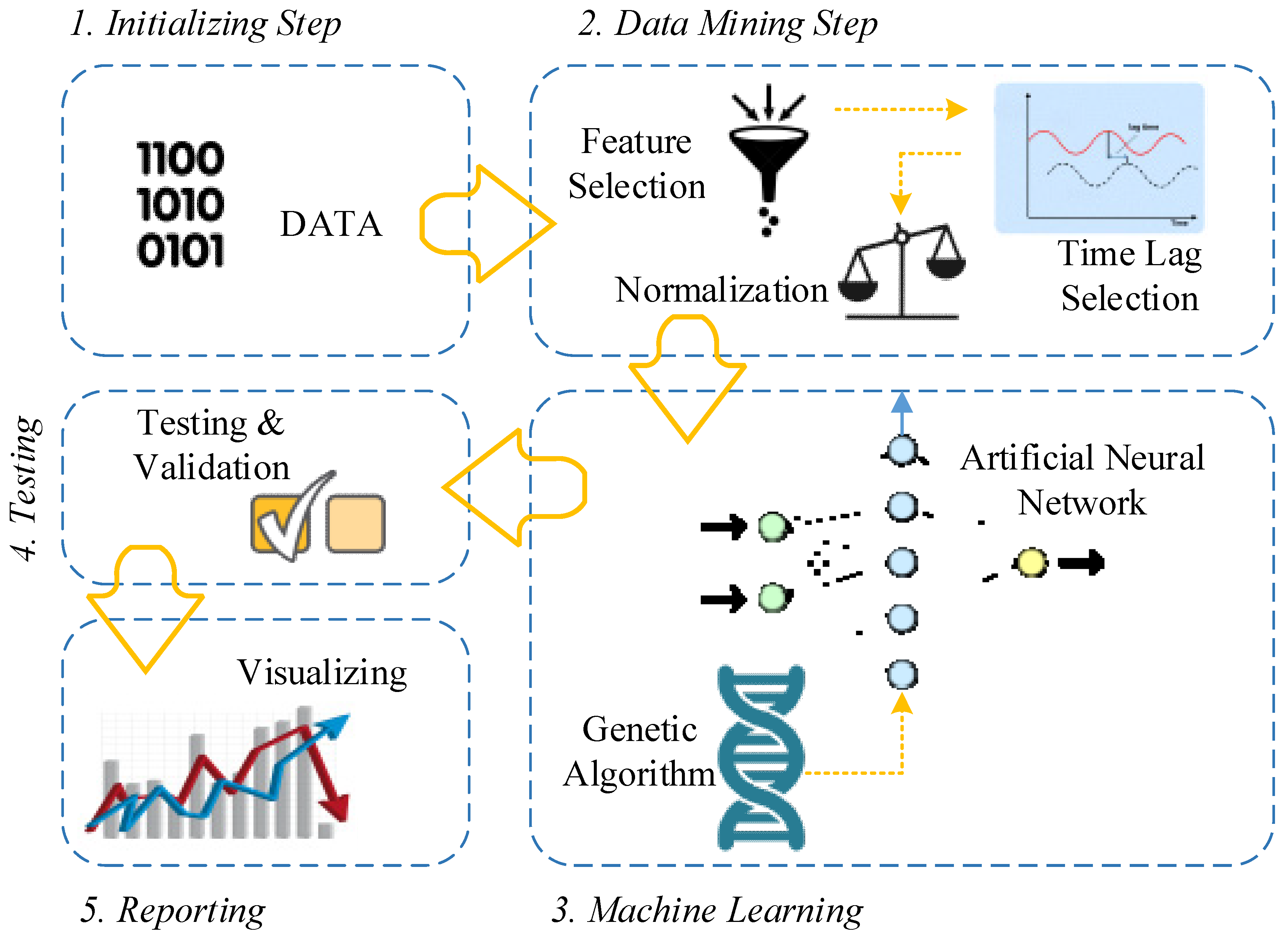
3. The Methodology of Research

As noted previously, the following research is aimed to expand a data mining based prediction model. Three major goals are targeted: (1) determining features which effectively present trends for NG global demand (i.e., driving forces which can shape and define future trends), (2) identification of time lags to define time relations between input variables and the target variable (as inter-correlated features represents their influences with different time lags/delays), and (3) developing a learning intelligent prediction model that can extrapolate future trends for the global NG demands. Figure 1 conceptually shows designed data mining genetic-neural network (DmGNn) methodology to approach noted goals.

Following, the main phases and steps of the proposed methodology are discussed and corresponding outputs are mentioned:

PHASE 1.

Step 1. Data gathering: in this step previous studies reviewed to detect potential input features. Unlike most of the published researches, this paper pursues the maximum approach, means gathering and using maximum available features to ensure that no useful information will be neglected by the estimator. In simple words, the proposed methodology doesn’t immure the solution space due to the use of purified input vector. Output: input feature subset.

PHASE 2.

Step 2. Feature selection: this step is designed to select the most relevant subset of the extracted features. The main objective is to reduce problem dimensions while preserving all local and global optimal solutions (i.e., reliability of the results). Here, the correlation-based feature selection (CFS) [94,95] technique is used to define final input feature subset. Output: refined input feature sub-set.

Step 3. Time lag selection: it is investigated to study how different time lags for input features may affect forecasting accuracy. The theory behind it is that in a complex system elements are inter-correlated but with varying degrees, and sometimes react with different time lags [17]. This step will study time relation between input features and the target variable (natural gas demand). Information criteria [96] method is used to detect lag orders. Output: timed input features subset.

Step 4. Normalization: different scales of input features may cause in a biased final forecasting model [97]. This step is aimed at reproducing input features but in similar, uniform scales. Min-max method [98,99] is used to normalize the input features subset. Output: uniformed timed input features sub-set.

PHASE 3.

Step 5. Design of the forecasting model: in this step, an ANN [100] is equipped with a GA [101] in order to optimize the network’s characteristics and develop an accurate prediction model. Output: estimator.

PHASE 4.

Step 6. Implementation: finalized input features subset are applied to the developed estimator. In this step, the input set is divided into two main portions, one to train (about 80%) and other to test (about 20%) the performance of the prediction framework. Outputs: adjusted prediction model & resulted in extrapolated results.

PHASE 5.

Step 7. Validation: this step is dedicated to comparing the obtained results of the proposed prediction framework with other benchmark comparative models based on multiple error indicators. R², MAE, MAPE, MBE, and RMSE are used to compare prediction results and perform accuracy analysis. Output: accuracy analysis.

To model complex systems (like energy systems), selecting a robust model architecture is very challenging [17,102]. Data mining (DM) techniques are selected to handle the complexity of input variables. DM is defined as the process of extracting appealing patterns and deriving knowledge in massive datasets. Refer to Han et al.: "the principal dimensions are data, knowledge, applications, and technologies" [103]. Following sections are dedicated to present implementation process and obtained results in details.

3.1. Input Preparation

3.1.1. Data Gathering

Input data extremely affect the accuracy and quality of the obtained results. In the case of energy consumption, previous researches investigated different sets of input features to predict energy consumption’s upcoming trends. A significant limitation of a prediction model is that it cannot reflect the effects of variables, which did not exist in the input feature set (those have been neglected). To ensure robustness and the validity of the proposed prediction model, the paper proposes the maximal approach, which means to investigate all available input data and reduce dataset dimension through a DM technique. This approach has the advantage of retaining all signals and trends, while simultaneously the model faces an undeniable challenge that is the increased complexity level due to the large input set, which may negatively affect prediction efficiency. In another hand, it is a challenging process to set up strategic decisions based on a large collection of parameters/inputs. To handle the noted problem, a DM based data pre-processing step is proposed by this paper to examine and purify input features.

Table 3. Initialize input features.

Title	Unit	Reference(s)	Source
Alternative and Nuclear Energy	% of total energy use	Proposed by authors	World Bank
CO2 Emissions	metric tons per capita	[49]	World Bank
CO2 Emissions	Kt		World Bank
Energy Imports, Net	% of energy use	Proposed by authors	World Bank
Fossil Fuel Energy Consumption	% of total	[104]	World Bank
GDP Growth	annual %	[49,55,59,77,78,105,106,107,108,109,110,111,112,113]	World Bank
GDP per Capita	current US$		World Bank
Population Growth	annual %	[46,52,53,77,78,105,107,108,109,112,113,114,115,116,117]	World Bank
Urban Population	person	[105,111]	World Bank
Gold Price	10:30 A.M.in London Bullion Market, US$	Proposed by authors	World Bank
Natural Gas Production	billion cubic meters	Proposed by authors	British Petroleum
Oil Consumption	million tones	Proposed by authors	British Petroleum
Crude Oil Prices	US dollars per barrel ($2013)	[52,104,106,112,114,115,118]	British Petroleum

summarizes the most frequently used input features (by other researchers) and the features which were available/accessible online.

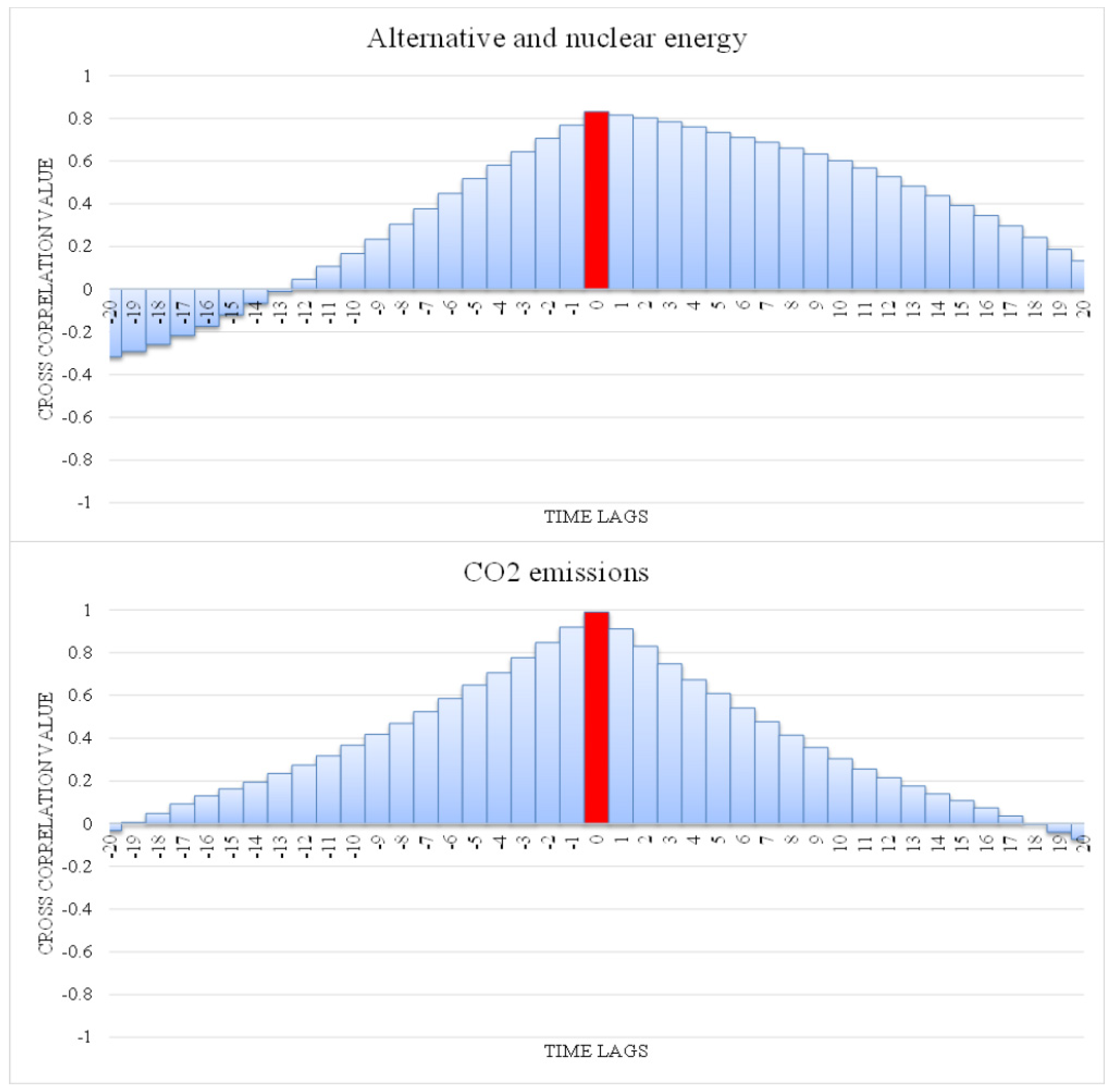
3.1.2. Data Preprocessing (Feature Selection, Lag Selection and Data Normalization)

In machine learning problems, it is very challenging to select a representative collection of features to build the model [94]. Studying more features (a larger feature set), helps to explore more problem dimensions and to reduce the threat of missing potential solutions, but at the same time it may conclude more computational complexity, learning algorithm confusing, and over learning.

DM, as a process, generally contains data cleaning, integration, selection and transformation to discover patterns, evaluate them, and present the extracted knowledge [103,119]. In knowledge discovery processes, such as DM, the feature subset selection is very crucial, not only for the insight achieved from determining variables, but also for the upgraded reprehensibility, scalability, and the validity of the constructed models [13]. This research uses a correlation-based feature selection (CFS) algorithm to determine the most relevant input features. CFS was initially proposed by Hall in 1999 [94]. A CFS examines and ranks feature subsets, unlike many much-used techniques which aimed to rank features individually, such as ReliefF [120]. CFS consists of two nested steps: (1) feature evaluation and (2) searching the feature subset [95].

The feature evaluation step is the heart of a CFS which aimed to heuristically measure the merit of a subset of features. This process studies the usefulness of every single feature to predict targeted variable (here natural gas consumption) while the inter-correlation level among subset is investigated. Equation (1) formulizes this heuristic, proposed by Ghiselli [121] which is a form of Pearson’s correlation, where all variables are standardized.

$$Meri{t}_S=\frac{k \overline{r_{cf}}}{\sqrt{k+\left(k-1\right)\overline{r_{ff}}}}$$

(1)

where the equation aimed to evaluate merit of a feature subset S composed of k features. $\overline{r_{cf}}$ represents the average feature-class correlation and $\overline{r_{ff}}$ refers to the average feature-feature inter-correlation.

To decide which of the features to include in the final subset and which to ignore one would try all possible subsets. Note that for k possible features there are 2^k possible subsets. Obviously, it is not a logical procedure to investigate all possible subsets one by one especially when k is relatively large. To address this challenge various heuristic search strategies are proposed which often converge to an optimal subset in reasonable time [95,122]. "Best First" [123] and "Greedy Stepwise" [124] searching methods were applied to the CFS to study input dataset using various searching paradigms. For instance, the best first starts with an empty set and develops all possible single feature subsets. The subset with the highest evaluation value, as noted above, selected to expand by adding another single feature. The stopping condition is obtained when expanding the subset results in no improvement. Both of searching methods resulted in the same feature subset which means they support each other. Finally, through 13 representative input features (presented in Table 3) six input features selected as the model’s input, contains: (1) alternative and nuclear energy, (2) CO₂ emissions, (3) GDP per capita, (4) urban population, (5) NG production, and (6) oil consumption.

Sometimes relevant features in a time series dataset show their influence with lags of time. Also, there would be time lags for a policy/decision in the complex energy market. Detecting related lags would assist a prediction model to accurately follow possible fluctuations [17]. At this step, the proposed DmGNn methodology attempts to determine time lags related to finalized feature subset correlated with the target attribute (i.e., NG global demand).

Numerous lag selection approaches exist that contain lag selection as a pre-processing, post-processing, or even as a part of the learning process [125]. Among popular statistical tests based on information criteria pre-processing lag selection methods, Akaike information criteria (AIC), Bayesian information criteria (BIC), and Schwarz Bayesian information criteria (SBIC), are well used [126,127]. Information criteria methods consider 1 lag (as the minimum number) to p which define intermediate lags. The main hypothesis is to define the lag order p to minimize the following equation:

$$IC\left(p\right)=Nln\widehat{{\sigma }^2}\left(p\right)+p\left[f\left(N\right)\right]$$

(2)

where $\widehat{{\sigma }^2}\left(p\right)$ is defined as the estimated regression variance, related to the sample size and order p of lag structure, and N is the number of observations [128]. $p\left[f\left(N\right)\right]$ is the penalty function to increase the order of model. Different choices of $f\left(N\right)$ cause in different information criteria.

A −20 to +20 time lags were implemented for each feature versus the target attribute using Matlab software. Figure 2 summarizes results of the time lag selection process for selected features, alternative and nuclear energy and CO₂ emissions. For each chart, the vertical axis shows the level of correlation between the correspondence feature and targeted variable while horizontal axis implies different time lags. The order p defines the effective time lag which possess the highest correlation level, according to the chart.

Now, optimum input features are detected. Six selected features are representatives of all 13 identified input features and also the selected subset has been reorganized based on detected time lags.

Although an optimum set of input features have been selected, still input features are asymmetric and the units are different in scales. Data normalization step is investigated to restrain the parameters range influence on the results and adapt values of different features with different domains and scales to a shared scale. The min-max normalization method is used to adjust dataset using the following equation:

$$Normalized Data=\frac{y\left(i\right)-\min \left\{y\right\}}{max\left\{y\right\}-\min \left\{y\right\}}$$

(3)

where y(i) is an ith element in the column and $min\left\{y\right\}$ minimum and $max\left\{y\right\}$ is the maximum of related column’s elements.

The next sub-section is dedicated to discussing the forecasting framework.

3.2. Designing the Forecasting Framework

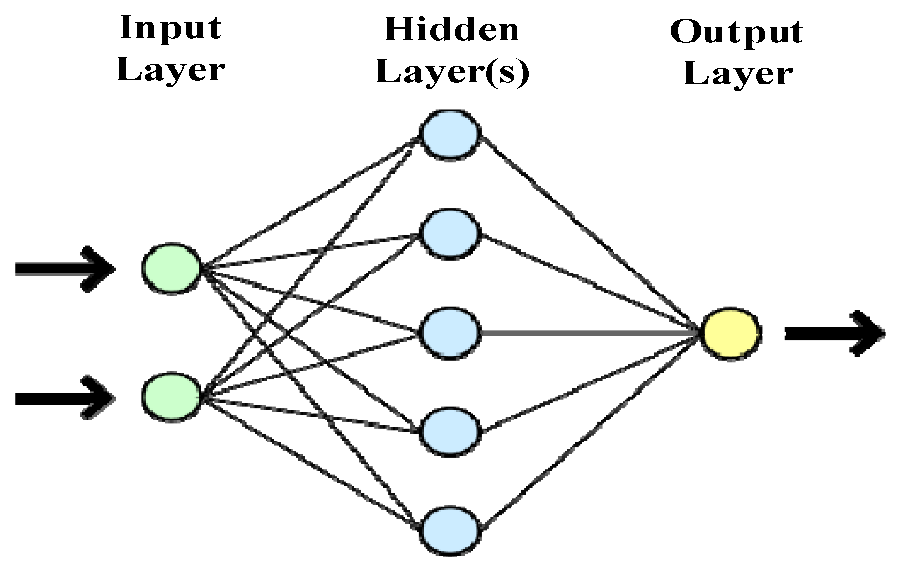
3.2.1. Artificial Neural Network

Computational intelligence methods such as an artificial neural network (ANNs) [129] are modern paradigms to handle complex optimization problems [130,131,132]. ANN is organized as a simplified abstract of the biological nervous system to emulate neurons mechanism. A neuron is the computation unit of an ANN. Mathematically a neuron is a function, which aimed at dynamically reduce deviation cost. The mathematical description of a neuron presented as follows:

$$O_j\left(t\right)=f\left\{\left[{\displaystyle \sum }_{i=1}^n{w}_{ij}{x}_i\left(t-{\tau }_{ij}\right)\right]-T_j\right\}$$

(4)

where x_i and o_j respectively are the input and the output at time t, ${\tau }_{ij}$ defines the delay between x_i and o_j. T_j presents the threshold of the jth neuron, while w_ij is the connection coefficient from neuron i to neuron j.

An ANN consists of characteristics: the input layer, the hidden layer, the interconnection between different layers, the learning step to find the optimum values of interconnections weights, the transformer function which assigned to produce outputs refer to weighted inputs, the number of neurons performing in each layer and the output layer. Figure 3 schematically presents the architecture of an ANN with a single hidden layer.

As it has been shown in Figure 3, neurons are deployed in layers. Nodes of layers in a row are connected to show interactions and information flow in an ANN. The connection between node i and j defines by the weight w_ij and also a bias b_i parameter is assigned to each neuron [133]. To minimize the error at each step (which is known as epoch) an ANN compute and error function and uses an algorithm to reduce the error value.

An ANN has the ability to be trained in order to build a precise network and minimize the lost function by adjusting w_ij weight matrices [17]. So, the performance of the learning algorithm will define the performance of the ANN. In this paper, a genetic algorithm (GA) is used to equip ANN as the learning algorithm. In the next section, the GA procedure is explained briefly.

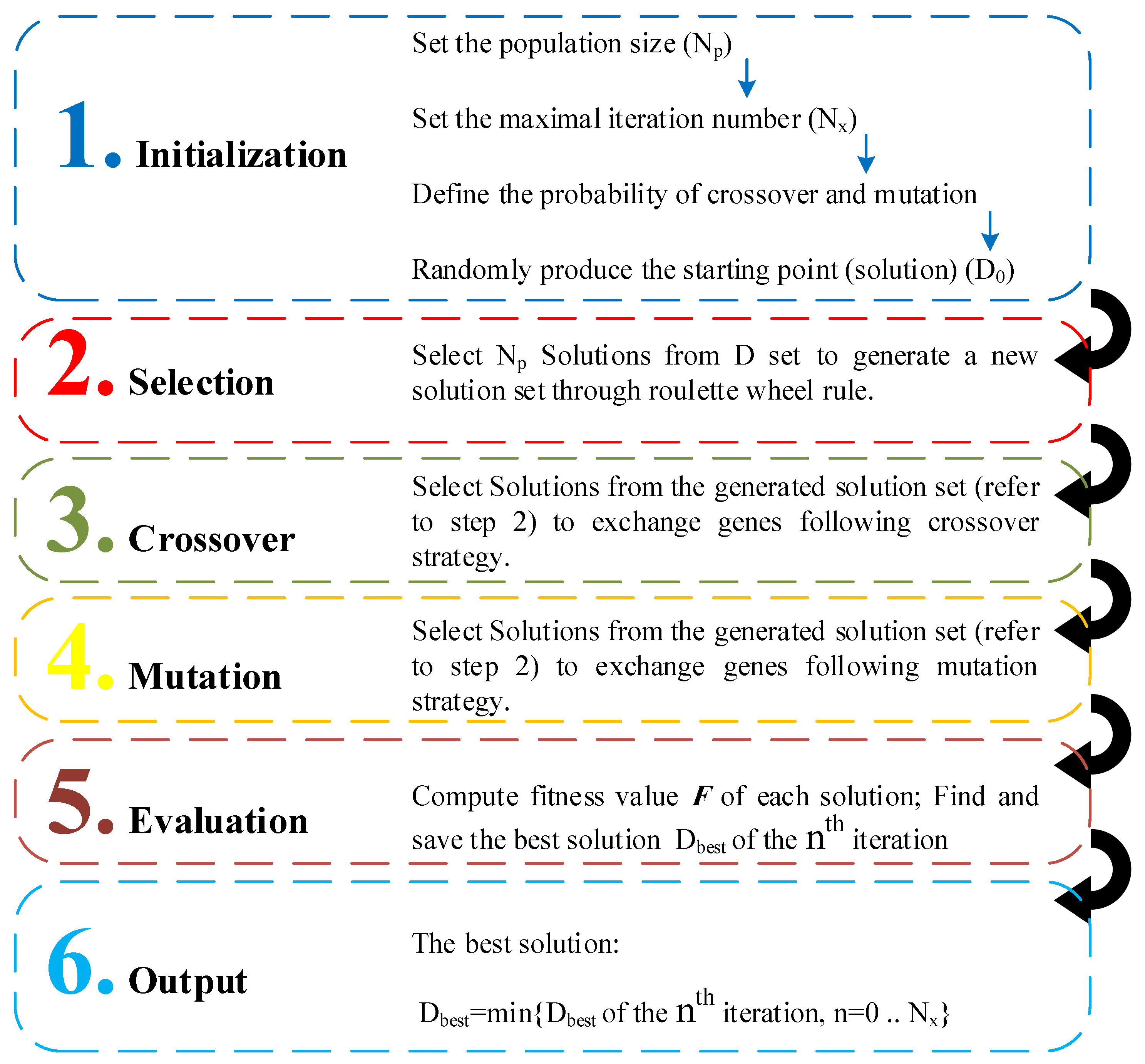
3.2.2. Genetic Algorithm

Training an ANN is very complex, which can directly influence outcomes’ quality. Recently, numerous academic studies are presented, which applied meta-heuristic and intelligent algorithms (i.e., GA) as learning algorithms [134].

GA is an evolutionary optimization approach developed by Holland in 1975 [101], which acts based on random search procedure. Compared to traditional optimization methods the GA has numerous advantages. For example, the algorithm converges to a good, feasible solution faster than other existing traditional methods [24]. Series of computational operators like selection, mutation, and crossover functions are used in a GA to achieve a reliable solution. Figure 4 briefly presents the GA procedure.

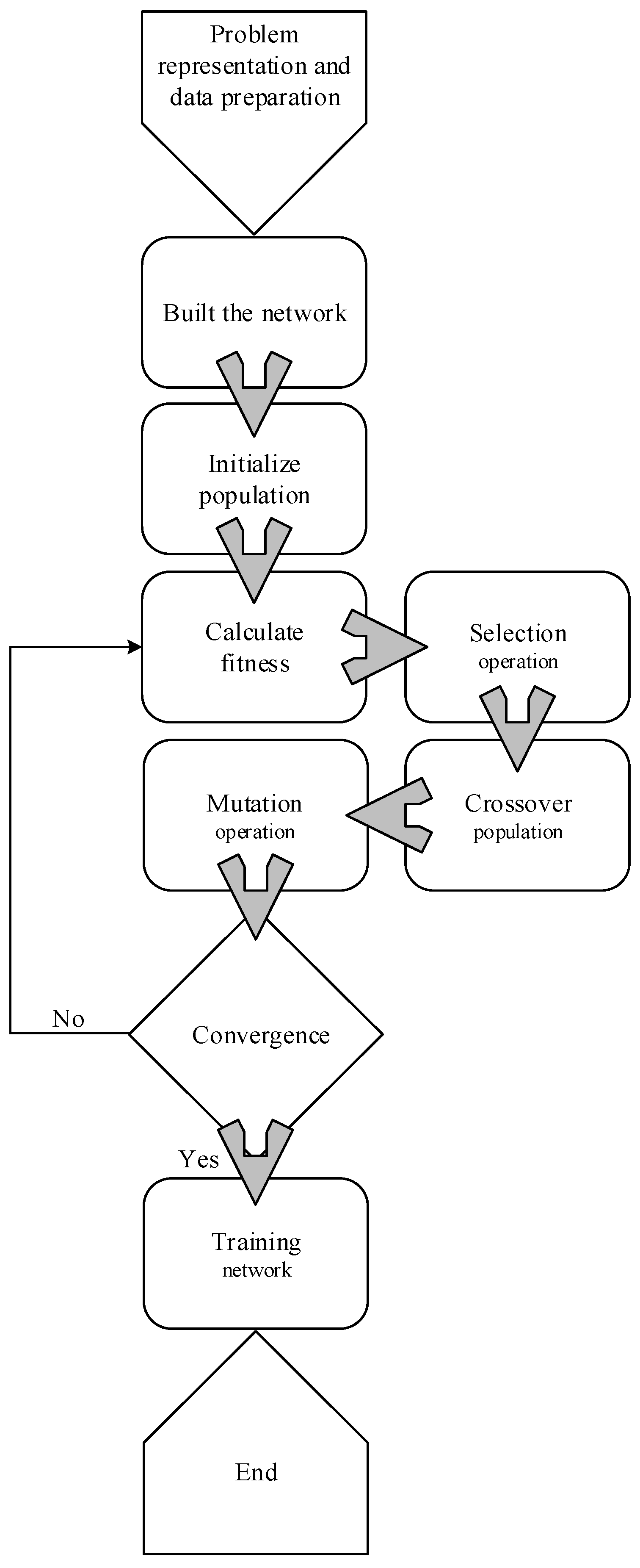
3.2.3. Genetic Neural Network

In this paper, weights and thresholds of the ANN are updated by a GA. For this purpose, input vectors transformed into a genetic gene in the format of the chromosome. Then, the initial population is formed from the randomly generated chromosome. Now values of the optimization algorithm such as selection, crossover, and mutation rates can be set to design the algorithm. The fitness function is the reciprocal of the quadratic sum of the difference between predicted and real values [135]. Roulette wheel selection is used to select a new individual, then two chromosomes are exchanged via crossover operation to generate a new individual. Finally, the mutation step is applied to avoid premature convergence.

Equipping an ANN with a GA could save training time and improve the precision of the forecasting model [135]. Figure 5 schematically shows the flowchart of the presented GNN.

The next section is dedicated to present the architecture of ANN, which is the basic framework of the developed forecasting model.

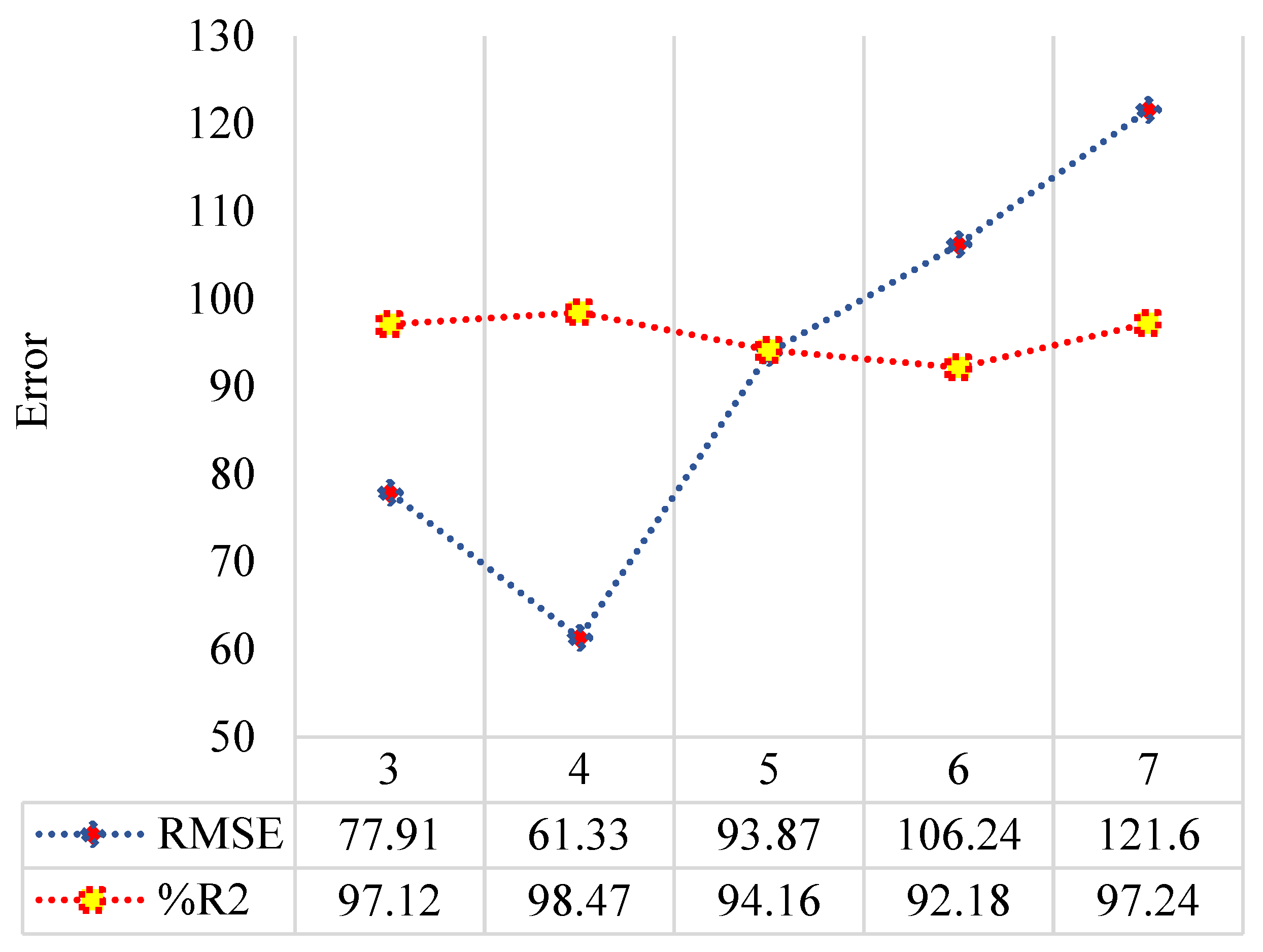
3.2.4. The Architecture of the ANN

This research targeted to present accurate NG demand predictions, so the selected features were inputted at the initiatory layer (input layer) of the designed ANN. A single hidden layer network was designed to perform the prediction, so the model contains a three-layer architecture. Figure 6 shows the performance of a three-layered NN for three, four, five, six, and seven neurons in the hidden layer. Four neurons were used for the hidden layer as it returns the best performance among other tested number of neurons (see Figure 6).

As it has been represented in Figure 6, based on the R² and root mean square error (RMSE) statistics, four number of neurons the proposed data mining genetic-neural network (DmGNn) model performs better than other examined set.

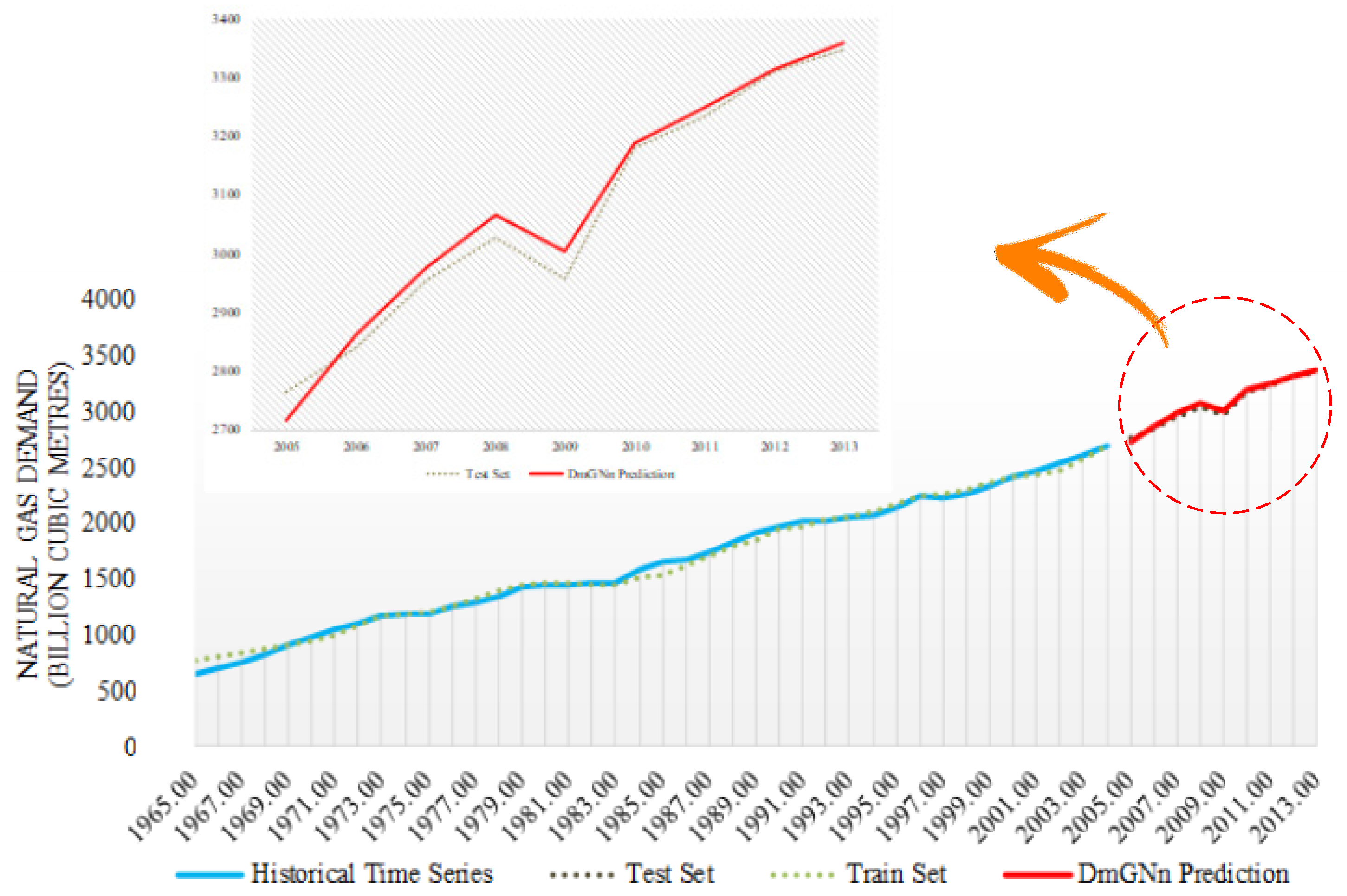
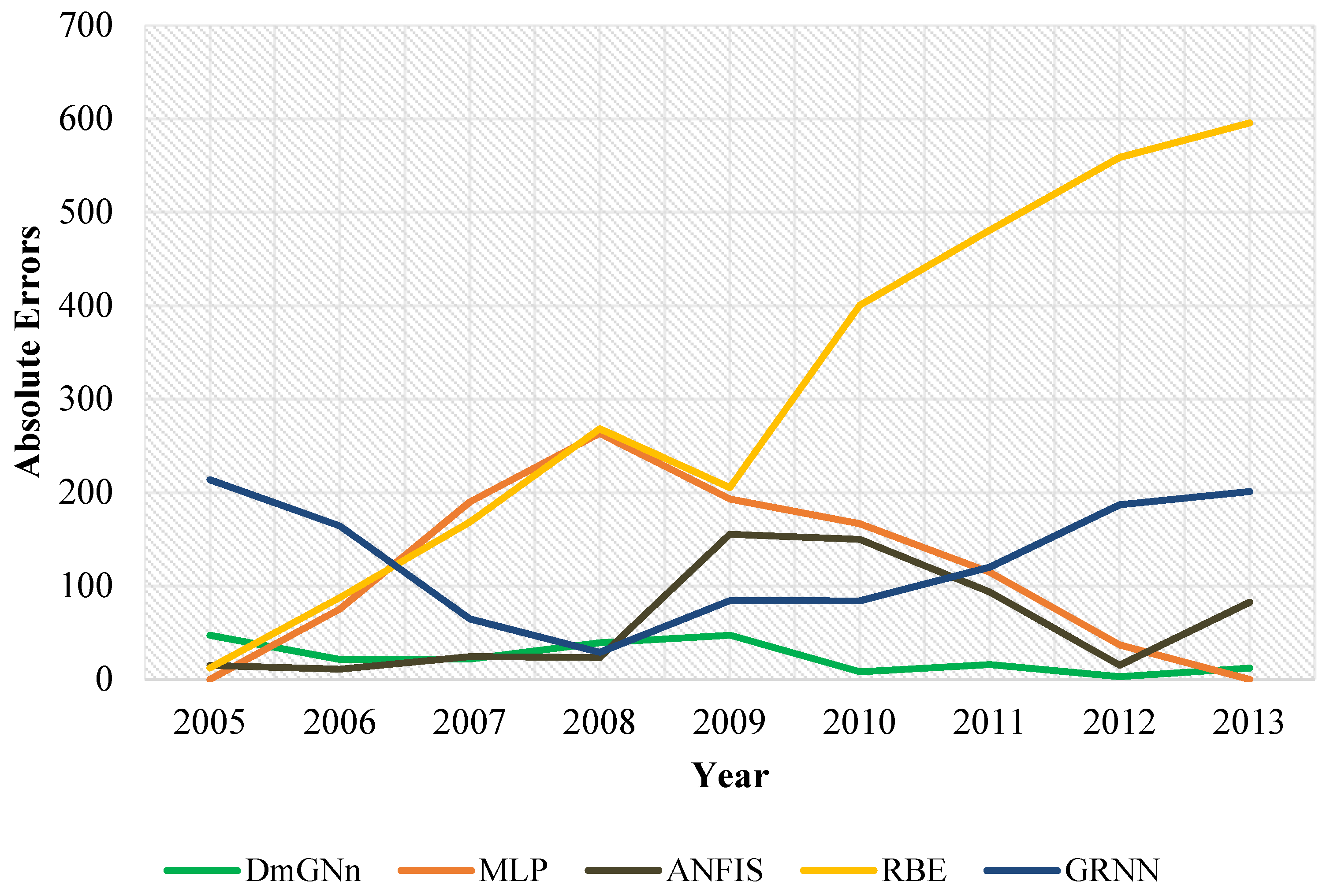
4. Outputs and Results

As mentioned before this paper is aimed at developing a forecasting model to accurately forecast global NG demand. Here, the historical behavior of the global NG demand from 1965 to 2013 period (billion cubic meters) is gathered via www.bp.com. Now, the model is designed, and it can be used to project future trends for NG global consumption. For this reason, 40 historical annual fundamental time series data (from 1665 to 2004) are investigated as a learning set. The forecasting period contains nine annual values for NG global demand prediction problem (from 2005 to 2013). Ten iterations have been investigated for the proposed DmGNn model. Figure 7 presents projections (average for 10 iterations) resulted from the DmGNn models.

Learning models were extensively applied in the case of NG demand predictions [62,136]. Some competitive prediction models were selected to compare outputs of the proposed model and analysis of the accuracy. Adaptive Neuro-Fuzzy Inference Systems (ANFIS) [137,138,139] and a set of classical well-known neural network-based techniques such as: Radial Basis Function Neural Network (RBF) [140,141], Multi-Layered Perceptron (MLP) [18,142], and Generalized Regression Neural Network (GRNN) [143,144,145] are nominated and optimized (through trial and error processes to minimize forecast errors) to prove the accuracy of the proposed DmGNn model through a comparison study.

To evaluate different models, a set of mathematical criteria organized to measure prediction performance. A relatively large set of validity indicators support the justification of model usage [21]. These statistics are summarized in

Table 4. Used mathematical criteria to evaluate forecast errors.

Error Title	Abbreviation	Formula
R-squared	R2	${\mathrm{R}}^2=1-\frac{S{S}_{res}}{S{S}_{tot}}$ *
Mean Absolute Error	MAE	$\mathrm{MAE}=\frac{1}{n}{\displaystyle {\displaystyle \sum }_i}\left|f_i-y_i\right|$
Mean Absolute Percentage Error	MAPE	$\mathrm{MAPE}=\frac{100}{n}{\displaystyle {\displaystyle \sum }_i}\left|\frac{f_i-y_i}{y_i}\right|$
Mean Bias Error	MBE	$\mathrm{MBE}=\frac{1}{n}{\displaystyle {\displaystyle \sum }_i}\left(f_i-y_i\right)$
Root Mean Square Error	RMSE	$\mathrm{RMSE}=\sqrt{\frac{{\displaystyle \sum }{\left(y_i-f_i\right)}^2}{n}}$

* Where, $S{S}_{tot}={{\displaystyle \sum }}_i{\left(y_i-\overline{y}\right)}^2$ and $S{S}_{res}={{\displaystyle \sum }}_i{\left(y_i-f_i\right)}^2={{\displaystyle \sum }}_i{\left(errors\right)}^2$.

(where y_i refers to real historical value and f_i presents forecasting value).

Each model ran for 10 times and the average of outputs was calculated.

Table 5. Statistical errors for each prediction model.

Models	Characteristics	R2	MAE	MAPE	MBE	RMSE
DmGNn	Number of Neurons = 4; Maximum generation = 100; Cross Over Probability = 0.8; Mutation Probability = 0.05;	0.9847	52.19	1.69	13.54	61.33
MLP	Maximum Epochs = 200; Train Parameter Goal = 1 × 10−7;	0.8241	115.59	3.80	−44.85	145.61
ANFIS	FIS Generation Approach: FCM; Number of Clusters = 10; Partition Matrix exponent = 2;	0.8494	63.45	1.89	21.31	84.31
RBF	Spread Value = 0.17;	0.0018	308.64	10.42	−308.64	366.51
GRNN	Spread Value = 1;	0.9864	127.63	4.17	−4.03	142.12

presents the performance of the proposed and competitive models refer to statistics introduced in Table 4.

As it is shown in Table 5, the proposed DmGNn significantly outperforms other competitive models. Although the GRNN presents a reasonable performance under R² (for R² both DmGNn and GRNN almost performed similar) and MBE criteria, however, it failed under MAE and RMSE error tests. Here multiple error tests have been implemented to show estimators’ accuracy comprehensively. Among them, MAE and RMSE are mentioned and used by many previous researchers and claimed that the combination of MAE and RMSE could be more beneficial [146]. The RMSE is more appropriate to represent model performance than the MAE when the error distribution is expected to be Gaussian [146]. Simultaneously, Willmott and Matsuura suggested that the RMSE is not a good indicator of average model performance and might be a misleading indicator of average error, and, thus, the MAE would be a better metric for that purpose [147]. The DmGNn overcame other competitive models under both RMSE and MAE.

The pattern of the absolute error for each model is shown in Figure 8, which represents how various forecasting models behave along the test period. As it is shown, the proposed DmGNn outperforms other benchmark forecasting models (with lower absolute error value for forecasting period) and resulted in a robust forecast series (unlike other forecasting models DmGNn’s forecast errors showed a low swing pattern).

Table 5 and Figure 8 showed how the proposed DmGNn model overcame other benchmark models. However, the initial objective was to propose a prediction model which is aimed to uncover main driving forces in order to approach to reliable extrapolations. ANN and GA were combined and implemented successfully by other previous researchers to predict future trends in the area of energy (for instance: [40,58,65,67,69]), but this paper presents a GNn with adjusted characteristics equipped with a purified input vector using data mining based pre-processing techniques. Data mining significantly helped to improve prediction accuracy and reliability. To show the efficiency of the data mining phases, both pre-processed and raw data were applied to the design prediction model.

Table 6. Statistical errors for different input vectors (raw versus processed).

Input Protocol	R2	MAE	MAPE	MBE	RMSE
Processed data	0.9847	52.19	1.69	13.54	61.33
Raw data	0.9679	79.96	2.61	2.66	94.21

compared the results under statistical errors criteria.

As it has been shown, even the GRNN with a purified input vector overcame the GNn in the case of R² indicator (0.9864 > 0.9679). Moreover, to dedicate a better understanding, Figure 9 shows absolute error for two different input protocols (purified using data mining and raw data) along the testing period. The line related to GNn represents more fluctuations than the green line (belongs to DmGNn), simultaneously shows a larger number for errors corresponding to each test point (years).

5. Conclusions

Energy is a major topic both in practice and theory, which many researchers investigated issues related to energy sectors and industries. The international energy supply system is characterized by a complicated combination of technological, social, economic, and political elements. Predicting and planning for the future global energy market is interesting and, simultaneously, a challenging subject in both research and practical investment projects. Thus the accurate prediction of energy demand is critical to developing future policies, modify current plans, and evaluate potential strategies since the energy market are complex and changing dynamically over time. This paper primary targeted to provide an accurate and robust prediction model to predict the global natural gas demands using a learning-based prediction model. On the other hand, authors aimed at introducing a process which reduces problem space dimensions to define the most relevant features subset which affects NG future consumption trends. The subset contains input features which shape the future, which are defined as driving forces. The estimator model can predict trends easier as the input is purified and the adjusted input vector has fewer dimensions than raw input vector, and also policymakers can monitor or in some cases manipulate NG market refers to extracted features.

In order to investigate maximum feasible solutions and to prevent missing any potential optimal option, input features were gathered based on the literature review and also related online dataset survey. Input features would define the model structure and support the accuracy of the output results. Although, increasing the number of input variables may cause computational complexity and reducing interpretability of the results. Instead, a large number of input features expands solution space and consequently reduces the probability of ignoring appropriate answers. A feature selection step is proposed and is implemented to reduce the dataset dimensions while guarantees that the prediction model will explore all optimal solutions. Finally, six input features were selected among 13 primary input features. The feature selection approach guarantees to investigate all solution space using a limited set of input features. Then possible time lags among input features versus the targeted attribute (NG global demand) were studied and subsequently applied to the refined input set. Investigating suitable time lags will cause in a more accurate and rational prediction model, which guarantees synchronization between input features and the target attribute at t time step. Finally, a neural network framework is developed, which equipped using a genetic algorithm to optimize the network’s characteristics aimed to predict future NG global demands.

Four benchmark models are investigated to study the performance of the proposed data mining genetic-neural network (DmGNn) model. The proposed DmGNn model outperforms other benchmark models refer to five different error statistics. Based on the R² statistic the DmGNn track real testing set fluctuations very well (only missed about 2%). Moreover, to distinct how the proposed pre-processing step affects the model accuracy, DmGNn model compared to a single GNn (without pre-processing phases). As shown the proposed pre-processing step improves predictions both in term of accuracy and reliability (robustness). Moreover, based on the interpretative capability index, the DmGNn dedicates a more clear vision about future trends since it uses a smaller input dataset. A limited input feature set enables decision-makers to design responsive policies/strategies/actions as they were aware of attributes affecting the global NG demands.

The proposed DmGNn is characterized by high flexibility, universal operation, learning ability, and low requirements for computation resources. As a result, it can be used by decision-makers and market participants who face a complex environment. Although results showed notably high-performance indexes for the proposed DmGNn model but such mathematical models are limited to conditions where appropriate and reliable data is provided. Moreover, in the conditions of availability of data mathematical estimators, even learning-based, are constrained to the historical time series and emerging signals with no significant background are neglected and subsequently and can cause deviation in the predictions. For further studies, a hybrid qualitative-quantitative model can be considered in order to cover a single quantitative prediction model’s weaknesses.

References

1. BP. Statistical Review of World Energy; BP: London, UK, 2016. [Google Scholar]
2. IEA. World Energy Outlook; IEA: Paris, France, 2016. [Google Scholar]
3. EIA. Annual Energy Outlook; EIA: Paris, France, 2017.
4. Alipour, M.; Hafezi, R.; Ervural, B.; Kaviani, M.A.; Kabak, O. Long-term policy evaluation: Application of a new robust decision framework for Iran’s energy exports security. Energy 2018, 157, 914–931. [Google Scholar] [CrossRef]
5. EIA. Annual Energy Outlook; EIA: Paris, France, 2016.
6. Hafezi, R.; Akhavan, A.; Pakseresht, S. Projecting plausible futures for Iranian oil and gas industries: Analyzing of historical strategies. J. Nat. Gas Sci. Eng. 2017, 39, 15–27. [Google Scholar] [CrossRef]
7. Alipour, M.; Hafezi, R.; Amer, M.; Akhavan, A.N. A new hybrid fuzzy cognitive map-based scenario planning approach for Iran’s oil production pathways in the post-sanction period. Energy 2017, 135, 851–864. [Google Scholar] [CrossRef]
8. Hafezi, R.; Akhavan, A.; Pakseresht, S. The State of Competition in Natural gas Market Application of Porter’s Five Forces for NIGC, In Proceedings of the International Gas Union Research Conference (IGRC), Rio de Janeiro, Brazil, 24–26 May 2017.
9. Hafezi, R.; Bahrami, M.; Akhavan, A.N. Sustainability in development: Rethinking about old paradigms. World Rev. Sci. Technol. Sustain. Dev. 2017, 13, 192–204. [Google Scholar] [CrossRef]
10. Hafezi, R.; Akhavan, A.N.; Pakseresht, S.; Wood, D.A. A Layered Uncertainties Scenario Synthesizing (LUSS) model applied to evaluate multiple potential long-run outcomes for Iran’s natural gas exports. Energy 2019, 169, 646–659. [Google Scholar] [CrossRef]
11. Alipour, M.; Alighaleh, S.; Hafezi, R.; Omranievardi, M. A new hybrid decision framework for prioritizing funding allocation to Iran’s energy sector. Energy 2017, 121, 388–402. [Google Scholar] [CrossRef]
12. Gheyas, I.A.; Smith, L.S. Feature subset selection in large dimensionality domains. Pattern Recognit. 2010, 43, 5–13. [Google Scholar] [CrossRef] [Green Version]
13. Kim, Y.; Street, W.N.; Menczer, F. Feature selection in data mining. Data Min. Oppor. Chall. 2003, 3, 80–105. [Google Scholar]
14. Guyon, I.; Elisseeff, A. An introduction to variable and feature selection. J. Mach. Learn. Res. 2003, 3, 1157–1182. [Google Scholar]
15. Koller, D.; Sahami, M. Toward Optimal Feature Selection; Stanford InfoLab: Stanford, CA, USA, 1996. [Google Scholar]
16. Bishop, C.M. Pattern Recognition and Machine Learning; Springer: Berlin, Germany, 2006. [Google Scholar]
17. Hafezi, R.; Shahrabi, J.; Hadavandi, E. A bat-neural network multi-agent system (BNNMAS) for stock price prediction: Case study of DAX stock price. Appl. Soft Comput. 2015, 29, 196–210. [Google Scholar] [CrossRef]
18. Hafezi, R.; Akhavan, A.N. Forecasting Gold Price Changes: Application of an Equipped Artificial Neural Network. AUT J. Model. Simul. 2018, 50, 71–82. [Google Scholar]
19. Kourou, K.; Exarchos, T.P.; Exarchos, K.P.; Karamouzis, M.V.; Fotiadis, D.I. Machine learning applications in cancer prognosis and prediction. Comput. Struct. Biotechnol. J. 2015, 13, 8–17. [Google Scholar] [CrossRef]
20. Dessì, D. A Recommender System of Medical Reports Leveraging Cognitive Computing and Frame Semantics, in Machine Learning Paradigms; Springer: Berlin, Germany, 2019; pp. 7–30. [Google Scholar]
21. Panapakidis, I.P.; Dagoumas, A.S. Day-ahead natural gas demand forecasting based on the combination of wavelet transform and ANFIS/genetic algorithm/neural network model. Energy 2017, 118, 231–245. [Google Scholar] [CrossRef]
22. Kazemi, S.; Hadavandi, E.; Mehmanpazir, F.; Nakhostin, M. A hybrid intelligent approach for modeling brand choice and constructing a market response simulator. Knowl. Based Syst. 2013, 40, 101–110. [Google Scholar] [CrossRef]
23. Júnior, S.E.R.; de Oliveira Serra, G.L. A novel intelligent approach for state space evolving forecasting of seasonal time series. Eng. Appl. Artif. Intell. 2017, 64, 27–285. [Google Scholar]
24. Ervural, B.C.; Beyca, O.F.; Zaim, S. Model Estimation of ARMA Using Genetic Algorithms: A Case Study of Forecasting Natural Gas Consumption. Procedia Soc. Behav. Sci. 2016, 235, 53–545. [Google Scholar] [CrossRef]
25. Zhu, L.; Li, M.S.; Wu, Q.H.; Jiang, L. Short-term natural gas demand prediction based on support vector regression with false neighbours filtered. Energy 2015, 80, 428–436. [Google Scholar] [CrossRef]
26. Xu, N.; Dang, Y.; Gong, Y. Novel grey prediction model with nonlinear optimized time response method for forecasting of electricity consumption in China. Energy 2016, 118, 473–480. [Google Scholar] [CrossRef]
27. Bianco, V.; Scarpa, F.; Tagliafico, L.A. Scenario analysis of nonresidential natural gas consumption in Italy. Appl. Energy 2014, 113, 392–403. [Google Scholar] [CrossRef]
28. Baldacci, L.; Golfarelli, M.; Lombardi, D.; Sami, F. Natural gas consumption forecasting for anomaly detection. Expert Syst. Appl. 2016, 62, 190–201. [Google Scholar] [CrossRef]
29. Zavanella, L.; Zanoni, S.; Ferretti, I.; Mazzoldi, L. Energy demand in production systems: A Queuing Theory perspective. Int. J. Prod. Econ. 2015, 170, 393–400. [Google Scholar] [CrossRef]
30. Baumeister, C.; Kilian, L. Real-time analysis of oil price risks using forecast scenarios. IMF Econ. Rev. 2011, 62, 119–145. [Google Scholar] [CrossRef]
31. Dilaver, Ö.; Dilaver, Z.; Hunt, L.C. What drives natural gas consumption in Europe? Analysis and projections. J. Nat. Gas Sci. Eng. 2014, 19, 125–136. [Google Scholar] [CrossRef]
32. Li, J.; Dong, X.; Shangguan, J.S.; Hook, M. Forecasting the growth of China’s natural gas consumption. Energy 2011, 36, 1380–1385. [Google Scholar] [CrossRef]
33. Suganthi, L.; Samuel, A.A. Energy models for demand forecasting—A review. Renew. Sustain. Energy Rev. 2012, 16, 1223–1240. [Google Scholar] [CrossRef]
34. Aras, H.; Aras, N. Forecasting residential natural gas demand. Energy Sources 2004, 26, 463–472. [Google Scholar] [CrossRef]
35. Erdogdu, E. Natural gas demand in Turkey. Appl. Energy 2010, 87, 211–219. [Google Scholar] [CrossRef] [Green Version]
36. Gori, F.; Ludovisi, D.; Cerritelli, P. Forecast of oil price and consumption in the short term under three scenarios: Parabolic, linear and chaotic behaviour. Energy 2007, 32, 1291–1296. [Google Scholar] [CrossRef]
37. Kumar, U.; Jain, V. Time series models (Grey-Markov, Grey Model with rolling mechanism and singular spectrum analysis) to forecast energy consumption in India. Energy 2010, 35, 1709–1716. [Google Scholar] [CrossRef]
38. Akkurt, M.; Demirel, O.F.; Zaim, S. Forecasting Turkey’s natural gas consumption by using time series methods. Eur. J. Econ. Political Stud. 2010, 3, 1–21. [Google Scholar]
39. Sen, P.; Roy, M.; Pal, P. Application of ARIMA for forecasting energy consumption and GHG emission: A case study of an Indian pig iron manufacturing organization. Energy 2016, 116, 1031–1038. [Google Scholar] [CrossRef]
40. Fagiani, M.; Squartini, S.; Gabrielli, L.; Spinsante, S. A review of datasets and load forecasting techniques for smart natural gas and water grids: Analysis and experiments. Neurocomputing 2015, 170, 448–465. [Google Scholar] [CrossRef]
41. Shi, G.; Liu, D.; Wei, Q. Energy consumption prediction of office buildings based on echo state networks. Neurocomputing 2016, 216, 478–488. [Google Scholar] [CrossRef]
42. Zhang, W.; Yang, J. Forecasting natural gas consumption in China by Bayesian model averaging. Energy Rep. 2015, 1, 216–220. [Google Scholar] [CrossRef]
43. Taşpınar, F.; Celebi, N.; Tutkun, N. Forecasting of daily natural gas consumption on regional basis in Turkey using various computational methods. Energy Build. 2013, 56, 23–31. [Google Scholar] [CrossRef]
44. Dalfard, V.M.; Asli, M.N.; Asadzadeh, S.M.; Sajjadi, S.M.; Nazari-Shirkouhi, A. A mathematical modeling for incorporating energy price hikes into total natural gas consumption forecasting. Appl. Math. Model. 2013, 37, 5664–5679. [Google Scholar] [CrossRef]
45. Bianco, V.; Scarpa, F.; Tagliafico, L.A. Analysis and future outlook of natural gas consumption in the Italian residential sector. Energy Convers. Manag. 2014, 87, 754–764. [Google Scholar] [CrossRef]
46. Gorucu, F. Evaluation and forecasting of gas consumption by statistical analysis. Energy Sour. 2004, 26, 267–276. [Google Scholar] [CrossRef]
47. O’Neill, B.C.; Desai, M. Accuracy of past projections of US energy consumption. Energy Policy 2005, 33, 979–993. [Google Scholar] [CrossRef] [Green Version]
48. Adams, F.G.; Shachmurove, Y. Modeling and forecasting energy consumption in China: Implications for Chinese energy demand and imports in 2020. Energy Econ. 2008, 30, 1263–1278. [Google Scholar] [CrossRef]
49. Ramanathan, R. A multi-factor efficiency perspective to the relationships among world GDP, energy consumption and carbon dioxide emissions. Technol. Forecast. Soc. Chang. 2006, 73, 483–494. [Google Scholar] [CrossRef]
50. Lu, W.; Ma, Y. Image of energy consumption of well off society in China. Energy Convers. Manag. 2004, 45, 1357–1367. [Google Scholar] [CrossRef]
51. Hunt, L.C.; Ninomiya, Y. Primary energy demand in Japan: An empirical analysis of long-term trends and future CO 2 emissions. Energy Policy 2005, 33, 1409–1424. [Google Scholar] [CrossRef]
52. Iniyan, S.; Suganthi, L.; Samuel, A.A. Energy models for commercial energy prediction and substitution of renewable energy sources. Energy Policy 2006, 34, 2640–2653. [Google Scholar] [CrossRef]
53. Sözen, A.; Arcaklioğlu, E.; Özkaymak, M. Turkey’s net energy consumption. Appl. Energy 2005, 81, 209–221. [Google Scholar] [CrossRef]
54. Ermis, K.; Midilli, A.; Dincer, I.; Rosen, M.A. Artificial neural network analysis of world green energy use. Energy Policy 2007, 35, 1731–1743. [Google Scholar] [CrossRef]
55. Sözen, A.; Arcaklioglu, E. Prediction of net energy consumption based on economic indicators (GNP and GDP) in Turkey. Energy Policy 2007, 35, 4981–4992. [Google Scholar] [CrossRef]
56. Sözen, A.; Gülseven, Z.; Arcaklioğlu, E. Forecasting based on sectoral energy consumption of GHGs in Turkey and mitigation policies. Energy Policy 2007, 35, 6491–6505. [Google Scholar] [CrossRef]
57. Geem, Z.W.; Roper, W.E. Energy demand estimation of South Korea using artificial neural network. Energy Policy 2009, 37, 4049–4054. [Google Scholar] [CrossRef]
58. Forouzanfar, M.; Doustmohammadi, A.; Menhaj, M.B.; Hasanzadeh, S. Modeling and estimation of the natural gas consumption for residential and commercial sectors in Iran. Appl. Energy 2010, 87, 268–274. [Google Scholar] [CrossRef]
59. Ekonomou, L. Greek long-term energy consumption prediction using artificial neural networks. Energy 2010, 35, 512–517. [Google Scholar] [CrossRef] [Green Version]
60. Rodger, J.A. A fuzzy nearest neighbor neural network statistical model for predicting demand for natural gas and energy cost savings in public buildings. Expert Syst. Appl. 2014, 41, 1813–1829. [Google Scholar] [CrossRef]
61. Aydinalp-Koksal, M.; Ugursal, V.I. Comparison of neural network, conditional demand analysis, and engineering approaches for modeling end-use energy consumption in the residential sector. Appl. Energy 2008, 85, 271–296. [Google Scholar] [CrossRef]
62. Aramesh, A.; Montazerin, N.; Ahmadi, A. A general neural and fuzzy-neural algorithm for natural gas flow prediction in city gate stations. Energy Build. 2014, 72, 73–79. [Google Scholar] [CrossRef]
63. Szoplik, J. Forecasting of natural gas consumption with artificial neural networks. Energy 2015, 85, 208–220. [Google Scholar] [CrossRef]
64. Soldo, B.; Potocnik, P.; Simunovic, G.; Saric, T.; Govekar, E. Improving the residential natural gas consumption forecasting models by using solar radiation. Energy Build. 2014, 69, 498–506. [Google Scholar] [CrossRef]
65. Izadyar, N.; Ong, H.C.; Shamshirband, S.; Ghadamian, H.; Tong, C.W. Intelligent forecasting of residential heating demand for the District Heating System based on the monthly overall natural gas consumption. Energy Build. 2015, 104, 208–214. [Google Scholar] [CrossRef]
66. González-Romera, E.; Jaramillo-Morán, M.Á.; Carmona-Fernández, D. Forecasting of the electric energy demand trend and monthly fluctuation with neural networks. Comput. Ind. Eng. 2007, 52, 336–343. [Google Scholar] [CrossRef]
67. Kampelis, N.; Tsekeri, E.; Kolokotsa, D.; Kalaitzakis, K.; Isidori, D.; Cristalli, C. Development of demand response energy management optimization at building and district levels using genetic algorithm and artificial neural network modelling power predictions. Energies 2018, 11, 3012. [Google Scholar] [CrossRef]
68. Akpinar, M.; Adak, M.; Yumusak, N. Day-ahead natural gas demand forecasting using optimized abc-based neural network with sliding window technique: The case study of regional basis in turkey. Energies 2017, 10, 781. [Google Scholar] [CrossRef]
69. Zheng, D.; Shi, M.; Wang, Y.; Eseye, A.F.; Zjamg, J. Day-ahead wind power forecasting using a two-stage hybrid modeling approach based on scada and meteorological information, and evaluating the impact of input-data dependency on forecasting accuracy. Energies 2017, 10, 1988. [Google Scholar] [CrossRef]
70. Lee, Y.S.; Tong, L.I. Forecasting energy consumption using a grey model improved by incorporating genetic programming. Energy Convers. Manag. 2011, 52, 147–152. [Google Scholar] [CrossRef]
71. Ozturk, H.K.; Ceylan, H.; Hepbasli, A.; Utlu, Z. Estimating petroleum exergy production and consumption using vehicle ownership and GDP based on genetic algorithm approach. Renew. Sustain. Energy Rev. 2004, 8, 289–302. [Google Scholar] [CrossRef]
72. Yu, F.; Xu, X. A short-term load forecasting model of natural gas based on optimized genetic algorithm and improved BP neural network. Appl. Energy 2014, 134, 102–113. [Google Scholar] [CrossRef]
73. Askari, S.; Montazerin, N.; Zarandi, M.F. Forecasting semi-dynamic response of natural gas networks to nodal gas consumptions using genetic fuzzy systems. Energy 2015, 83, 252–266. [Google Scholar] [CrossRef]
74. Kovačič, M.; Šarler, B. Genetic programming prediction of the natural gas consumption in a steel plant. Energy 2014, 66, 273–284. [Google Scholar] [CrossRef]
75. Mousavi, S.M.; Mostafavi, E.S.; Hosseinpour, F. Gene expression programming as a basis for new generation of electricity demand prediction models. Comput. Ind. Eng. 2014, 74, 120–128. [Google Scholar] [CrossRef]
76. Fan, G.F.; Wang, A.; Hong, W.C. Combining grey model and self-adapting intelligent grey model with genetic algorithm and annual share changes in natural gas demand forecasting. Energies 2018, 11, 1625. [Google Scholar] [CrossRef]
77. Toksarı, M.D. Ant colony optimization approach to estimate energy demand of Turkey. Energy Policy 2007, 35, 3984–3990. [Google Scholar] [CrossRef]
78. Ünler, A. Improvement of energy demand forecasts using swarm intelligence: The case of Turkey with projections to 2025. Energy Policy 2008, 36, 1937–1944. [Google Scholar] [CrossRef]
79. De, G.; Gao, W. Forecasting China’s Natural Gas Consumption Based on AdaBoost-Particle Swarm Optimization-Extreme Learning Machine Integrated Learning Method. Energies 2018, 11, 2938. [Google Scholar] [CrossRef]
80. Paudel, S.; Elmitri, M.; Counturier, S.; Nhuyen, P.H.; Kamphius, R.; Lacarrirere, B.; Corre, O.L. A relevant data selection method for energy consumption prediction of low energy building based on support vector machine. Energy Build. 2017, 138, 240–256. [Google Scholar] [CrossRef]
81. Amasyali, K.; El-Gohary, N. Building Lighting Energy Consumption Prediction for Supporting Energy Data Analytics. Procedia Eng. 2016, 145, 511–517. [Google Scholar] [CrossRef]
82. Azadeh, A.; Zarrin, M.; Beik, H.R.; Bioki, T.A. A neuro-fuzzy algorithm for improved gas consumption forecasting with economic, environmental and IT/IS indicators. J. Pet. Sci. Eng. 2015, 133, 716–739. [Google Scholar] [CrossRef]
83. Sun, J. Energy demand in the fifteen European Union countries by 2010—A forecasting model based on the decomposition approach. Energy 2001, 26, 549–560. [Google Scholar] [CrossRef]
84. Tao, Z. Scenarios of China’s oil consumption per capita (OCPC) using a hybrid Factor Decomposition–System Dynamics (SD) simulation. Energy 2010, 35, 168–180. [Google Scholar] [CrossRef]
85. Alcántara, V.; del Río, P.; Hernández, F. Structural analysis of electricity consumption by productive sectors. The Spanish case. Energy 2010, 35, 2088–2098. [Google Scholar]
86. Liu, X.; Moreno, B.; García, A.S. A grey neural network and input-output combined forecasting model. Primary energy consumption forecasts in Spanish economic sectors. Energy 2016, 115, 1042–1054. [Google Scholar] [CrossRef]
87. Huang, Y.; Bor, Y.J.; Peng, C.Y. The long-term forecast of Taiwan’s energy supply and demand: LEAP model application. Energy Policy 2011, 39, 6790–6803. [Google Scholar] [CrossRef]
88. Shabbir, R.; Ahmad, S.S. Monitoring urban transport air pollution and energy demand in Rawalpindi and Islamabad using leap model. Energy 2010, 35, 2323–2332. [Google Scholar] [CrossRef]
89. Rout, U.K.; Vob, A.; Singh, A.; Fahl, U.; Blesl, M.; Gallachoir, B.P.O. Energy and emissions forecast of China over a long-time horizon. Energy 2011, 36, 1–11. [Google Scholar] [CrossRef]
90. Wang, Z.X.; Ye, D.J. Forecasting Chinese carbon emissions from fossil energy consumption using non-linear grey multivariable models. J. Clean. Prod. 2017, 142, 600–612. [Google Scholar] [CrossRef]
91. Zeng, B.; Li, C. Forecasting the natural gas demand in China using a self-adapting intelligent grey model. Energy 2016, 112, 810–825. [Google Scholar] [CrossRef]
92. Shaikh, F.; Ji, Q. Forecasting natural gas demand in China: Logistic modelling analysis. Int. J. Electr. Power Energy Syst. 2016, 77, 25–32. [Google Scholar] [CrossRef]
93. Zurada, J.M. Introduction to Artificial Neural Systems; West Publishing Company: St. Paul, MN, USA, 1992; Volume 8. [Google Scholar]
94. Hall, M.A. Correlation-Based Feature Selection for Machine Learning; The University of Waikato: Harmilton, New Zealand, 1999. [Google Scholar]
95. Hall, M.A. Correlation-Based Feature Selection of Discrete and Numeric Class Machine Learning; The University of Waikato: Harmilton, New Zealand, 2000. [Google Scholar]
96. Liew, V.K.S. Which Lag Length Selection Criteria Should We Employ? Econ. Bull. 2004, 3, 1–9. [Google Scholar]
97. Sola, J.; Sevilla, J. Importance of input data normalization for the application of neural networks to complex industrial problems. IEEE Trans. Nucl. Sci. 1997, 44, 1464–1468. [Google Scholar] [CrossRef]
98. Patro, S.; Sahu, K.K. Normalization: A Preprocessing Stage; Cornell University: Ithaca, NY, USA, 2015. [Google Scholar]
99. Jayalakshmi, T.; Santhakumaran, A. Statistical normalization and back propagation for classification. Int. J. Comput. Theory Eng. 2011, 3, 1793–8201. [Google Scholar]
100. Schalkoff, R.J. Artificial Neural Networks; McGraw-Hill Higher Education: New York, NY, USA, 1997. [Google Scholar]
101. Holland, J.H. Genetic algorithms. Sci. Am. 1992, 267, 66–72. [Google Scholar] [CrossRef]
102. FazelZarandi, M.H.; Hadavandi, E.; Turksen, I.B. A Hybrid Fuzzy Intelligent Agent-Based System for Stock Price Prediction. Int. J. Intell. Syst. 2012, 27, 1–23. [Google Scholar]
103. Han, J.; Pei, J.; Kamber, M. Data Mining: Concepts and Techniques; Elsevier: Amsterdam, The Netherlands, 2011. [Google Scholar]
104. Arsenault, E.; Bernard, J.T.; Carr, C.W.; Genest-Laplante, E. A total energy demand model of Québec: Forecasting properties. Energy Econ. 1995, 17, 163–171. [Google Scholar] [CrossRef]
105. Tolmasquim, M.T.; Cohen, C.; Szklo, A.S. CO 2 emissions in the Brazilian industrial sector according to the integrated energy planning model (IEPM). Energy Policy 2001, 29, 641–651. [Google Scholar] [CrossRef]
106. Intarapravich, D.; Johnson, C.J.; Li, B.; Long, S.; Pezeshki, S.; Prawiraatmadja, W.; Tang, F.C.; Wu, T.K. 3 Asia-Pacific energy supply and demand to 2010. Energy 1996, 21, 1017–1039. [Google Scholar] [CrossRef]
107. Raghuvanshi, S.P.; Chandra, A.; Raghav, A.K. Carbon dioxide emissions from coal based power generation in India. Energy Convers. Manag. 2006, 47, 427–441. [Google Scholar] [CrossRef]
108. Mackay, R.; Probert, S. Crude oil and natural gas supplies and demands up to the year AD 2010 for France. Appl. Energy 1995, 50, 185–208. [Google Scholar] [CrossRef]
109. Parikh, J.; Purohit, P.; Maitra, P. Demand projections of petroleum products and natural gas in India. Energy 2007, 32, 1825–1837. [Google Scholar] [CrossRef]
110. Nel, W.P.; Cooper, C.J. A critical review of IEA’s oil demand forecast for China. Energy Policy 2008, 36, 1096–1106. [Google Scholar] [CrossRef]
111. Zhang, M.; Mu, H.; Li, G.; Ning, Y. Forecasting the transport energy demand based on PLSR method in China. Energy 2009, 34, 1396–1400. [Google Scholar] [CrossRef]
112. Dincer, I.; Dost, S. Energy and GDP. Int. J. Energy Res. 1997, 21, 153–167. [Google Scholar] [CrossRef]
113. Kankal, M.; Akpinar, A.; Komurcu, M.I.; Ozsahin, T.S. Modeling and forecasting of Turkey’s energy consumption using socio-economic and demographic variables. Appl. Energy 2011, 88, 1927–1939. [Google Scholar] [CrossRef]
114. Suganthi, L.; Jagadeesan, T. A modified model for prediction of India’s future energy requirement. Energy Environ. 1992, 3, 371–386. [Google Scholar] [CrossRef]
115. Suganthi, L.; Williams, A. Renewable energy in India—A modelling study for 2020–2021. Energy Policy 2000, 28, 1095–1109. [Google Scholar] [CrossRef]
116. Ceylan, H.; Ozturk, H.K. Estimating energy demand of Turkey based on economic indicators using genetic algorithm approach. Energy Convers. Manag. 2004, 45, 2525–2537. [Google Scholar] [CrossRef]
117. Canyurt, O.E.; Ozturk, H.K. Application of genetic algorithm (GA) technique on demand estimation of fossil fuels in Turkey. Energy Policy 2008, 36, 2562–2569. [Google Scholar] [CrossRef]
118. Persaud, A.J.; Kumar, U. An eclectic approach in energy forecasting: A case of Natural Resources Canada’s (NRCan’s) oil and gas outlook. Energy Policy 2001, 29, 303–313. [Google Scholar] [CrossRef]
119. Wang, J.; Lin, Y.I.; Hou, S.Y. A data mining approach for training evaluation in simulation-based training. Comput. Ind. Eng. 2015, 80, 171–180. [Google Scholar] [CrossRef]
120. Kononenko, I.; Šimec, E.; Robnik-Šikonja, M. Overcoming the myopia of inductive learning algorithms with RELIEFF. Appl. Intell. 1997, 7, 39–55. [Google Scholar] [CrossRef]
121. Ghiselli, E.E. Theory of Psychological Measurement; McGraw-Hill: New York, NY, USA, 1964. [Google Scholar]
122. Kohavi, R.; John, G.H. Wrappers for feature subset selection. Artif. Intell. 1997, 97, 273–324. [Google Scholar] [CrossRef] [Green Version]
123. Rich, E.; Knight, K. Artificial Intelligence; McGraw-Hill: New York, NY, USA, 1991. [Google Scholar]
124. Freitag, D. Greedy Attribute Selection. In Proceedings of the eleventh International Conference, New Brunswick, NJ, USA, 10–13 July 1994. [Google Scholar]
125. Parras-Gutierrez, E.; Rivas, V.M.; Garcia-Arenas, M.; Jesus, M.J. Short, medium and long term forecasting of time series using the L-Co-R algorithm. Neurocomputing 2014, 128, 433–446. [Google Scholar] [CrossRef]
126. Winker, P. Optimized multivariate lag structure selectio. Comput. Econ. 2000, 16, 87–103. [Google Scholar] [CrossRef]
127. Shahrabi, J.; Hadavandi, E.; Asadi, S. Developing a hybrid intelligent model for forecasting problems: Case study of tourism demand time series. Knowl. Based Syst. 2013, 43, 112–122. [Google Scholar] [CrossRef]
128. Burnham, K.P.; Anderson, D.R. Multimodel inference: Understanding AIC and BIC in Model Selection. Sociol. Methods Res. 2004, 33, 261–304. [Google Scholar] [CrossRef]
129. Rumelhart, D.E.; McClelland, J.L.; Group, P.R. Parallel Distributed Processing: Explorations in the Microstructures of Cognition. Volume 1: Foundations; The MIT Press: Cambridge, MA, USA, 1986. [Google Scholar]
130. Hadavandi, E.; Shahrabi, J.; Hayashi, Y. SPMoE: A novel subspace-projected mixture of experts model for multi-target regression problems. Soft Comput. 2016, 20, 2047–2065. [Google Scholar] [CrossRef]
131. Hadavandi, E.; Shahrabi, J.; Shamshirband, S. A novel Boosted-neural network ensemble for modeling multi-target regression problems. Eng. Appl. Artif. Intell. 2015, 45, 204–219. [Google Scholar] [CrossRef]
132. Kourentzes, N. Intermittent demand forecasts with neural networks. Int. J. Prod. Econ. 2013, 143, 198–206. [Google Scholar] [CrossRef] [Green Version]
133. Teixeira, J.P.; Fernandesa, P.O. Tourism Time Series Forecast -Different ANN Architectures with Time Index Input. Procedia Technol. 2012, 5, 445–454. [Google Scholar] [CrossRef] [Green Version]
134. Yadav, A.K.; Chandel, S. Solar radiation prediction using Artificial Neural Network techniques: A review. Renew. Sustain. Energy Rev. 2014, 33, 772–781. [Google Scholar] [CrossRef]
135. Zhang, J.; Chen, R.H.; Wang, M.J.; Tian, W.X.; Su, G.H.; Qiu, S.Z. Prediction of LBB leakage for various conditions by genetic neural network and genetic algorithms. Nucl. Eng. Des. 2017, 325, 33–43. [Google Scholar] [CrossRef]
136. Biswas, M.R.; Robinson, M.D.; Fumo, N. Prediction of residential building energy consumption: A neural network approach. Energy 2016, 117, 84–92. [Google Scholar] [CrossRef]
137. Anemangely, M.; Ramezanzadeh, A.; Tokhmechi, B. Shear wave travel time estimation from petrophysical logs using ANFIS-PSO algorithm: A case study from Ab-Teymour Oilfield. J. Nat. Gas Sci. Eng. 2017, 38, 373–387. [Google Scholar] [CrossRef]
138. Zendehboudi, A.; Li, X.; Wang, B. Utilization of ANN and ANFIS models to predict variable speed scroll compressor with vapor injection. Int. J. Refrig. 2017, 74, 473–485. [Google Scholar] [CrossRef]
139. Abdi, J.; Moshiri, B.; Abdulhai, B.; Sedigh, A.K. Forecasting of short-term traffic-flow based on improved neurofuzzy models via emotional temporal difference learning algorithm. Eng. Appl. Artif. Intell. 2012, 25, 1022–1042. [Google Scholar] [CrossRef]
140. Fath, A.H. Application of radial basis function neural networks in bubble point oil formation volume factor prediction for petroleum systems. Fluid Phase Equilibria 2017, 437, 14–22. [Google Scholar] [CrossRef]
141. Mohammadi, R.; Ghomi, S.F.; Zeinali, F. A new hybrid evolutionary based RBF networks method for forecasting time series: A case study of forecasting emergency supply demand time series. Eng. Appli. Artif. Intell. 2014, 36, 204–214. [Google Scholar] [CrossRef]
142. Heidari, E.; Sobati, M.A.; Movahedirad, S. Accurate prediction of nanofluid viscosity using a multilayer perceptron artificial neural network (MLP-ANN). Chemom. Intell. Lab. Syst. 2016, 155, 73–85. [Google Scholar] [CrossRef]
143. Park, J.; Kim, K.Y. Meta-modeling using generalized regression neural network and particle swarm optimization. Appl. Soft Comput. 2017, 51, 354–369. [Google Scholar] [CrossRef]
144. Hu, R.; Wen, S.; Zeng, Z.; Huang, T. A short-term power load forecasting model based on the generalized regression neural network with decreasing step fruit fly optimization algorithm. Neurocomputing 2017, 221, 24–31. [Google Scholar] [CrossRef]
145. Lotfinejad, M.M.; Hafezi, R.; Khanali, M.; Hossenini, S.S. A Comparative Assessment of Predicting Daily Solar Radiation Using Bat Neural Network (BNN), Generalized Regression Neural Network (GRNN), and Neuro-Fuzzy (NF) System: A Case Study. Energies 2018, 11, 1188. [Google Scholar] [CrossRef]
146. Chai, T.; Draxler, R.R. Root mean square error (RMSE) or mean absolute error (MAE)?—Arguments against avoiding RMSE in the literature. Geosci. Model Dev. 2014, 7, 1247–1250. [Google Scholar] [CrossRef]
147. Willmott, C.J.; Matsuura, K. Advantages of the mean absolute error (MAE) over the root mean square error (RMSE) in assessing average model performance. Clim. Res. 2005, 30, 79–82. [Google Scholar] [CrossRef]
Figure 1. The research methodology (by Authors).
Energies 12 04124 g001
Figure 2. Time lag selection results for selected input features (red bars show the time lags that represent higher correlation among the feature versus target attribute for each input feature).
Energies 12 04124 g002
Figure 3. A simple artificial neural network.
Energies 12 04124 g003
Figure 4. The genetic algorithm (GA) procedure.
Energies 12 04124 g004
Figure 5. Flowchart of a GNN.
Energies 12 04124 g005
Figure 6. Performance of DmGNn for different numbers of neurons (A: R2 statistic for the different number of DmGNn neurons; B: RMSE statistic for the different number of DmGNn neurons).
Energies 12 04124 g006
Figure 7. Performance of the proposed DmGNn model for the training and testing data sets.
Energies 12 04124 g007
Figure 8. Absolute error for each forecasting model along the testing period.
Energies 12 04124 g008
Figure 9. Absolute error for each different input protocols along the testing period.
Energies 12 04124 g009