1. Introduction
Resource characterisation is the initial step of any tidal energy project. However, conventional methodologies to assess tidal-stream power are based on infinite extent flow and the representation of a turbine as actuator disc [
1,
2,
3,
4,
5,
6]. This approach excludes the influence of boundary conditions such as free-surface and seabed in the power extraction analysis, which leads to the Lanchester-Betz–Joukowsky limit and indicates that in optimal conditions turbines can convert up to 59% (or 16/27) of kinetic energy into mechanical energy [
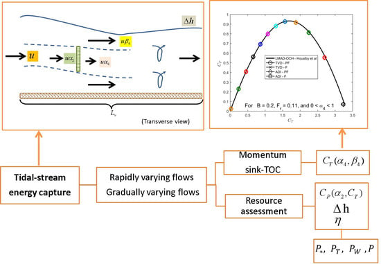
7]. To better represent the aquatic medium of tidal turbines analytical approaches introduced features of a finite flow; firstly by introducing a rigid lid surface and lately by considering a deformable surface and a turbine downstream region where turbine wake mixing occurs. This analytical model is known as the linear momentum actuator disc in open channel flow (LMAD-OCH) [
8]. Analysis of an actuator disc within a finite flow unveiled the importance of turbine bypass flow, blockage ratio (
B), and the turbine downstream mixing region; where
B indicates the fraction of a channel cross-sectional area occupied by the turbine.
A large number of potential regions for tidal power extraction are located in coastal areas; in these regions the use of finite flow is more appropriated as tidal streams are strongly influenced by the seabed and free-surface conditions. The consideration of these boundaries is relevant because they can significantly increase the amount of power extracted from the flow [
9,
10,
11]. This is because in shallow waters the seabed and free surface constraint effect in the turbine is more significant and produces a stronger blockage effect, which in turn increases the maximum power extractable by the turbine. On the other hand, a recent methodology, which undertakes natural boundaries in the power extraction analysis, uses a rather expensive computational technique and constrains the head drop produced by power extraction. This methodology uses a rapidly varying flow solver and shock fitting techniques to implement a line sink of momentum [
11,
12]. The line sink of momentum is based on the LMAD-OCH analytical model, which enable to determine a relation between upstream and downstream depth-average flow velocities and depths as a function of the turbine operating conditions. This relation is given by the relative change of head drop across the turbine. Line sink of momentum approach uses an RVF solver to compute the rapid changes produced by the tidal turbine power extraction in the water depth and flow velocities. The authors of [
11,
12] used a Godunov-type scheme, which implements a shock-fitting technique. The momentum extracted by turbines is simulated by computing the modification of mass and energy fluxes across the line sink of momentum. The region occupied by a turbine array acts as an interface between upstream and downstream conditions of the flow. This interface represents the elevation and velocity discontinuities produced by power extraction. Computation of the discontinuity which initially separates upstream and downstream conditions is equivalent to solving a Riemann problem [
13]; consequently, the Riemann solution indicates the flux through the discontinuity and therefore the shock propagation. To complete the line sink of momentum numerical representation, a condition on the head drop across the array is required [
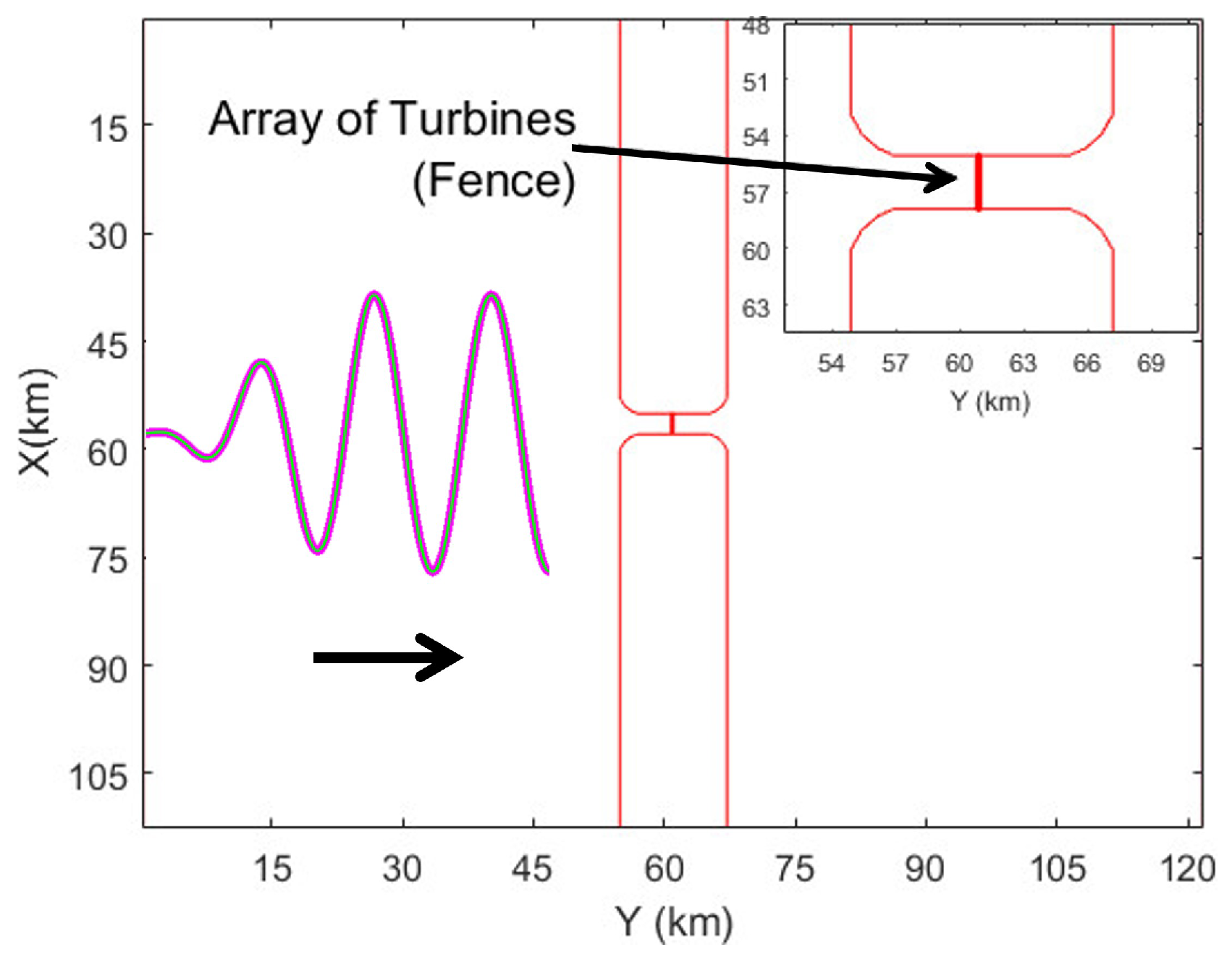
14]. This condition is given by the relative change of the head drop provided by the LMAD-OCH. This method was used to assess the tidal-stream potential of turbines configured as a fence in an idealised channel [
11]. Such a configuration was used in the Pentland Firth to estimate maximum power extracted, 4.2 GW, and the extractable power at the sub-channels [
15]. It was found that power availability varies according to the device operating conditions within the fences. A further refinement of the Pentland Firth estimation is given by [
16]; they reported a more conservative upper limit of 1.9 GW based on a large, but a viable blockage ratio (
0.4). Contrary to the line sink of momentum approach, in this research the momentum extracted by the turbines was simulated considering the turbine operating conditions and implementing a method that does not constrain the water elevation change. For this task the momentum sink TOC was used [
17], the method is based in LMADT-OCH and computes the axial component of the thrust force exerted by turbines to the flow by solving a sink term in the momentum equations. Consequently, momentum sink TOC incorporates the natural constraints of the coastal tidal-stream, the operating conditions of the turbine, and does not condition the head drop produced by power extraction. In this research, the momentum sink TOC was incorporated in a (1) conventional and (2) an innovative numerical solver to assess the resource. The conventional scheme solves gradually varying flows, which do not experience strong spatial gradients and are characterised by small Froude numbers. On the other hand, the innovative scheme solves rapidly varying flows that enable the simulation of flows, which experience discontinuities such as hydraulic jumps, flood waves, and shock waves. Therefore, a GVF solver simulates a flow that experiences smoother and slower changes than RVF. The rapidly varying flows solver implemented in this research is a shock-capturing model that consists of the algebraic combination of first-order and second-order upwind schemes. In this way, the model uses a low-order scheme to simulate the regions where strong gradients exist and spurious numerical solutions are likely to appear. This solver constitutes an efficient approach for simulating energy capture in rapidly varying flows because the scheme is not required to solve the Riemann problem at each grid, where an array of turbines are defined, to compute the discontinuities produced in the flow due to power removal. Solving the Riemann problem represents an expensive procedure in computational terms [
18]
Two turbine configurations were selected to assess the resource at a regional scale: A fence and a partial fence. Partial-fence configuration covers a selected part of a channel cross-section producing flow diversion. Part of the stream passes through the array, experiencing velocity reduction due to the momentum loss, and the rest bypass the array, presenting velocity intensification when circumventing the partial fence. This scenario is referred to as unbounded flow and two analytical theories describe power extraction with this type of flow: (i) The LMAD-OCH and (ii) two scales models, their main characteristics are described below. LMAD-OCH studies a partial fence as a long row [
11], and in this way, upstream conditions can be assumed to be uniform, and marine turbines within the array can be represented by actuator discs. This approach estimates the momentum extracted by a partial fence and provides information on energy lost only within the turbine’s near field region (
) [
11], i.e., just downstream of the turbine. LMAD-OCH is also referred to as a single-scale model [
19] because the quasi-inviscid flow assumption used in the theory allows important turbulent mixing to occur at a far downstream region (
) where the pressure equilibrates across the channel cross-section. The
region is smaller than the far downstream region (
). Within the
region the quasi-inviscid assumption of LMAD-OCH enables the estimation of turbine-scale wake mixing, which occurs just downstream of the turbine and it is not significant in comparison to the array-scale wake mixing. This quasi-inviscid model is consistent with three-dimensional actuator disc computations of mixing just downstream of the turbines [
20]. Therefore, the LMAD-OCH theory enables the parametrisation of turbine-wake mixing within the near-field region, in this region it is assumed that elevation and velocity perturbations due to power extraction occur. This assumption captures vertical flow variations produced by horizontal mixing effects at the turbine scale [
21]. In contrast to the LMAD-OCH theory, the two scale model studies energy extraction via a partial fence considering two scales of flow: (a) A turbine scale flow, which describes the flow around a single turbine and the wake of the turbine, studied by [
8] and (b) a array scale, which is the large-scale flow around the turbine array and the array wake [
22]. The two scales’ separation implies that the flow bypassing the turbine occurs faster than the horizontal expansion of the flow bypassing the entire array, and analyses power extraction as two quasi-inviscid open channel flow problems. The two scales are linked via the upstream boundary condition of the turbine-scale flow because power extraction produces a flow diversion around the array and reduces the mass flux through the array and this mass flux reduction provides the upstream boundary to the turbine scale [
23]. Initially, a single long turbine row and a rigid lid surface approximation which did not account for the effect of changes in water depth were considered [
22]. Later, a better accounting for the interaction of the device- and array-scale flow events enabled the analytical and numerical study of short rows [
20]. Recently, [
24] included a deformable free-surface in the two-scale analysis by incorporating finite Froude (
) numbers in the analysis and consequently accounting for a deformable surface.
Analytical models provide an understanding of the physics involved in tidal-stream power extraction; however, numerical simulations are required to provide a more complete analysis of the effects of tidal energy extraction. In this context, the two-dimensional approach, the line sink of momentum was developed to assess tidal-stream resource with a long partial fence, through the solution of shallow water equations. The method was used to numerically estimate the force applied by a porous disc in scale experiments [
25], and to identify the power available at an idealised coastal headland [
26] and at Anglesey Skerries, off the Welsh coast [
12]. On the other hand, attempts to numerically couple the turbine scale with the array scale are limited to three-dimensional simulations of small turbine arrays [
27], which require high-fidelity turbine scale simulations; this methodology has not been applied to regional scale [
21].
In this research, tidal-stream energy resource at regional scale was evaluated in two scenarios: bounded and unbounded flows, which were represented with a fence and a partial-fence turbine array configuration, respectively. The energy capture by the arrays was simulated with the momentum sink TOC method, which numerically implements the LMAD-OCH theory. To investigate the role of numerical solution schemes for simulating tidal energy capture, the momentum sink TOC was implemented in two hydrodynamic models that use a conventional (GVF) and up-to-date (RVF) solution scheme. The novelty of this research lays in the numerical representation of energy capture by arrays of turbines considering (i) a flow more representative of coastal regions, (ii) not conditioning of head drop across a turbine array, (iii) use of hydrodynamic models which are able to represent realistic coastal scenarios, and (iv) implementation of an efficient RVF solver that uses a shock-capturing scheme. The methodology proposed will enable the identification of a less computationally expensive numerical tool that provides a reliable evaluation of the resource in realistic scenarios.
3. Resource Assessment
Though a significant amount of power could be extracted if high blockage ratios were used, this procedure presents adverse effects such as (i) significant flow rate reduction [
40], (ii) tidal hydrodynamics affectation, and (iii) mixing and transport processes impact at turbine scale and regional scale [
6,
21,
41,
42]. As a result of this evidence, evaluation of tidal-stream resource is performed within realistic blockage ratios (
) as a post-processing stage.
Indicators used to assess the energy resource were the following metrics: Total power extracted, power dissipated by turbine wake mixing, and power available for electrical generation. The procedure used to calculate them follows. The initial step was the election of turbine operating conditions and calculation of turbine velocity coefficient (Equation (10)). Subsequently, thrust (Equation (7)) and power (Equation (12)) coefficients associated to the turbine were estimated. The next step was identification of head drops across the array and turbine efficiency (Equation (13)). These two parameters enable estimation of total power extracted (Equation (14)), power dissipated by turbine wake mixing (Equation (15)), and power available for electrical generation (Equations (11) and (16)).
The operating conditions of the turbine and the turbine configurations evaluated with ADI and TVD models are specified in the four scenarios reported in
Table 1.
3.1. Thrust and Power Coefficients Time Series
Calculation of
and
required specification of the wake induction factor, which depends on the location of the turbine within the array and the local tidal dynamics [
26] as both affect turbine wake mixing. However, to maximise power available for electrical generation the downstream core flow (
) was adjusted by setting the wake induction factor to
= 1/3 [
43,
44]. A constant
was used during the simulation; however, a slightly better power available is obtained if a variable wake induction factor is used [
12].
Thrust and power coefficients are functions of the upstream conditions through the Froude number used in
calculation; therefore,
and
are modulated by the tidal cycle. Thrust and power coefficients time series were obtained from both models using a fence configuration constituted by turbines with a relatively large blockage ratio (
). The time series from an
tidal cycle and taken from the middle of the channel, where the array was deployed, are shown in
Figure 3a,b.
and
time series present two maximum values that correspond to maximum flood tide and maximum ebb tide velocities. Comparison between the solutions obtained from the models indicate that ADI produces slightly higher magnitudes of
(
) and
(
) than TVD’s
and
. Time-average of
and
obtained from ADI and TVD are consistent with LMADT-OCH analytical model and they indicate upper limits for these coefficients.
Additionally, time series obtained with ADI present a phase delay evident in the maximum values. ADI’s phase delay was evident at stream-wise velocity component of tidal current at natural state. This behaviour was consistent along the domain, i.e., it was not restricted to the channel, suggesting that the delay may be related to the different solution scheme employed by the models. However, further understanding of phase simulated by both models would require examination of field observations of free surface elevation and depth-averaged flow velocity. It is worth noticing that the parameters to be presented in the following sections refer to values averaged over a tidal period; therefore, the phase delay reported by ADI time series does not influence the results presented.
The larger magnitude of
reported by ADI is associated with the smaller affectation of the momentum extraction on the bypass velocity reduction (represented by
). ADI underestimation of velocity reduction due to power extraction was reported by [
45]. In the case of
, the turbine velocity coefficient reduces the difference between the magnitudes obtained from the models.
3.2. Upstream Velocities
Contrary to a tidal fence configuration, where energy extraction produce uniform conditions along the array and a middle-fence cell capture this dynamic, the implementation of a partial fence produces a scenario where energy extraction occurs along a limited section of the cross-channel, indicating the existence of array-bypass flows. To identify the effects of a partial fence on the upstream velocities, the time-averaged stream-wise component of velocity was calculated at each grid cell that constitutes the partial fence. Upstream velocities normalised by natural state velocities and obtained for increasing values of blockage ratio computed with ADI and TVD are presented in
Figure 4. Upstream velocities along the fence tend to be uniform for small blockage ratios (
), but further increase of
B influence differently the grid-cells located at the middle and at the edges of the partial fence. Large values of
B produce higher velocity decreases in the middle of the array, meanwhile the edges exhibit smaller velocity reduction. A comparison of results obtained from both models shows that upstream velocities from ADI present smaller reductions with increasing
B than TVD. In addition, for small
B, velocities at the edges of the partial fence simulated with ADI show a slight magnitude enhance. This suggests that the faster array-bypass flow computed with ADI model is influencing the velocities at the partial-fence edges. The smaller velocity reduction presented in ADI’s velocity solutions is consistent with [
45]. They indicated that a gradual varying flow scheme under-estimate the velocity decrease produced by momentum extraction; meanwhile, a rapidly varying flow scheme approximates more accurately this reduction due to its capacity to solve the velocity spatial gradients generated during energy extraction.
3.3. Head Drop and Turbine Efficiency
Estimation of turbine efficiency required calculation of head drop across the array.
was calculated using an analytical and numerical approach. Analytical solutions were obtained by solving a cubic polynomial, which represents a condition on the head drop across the array obtained from LMADT-OCH [
8]. Coefficients of the polynomial are a function of blockage ratio, thrust coefficient, and Froude number.
and
were obtained from TVD simulations, as this scheme approximates the velocity reduction more accurately for a fence scenario [
45]. Meanwhile, numerical solutions correspond to head drops obtained from depth differences across the array at upstream and downstream locations. These locations correspond to the neighbouring upstream and downstream cell. In the case of a 16 m diameter device, the mean axial upstream velocities are recovered to about 80% [
46,
47] within 160 m; therefore, the grid size used in this research (
= 150 m) is of the order of the turbine wake length suggesting that the neighbouring cell approximates the upstream conditions of the flow. Maximum head drops within a tidal cycle were calculated for increasing
B,
obtained analytically and numerically using a fence (
Figure 5a) and a partial fence (
Figure 5b) were compared. For bounded-flows, analytical and numerical solutions are similar; however, a GVF scheme (
Figure 5a.1) produces a solution more consistent with the analytical solution (
Figure 5a). In the case of unbounded flows, the analytical solution of LMAD-OCH indicates a homogeneous water drop along the partial fence for given blockage ratio (
Figure 5b). This solution is consistent with the 1D assumption of the theoretical model [
9,
43]. Conversely, numerical solutions indicate non-uniform head drops along the array for increasing
B values. Within the partial fence, maximum values of head drop are found in the middle cells, while smaller depth change are exhibited towards the edge of the array. Comparison of
obtained from TVD and ADI models for a partial fence indicate that TVD simulates larger head drops (
Figure 5b.2). Additionally, for small
B,
at the middle-cells of the array obtained from TVD are similar to analytical solutions; however, for
, the head drop magnitudes become smaller than the analytical solution. These results indicate that rapidly varying flow solver provides a reasonable insight into the effect of small blockage ratios on the head drop across the partial fence, where
is influenced by the bypass flow producing a head drop reduction at the edges of the partial fence.
Turbine efficiencies were estimated for increasing blockage ratios. Analytical and numerical solutions of
for flows characterised by small Froude numbers were calculated, as the solutions were found to be consistent only numerical solutions are reported. These solutions are functions of the head drops obtained with ADI and TVD. Time-averaged and array-averaged turbine efficiencies calculated for both configurations: fence and partial fence are presented in
Figure 6a,b, respectively. Turbine efficiencies were plotted against the time-averaged, array-averaged thrust coefficients. Increasing
B values indicate a gradual efficiency reduction but thrust coefficient augmentation. Maximum turbine efficiency found (
) correspond to the smaller blockage ratio tested (
0.05) and this value is associated to
1.0; meanwhile, blockage ratio increases to
0.4 produce a turbine-efficiency reduction (
) and thrust coefficient increase (
3.5). Efficiency decrease with
B augmentation is explained by the larger energy dissipated due to turbine-wake mixing [
48]. On the other hand, the analytical study of further blockage ratio increase (
) indicates a slow turbine-efficiency decrease rate [
14]. This trend indicates that for a very large
B, subsequent dimension augmentation produces a small efficiency reduction; such a scenario is attractive; however, large blockage ratios are not a practical option.
Comparison of ADI and TVD solutions from a partial fence shows similar results; however, slightly higher efficiency values are reported with TVD. As the efficiency is a function of
, higher
’s are explained by the larger head drops obtained with RVF scheme. Furthermore, comparison of the solutions obtained from both configurations indicate a high degree of similarity. This consistency suggest that the partial fence is long enough to resemble conditions similar to a fence at the turbine’s near-field region. It is worth mentioning that turbine efficiencies calculated for a partial fence do not capture the power dissipated by the array-wake mixing, because LMAD-OCH theory only describes the energy extraction dynamic within the turbine’s near-field region [
20,
23]. In this region, wake mixing produced by individual turbines occurs and flow’s uniform conditions are recovered; therefore, wake mixing generated by the array is not included in the analysis.
3.4. Power Metrics
To compare the performance of a partial fence with a fence, time-averaged and array-averaged power metrics were obtained from both configurations. Total power extracted estimated with ADI and TVD are presented in
Figure 7(a.1,a.2), respectively.
is a function of water drop and the increase of blockage ratio produces a head drop augmentation which is responsible of larger values of total power extracted. For bounded flows (F), [
45] indicated that
is accurately approximated by an ADI model because a GVF solver approximates better the head drops across a fence. For unbounded flows scenario (PF),
magnitudes obtained from ADI and TVD are smaller than the fence. This result is explained by the head drop reported by the models for the partial fence; smaller
magnitudes were obtained for this configuration due to the reduced head drops at the edges of the array. The comparison of
obtained by the models for the partial fence indicate that TVD scheme produces larger magnitudes of total power extracted. These solutions are more reliable as TVD approximates better the head drop across a partial fence. The power dissipated by turbine-wake mixing estimated with both ADI and TVD models are shown in
Figure 7(b.1,b.2), respectively.
depends on the turbine efficiency and the total power extracted, which in turn is strongly influenced by the head drop across the turbine array. This dependency indicates that
solutions are also explained by head drop values. For bounded flows,
values obtained with ADI are reliable solutions [
45]. In the case of unbounded flows scenario,
magnitudes obtained from the models are slightly smaller than the fence. This result is expected as smaller
were obtained for the partial fence. The comparison of
obtained from the models for the partial fence, indicate that TVD produces larger magnitudes of power lost. TVD solutions are more accurate due to the better approximation of the head drop for unbounded flows provided by the model.
Regarding the power removed by the turbine, two metrics were calculated. First, in function of turbine efficiency and second, in terms of cubic velocity P. These metrics are expected to be consistent as they describe the amount of power available for electricity generation.
Power available in terms of turbine efficiency estimated with ADI and TVD are presented in
Figure 8(a.1,a.2), respectively.
is a function of total power extracted and consequently depend on the head drop. For bounded flows,
is better approximated by an ADI scheme; however, for unbounded flows scenario, this metric is better simulated by an TVD scheme.
On the other hand, power available in terms of cubic velocity calculated with ADI and TVD are presented in
Figure 8(b.1,b.2), respectively.
P magnitude depends on the upstream velocity and for bounded flows, [
45] reported the incapacity of ADI model to satisfactorily approximate the velocity reduction due to power extraction. This underestimation of velocity decrease for increasing values of blockage ratio explains the large values of
P reported by ADI for both configurations. Meanwhile,
P obtained with TVD for a fence and a partial-fence configuration present magnitudes similar to
obtained from both ADI and TVD models. This result indicates that TVD scheme better approximates the consistency between
P and
for both configurations. ADI fails to represent this consistency as ADI underestimate the velocity reduction due to power extraction and consequently report higher values of Power than TVD. On the other hand, TVD simulates better this velocity reduction, so powers in function of velocity are better solved by TVD and these values are more consistent with the power in function of turbine efficiency.
4. Discussion and Conclusions
This research implemented momentum sink TOC method in two hydrodynamic models that can solve realistic coastal scenarios to simulate marine turbine configurations and to perform tidal-stream resource assessment. Contrary to the conventional consideration of constant thrust coefficient [
4,
6,
49], the use of turbine operating conditions to calculate the thrust force, imparted by the turbine on the stream, enabled the calculation of non-constant thrust and power coefficients. These coefficients undertake the tidal regime specific to a potential site and allow the use of tailored values of
and
to assess the resource, therefore providing a more realistic numerical representation of the turbine.
In contrast to [
11], the head drop across the array used to assess the resource was obtained from the depth difference between the array upstream and downstream location. The use of a no-fixed head drop in a partial fence enabled the identification of non-uniform conditions along the array. This configuration represented the simulation of an unbounded flow, which favours the existence of two regions: array-bypass flow and array-wake flow. These regions describe the velocity intensification when bypassing the array, and the significant velocity diminution downstream of the array due to array-wake mixing. Flow conditions along the partial fence are not uniform as array-bypass flows influence the upstream velocity and water depth at the edges of the array. These features illustrates the effect of a partial fence on the free flow as reported by [
23,
50] and indicate the advantage of using numerical tools to evaluate the tidal-stream resource and complement analytic models.
In terms of turbine efficiency, both turbine configurations showed consistent efficiencies. The similarity of the results could be explained by the use of the same wake-induction factor (
), which is used for the turbine velocity coefficient (
) calculation [
45]. The turbine efficiency used in this research considers the turbine-wake mixing within the near-field region. Over the near-field length scale, it is assumed that flow passing through the fence and partial fence mixes and leads to a smooth vertical profile similar to upstream profiles [
43]. This assumption captures vertical flow variations produced by horizontal mixing effects at the turbine scale [
21]. The models compute the turbulence generated by turbine-wake mixing correctly by implementing (i) turbulence induced by the bottom friction and (ii) inviscid flow assumption [
51].
This research assesses upper limits for tidal-stream resource assessment in a semi-narrow tidal channel using the
tidal constituent. Additionally, evaluation of two turbine configurations allowed the identification of the numerical scheme that performs more accurate tidal-stream energy resource evaluation. Opposite to conventional methodologies to assess the resource, where tidal energy extracted by marine turbines was approximated with a bottom roughness [
40,
52,
53] and a momentum sink [
6,
47,
49,
54], the numerical implementation of LMADT-OCH enabled the calculation of the turbine efficiency. This parameter provided a distinction between total power extracted, power available for electrical energy generation, and power dissipated by turbine-wake mixing. Evaluation of the conventional scheme to assess tidal-stream (ADI model which solves GVF) and a scheme with shock-capturing capability (TVD model which solves RVF), indicate that unbounded flow scenarios are better assessed with a TVD scheme. The better approximation of the head drops and velocities reduction by a TVD model for a partial-fence scenario implies that a rapidly varying flow solver is required to calculate an upper bound for tidal-energy extraction when a realistic configurations of turbines is used. The conclusions of this work are as follows:
Depth perturbations due to power extraction were solved by both models ADI and TVD. A satisfactory head drop was approximated with TVD scheme for both turbine configurations, indicating that water depth gradients are better solved by the shock-capturing capability.
The total power extracted (), available power in terms of the turbine efficiency (), and power dissipated by turbine-wake mixing (), were correctly calculated by the models. For a tidal fence, power metrics were better computed by the scheme that solves slow and smooth flows, because the head drop across the array simulated by this scheme was more accurate. In the case of a partial fence, the power metrics were better approximated by solving a rapidly varying flow solution.
Simulation of unbounded flows scenario with sink TOC method and RVF solver indicates non-uniform conditions along the partial fence, contrary to one-dimensional LMAD-OCH.
In terms of power removed by turbines as a function of the upstream velocity (P), this metric is better solved by an RVF solver as this model correctly represents the flow velocity reduction produced by power extraction.


