Single-Layer Transmitter Array Coil Pattern Evaluation toward a Uniform Vertical Magnetic Field Distribution


Abstract
1. Introduction
2. Materials and Methods
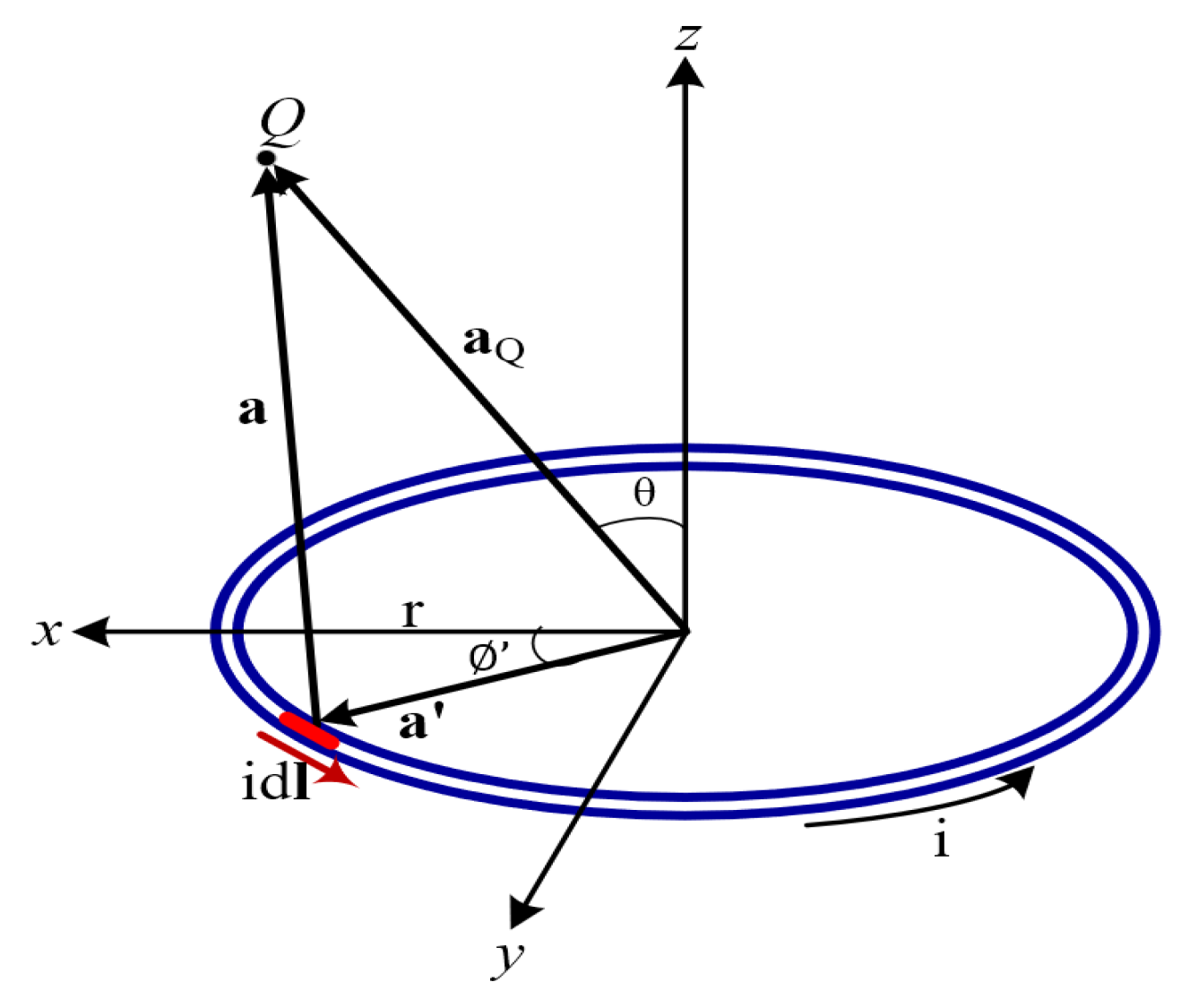
2.1. Biot-Savart Law
2.2. The Off-Symmetrical Axis Magnetic Field Formulation due to a Circular Current Loop
2.3. Analysis and Evaluation Method
- (1)
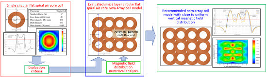
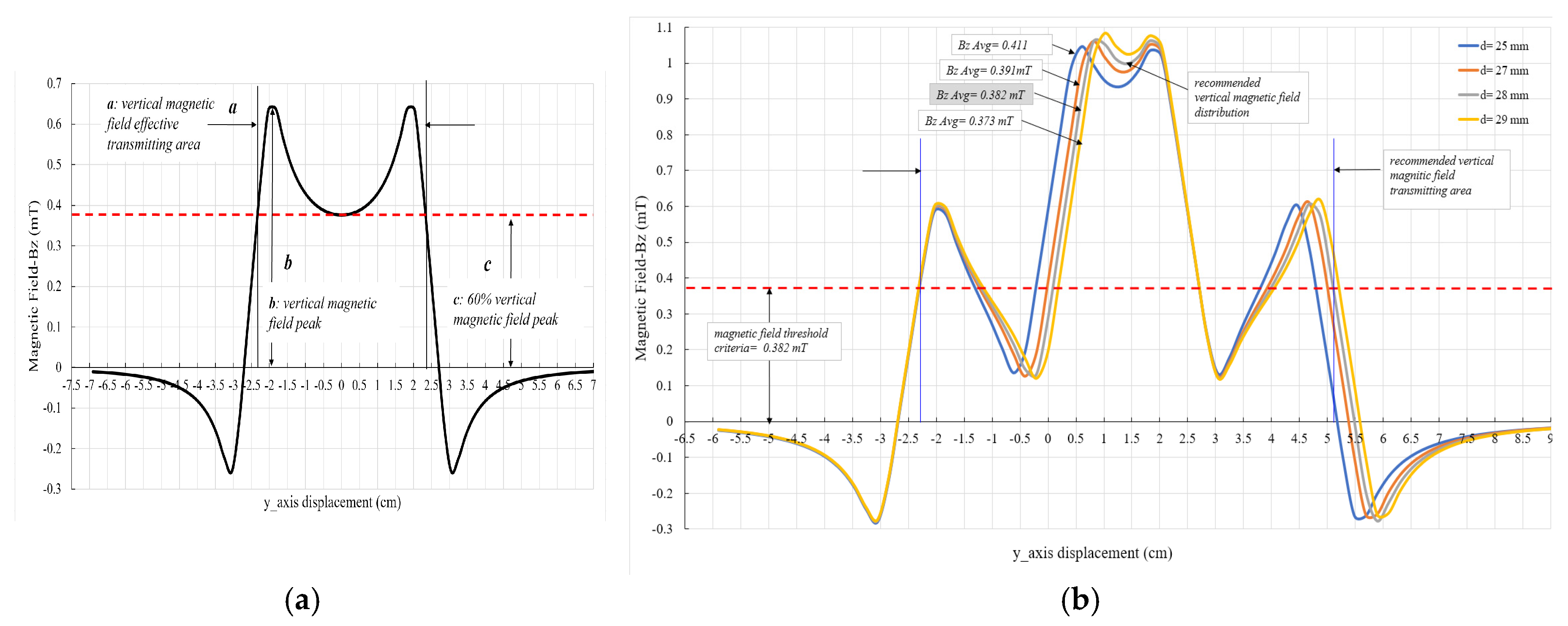
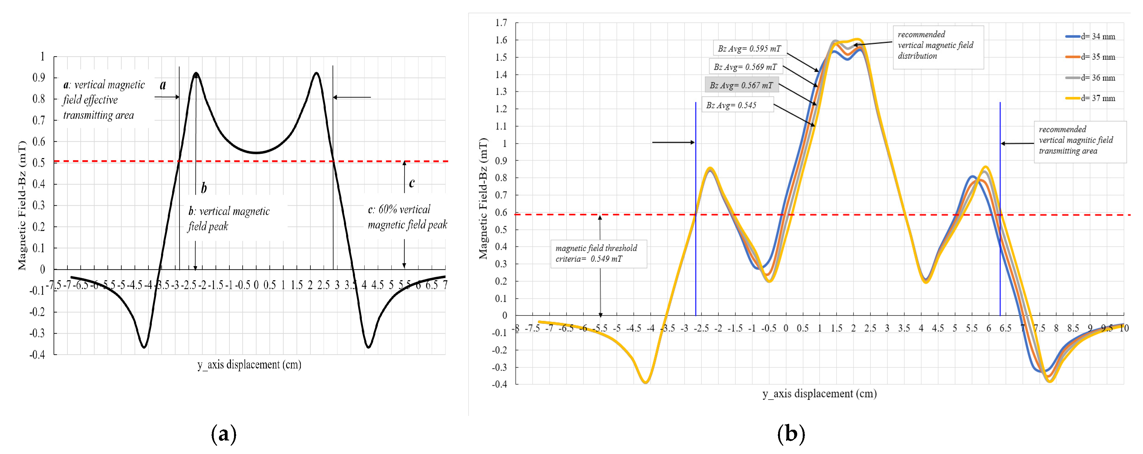
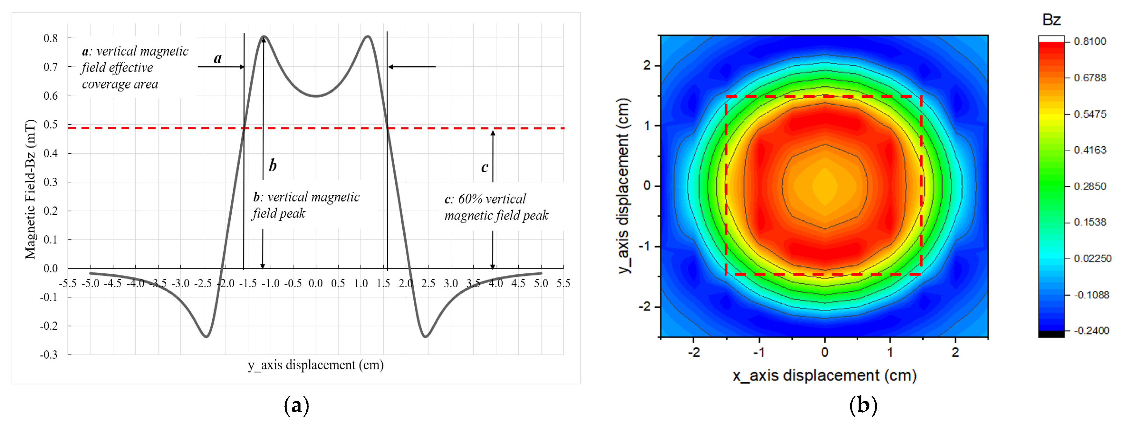
- In the first scenario, the vertical magnetic field distribution of single coil model with different coil parameter is analysed and evaluated. The vertical magnetic field distribution characteristic of single coil evaluation result is used to define the evaluation criteria for analyses and evaluation of the array coil models vertical magnetic field distribution. The vertical direction evaluation distance is defined at 2.5 mm from the coil surface with a unit current at 1 Ampere. The array coil model vertical magnetic field distribution is analyzed and evaluated with a variation in distances between the adjoining coil centers to meet the vertical magnetic field uniform distribution with the transmitting area as wide as possible. The evaluation criteria used in this paper is proposed as follows:
- (a)
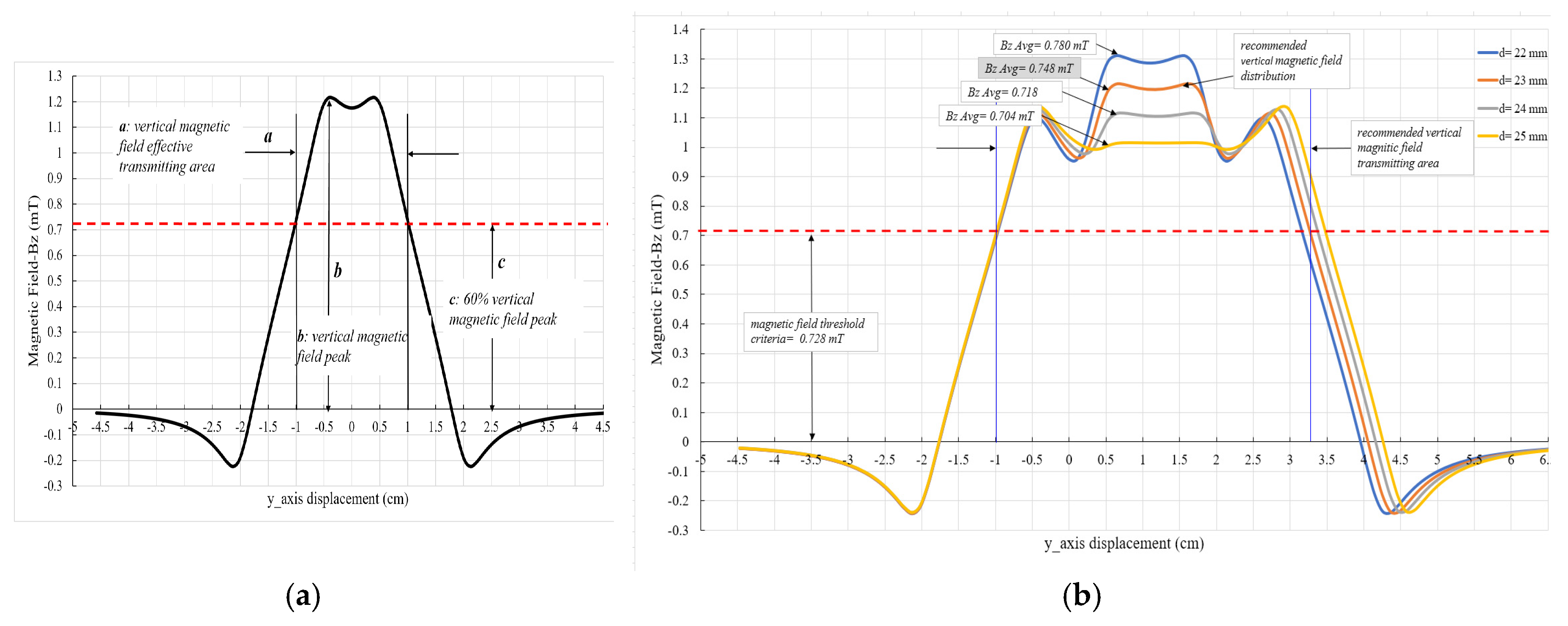
- Average vertical magnetic field resultant is not less than 60% single coil vertical magnetic field peak, and
- (b)
- Magnetic field effective transmitting area is as wide as possible.
- (2)
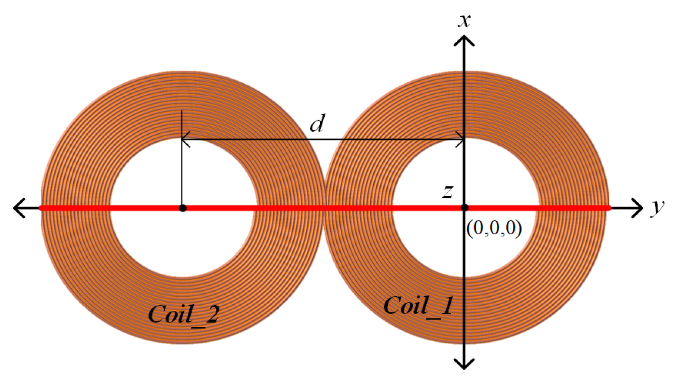
- The second scenario is a case study. The general investigation result from the first evaluation scenario is applied in the array coil model design. In this evaluation scenario, different array coil model patterns which are composed of 2, 3, 4, and 6 coils are constructed from identical circular flat spiral air-core coils with given coil parameters. The vertical magnetic field distribution is analyzed and evaluated using the proposed method as described in first evaluation scenario with variety in the distance between the adjoining coil centers. The goal evaluation in this case study is recommended array coil model with close to uniform vertical magnetic field distribution and widely effective transmitting area. The array coil model patterns are shown in Figure 5.
3. Numerical Evaluation of the Vertical Magnetic Field Distribution
3.1. The Coil with Different Coil Parameter
3.2. Discussion
4. Case Study
4.1. Single Coil Evaluation
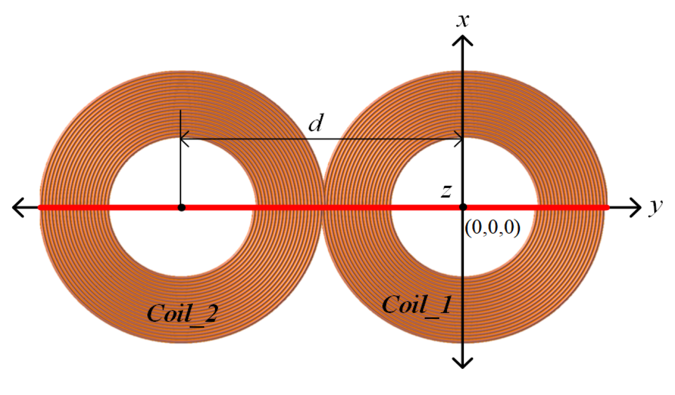
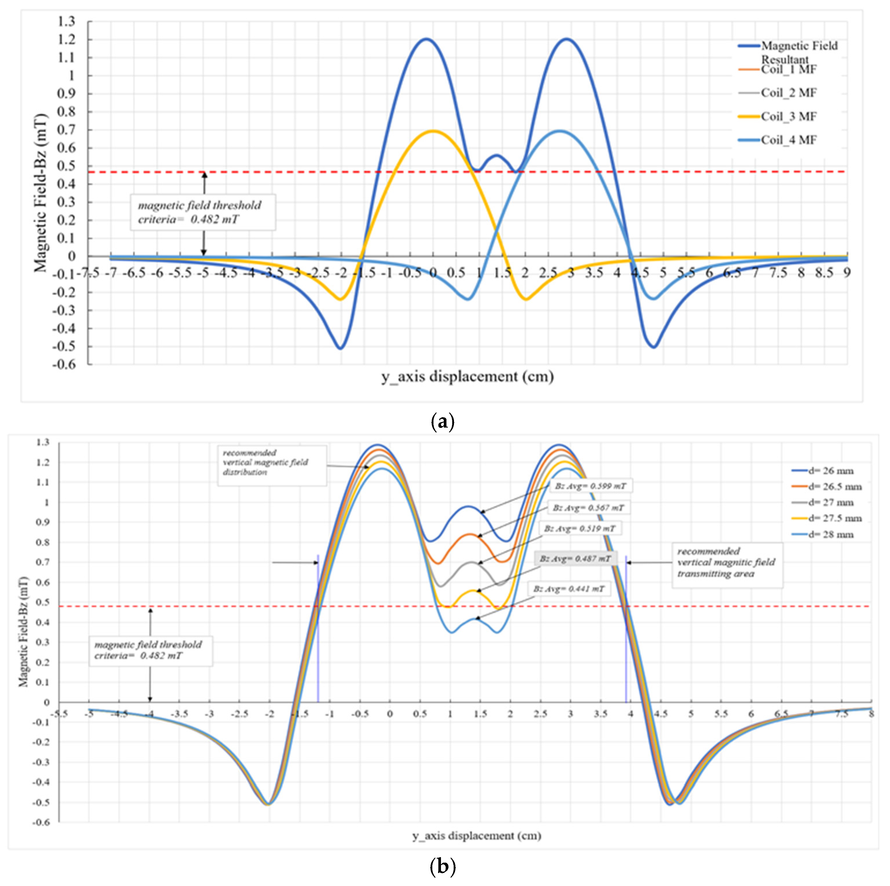
4.2. The Two Coils Pattern Evaluation
4.3. The Three Coils Pattern Evaluation
4.4. The Four Coils Pattern
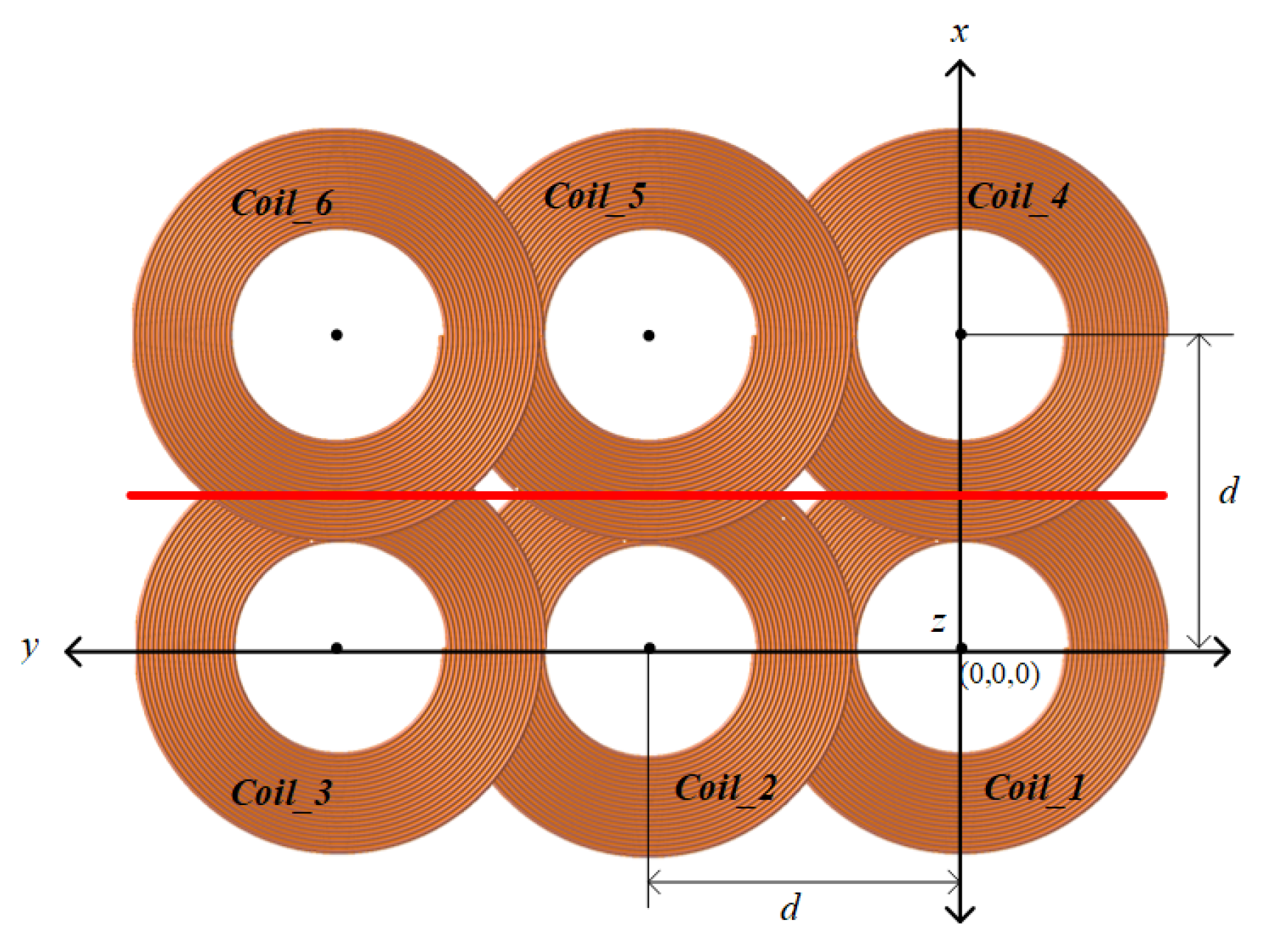
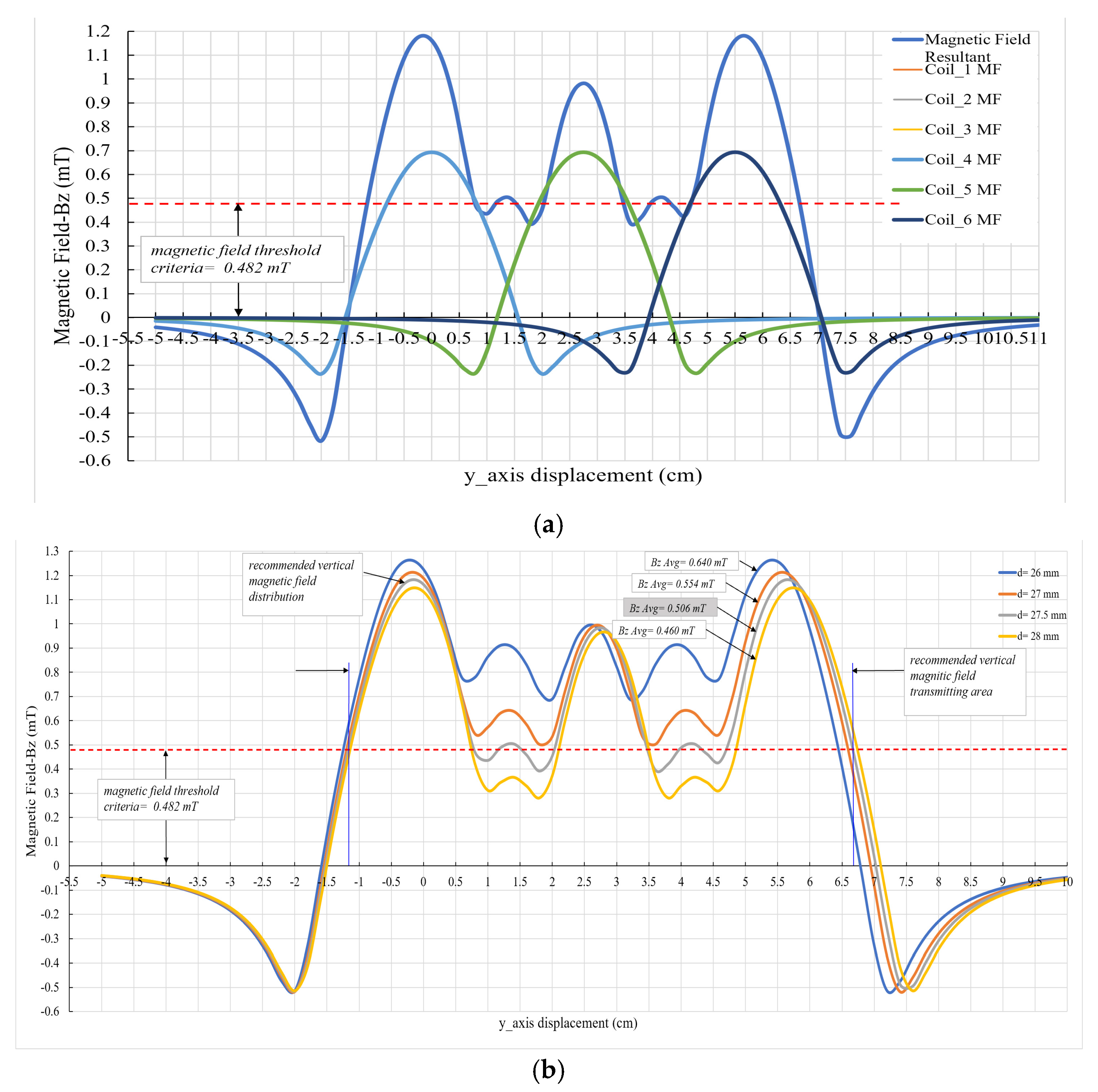
4.5. The Six Coils Pattern
4.6. Discussion
5. Conclusions
Author Contributions
Funding
Acknowledgments
Conflicts of Interest
References
- Jang, Y.; Jovanovic, M.M. A contactless electrical energy transmission system for portable-telephone battery chargers. IEEE Trans. Ind. Electron. 2003, 50, 520–527. [Google Scholar] [CrossRef]
- Kim, C.; Seo, D.; You, J.; Park, J.; Cho, B. Design of a contactless battery charger for cellular phone. IEEE Trans. Ind. Electron. 2001, 48, 1238–1247. [Google Scholar]
- Choi, B.; Nho, J.; Cha, H.; Ahn, T.; Choi, S. Design and implementation of low-profile contactless battery charger using planar printed circuit board windings as energy transfer device. IEEE Trans. Ind. Electron. 2004, 51, 140–147. [Google Scholar] [CrossRef]
- Hui, S.Y.R.; Ho, W.W.C. A new generation of universal contactless battery charging platform for portable consumer electronic equipment. IEEE Trans. Power Electron. 2005, 20, 620–627. [Google Scholar] [CrossRef]
- Sakamoto, H.; Harada, K.; Washimiya, S.; Takehara, K. Large air-gap coupler for inductive charger. IEEE Trans. Magn. 1999, 35, 3526–3528. [Google Scholar] [CrossRef]
- Joung, G.B.; Cho, B.H. An energy transmission system for an artificial heart using leakage inductance compensation of transcutaneous transformer. IEEE Trans. Power Electron. 1998, 13, 1013–1022. [Google Scholar]
- Neugebauer, T.C.; Perreault, D.J. Filters with inductance cancellation using printed circuit board transformers. IEEE Trans. Power Electron. 2004, 19, 591–602. [Google Scholar] [CrossRef]
- Shiri, A.; Moghadam, D.E.; Pahlavani, M.R.A.; Shoulaie, A. Finite element-based analysis of magnetic forces between planar spiral coils. J. Electromagn. Anal. Appl. 2010, 2, 311–317. [Google Scholar] [CrossRef]
- Andris, P.; Weis, J.; Frollo, I. Magnetic field of spiral-shaped coil. In Proceedings of the 7th International Conference on Measurement, Bratislava, Institute of Measurement Science SAS, Smolenice, Slovakia, 20–23 May 2009; pp. 262–265. [Google Scholar]
- Singh, V.; Qusba, A.; Roy, A.; Castro, R.A.; McClure, K.; Dai, R.; Greenberg, R.J.; Weiland, J.D.; Humayun, M.S.; Lazzi, G. Specific absorption rate and current densities in the human eye and head induced by the telemetry link of an epiretinal prosthesis. IEEE Trans. Antennas Propag. 2009, 57, 3110–3118. [Google Scholar] [CrossRef]
- Waffenschmidt, E. Homogeneous magnetic coupling for free positioning in an inductive wireless power system. Emerging and Selected Topics in Power Electronics. IEEE J. Emerg. Sel. Top. Power Electron. 2015, 3, 226–233. [Google Scholar] [CrossRef]
- Minnaert, B.; Stevens, N. An improved algorithm for the creation of homogeneous magnetic field distributions. In Proceedings of the 2015 International Conference on Electromagnetics in Advanced Applications (ICEAA), Turin, Italy, 7–11 September 2015; pp. 517–520. [Google Scholar]
- Azpúra, M.A. A semi-analytical method for the design of coil-systems for homogeneous magnetostatic field generation. Prog. Electromagn. Res. B 2012, 37, 171–189. [Google Scholar] [CrossRef]
- Minnaert, B.; Strycker, L.D.; Stevens, N. Design of a Planar, Concentric Coil for the Generation of a Homogeneous Vertical Magnetic Field Distribution. ACES J. 2017, 32, 1056–1063. [Google Scholar]
- Nguyen, M.Q.; Hughes, Z.; Woods, P.; Seo, Y.-S.; Rao, S.; Chiao, J.-C. Field Distribution Models of Spiral Coil for Misalignment Analysis in Wireless Power Transfer Systems. IEEE Trans. Microw. Theory Tech. 2014, 62, 920–930. [Google Scholar] [CrossRef]
- Cortes, I.; Kim, W.-J. Lateral Position Error Reduction Using Misalignment-Sensing Coils in Inductive Power Transfer Systems. IEEE/ASME Trans. Mechatron. 2018, 23, 875–882. [Google Scholar] [CrossRef]
- Liu, X.; Hui, S.Y.R. Simulation Study and Experimental Verification of a Universal Contactless Battery Charging Platform with Localized Charging Features. IEEE Trans. Power Electron. 2007, 22, 2202–2210. [Google Scholar]
- Hayt, W.H.; Buck, J.A. Engineering Electromagnetics, 8th ed.; The McGraw-Hill Companies, Inc.: New York, NY, USA, 2012; ISBN 978-0-07-338066-7. [Google Scholar]
- Smythe, W.R. Static and Dynamic Electricity, 2nd ed.; McGraw-Hill: New York, NY, USA, 1988; pp. 270–271. [Google Scholar]
- Simpson, J.; Lane, J.; Immer, C.; Youngquist, R. Simple Analytic Expressions for the Magnetic Field of a Circular Current Loop. NASA Technical Reports Server. Available online: https://ntrs.nasa.gov/archive/nasa/casi.ntrs.nasa.gov/20010038494.pdf (accessed on 17 October 2019).


| Parameter | Coil_1.1 | Coil_1.2 |
|---|---|---|
| Number of turns (N) | 23 | 8 |
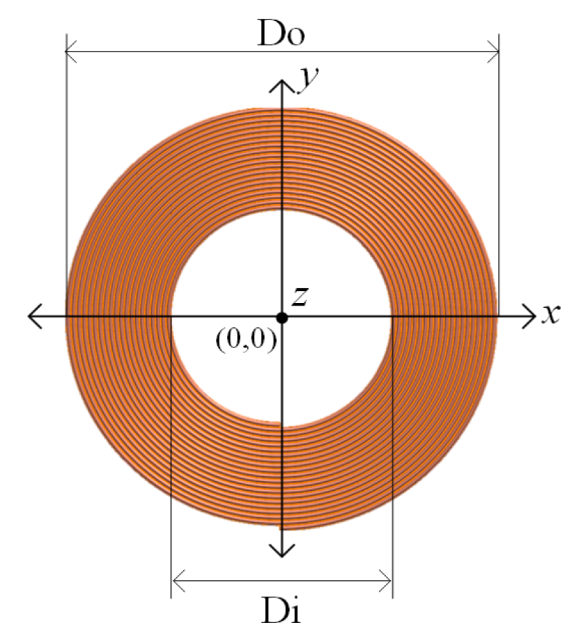
| Inner diameter (Di) (mm) | 10 | 30 |
| Outer diameter (Do) (mm) | 40 | 40 |
| Pitch (P) (mm) | 0.03 | 0.03 |
| Wire diameter (W) (mm) | 0.643 | 0.643 |
| Parameter | Coil_2.1 | Coil_2.2 |
|---|---|---|
| Number of turns (N) | 37 | 15 |
| Inner diameter (Di) (mm) | 20 | 40 |
| Outer diameter (Do) (mm) | 60 | 60 |
| Pitch (P) (mm) | 0.03 | 0.03 |
| Wire diameter (W) (mm) | 0.643 | 0.643 |
| Parameter | Coil_3.1 | Coil_3.2 |
|---|---|---|
| Number of turns (N) | 38 | 23 |
| Inner diameter (Di) (mm) | 30 | 45 |
| Outer diameter (Do) (mm) | 80 | 80 |
| Pitch (P) (mm) | 0.03 | 0.03 |
| Wire diameter (W) (mm) | 0.643 | 0.643 |
| Coil Parameters | 60%Bz-Peak/Bz Avg (mT) | The Width of Transmitting Area (mm) | The Distance between the Adjoining Coil Center (mm) | ||
|---|---|---|---|---|---|
| Single Coil | 1 × 2 Array Coil | Single Coil | 1 × 2 Array Coil | 1 × 2 Array Coil | |
| Di = 10 mm, Do = 40 mm, N = 23 | 0.728 | 0.748 | 20 | 50 | 23 |
| Di = 30 mm, Do = 40 mm, N= 8 | 0.244 | 0.248 | 35 | 55 | 22 |
| Di= 20 mm, Do = 60 mm, N= 37 | 0.803 | 0.805 | 35 | 72 | 38 |
| Di = 40 mm, Do = 60 mm, N= 15 | 0.382 | 0.382 | 45 | 75 | 28 |
| Di = 30 mm, Do = 80 mm, N = 38 | 0.733 | 0.733 | 45 | 85 | 42 |
| Di = 45 mm, Do = 80 mm, N = 23 | 0.549 | 0.567 | 50 | 90 | 36 |
| Parameter | Single Coil |
|---|---|
| Number of turns (N) | 17 |
| Inner diameter (Di) (mm) | 25 |
| Outer diameter (Do) (mm) | 47.8 |
| Pitch (P) (mm) | 0.03 |
| Wire diameter (W) (mm) | 0.643 |
© 2019 by the authors. Licensee MDPI, Basel, Switzerland. This article is an open access article distributed under the terms and conditions of the Creative Commons Attribution (CC BY) license (http://creativecommons.org/licenses/by/4.0/).
Share and Cite
Luo, W.-J.; Kuncoro, C.B.D.; Pratikto; Kuan, Y.-D. Single-Layer Transmitter Array Coil Pattern Evaluation toward a Uniform Vertical Magnetic Field Distribution. Energies 2019, 12, 4157. https://doi.org/10.3390/en12214157
Luo W-J, Kuncoro CBD, Pratikto, Kuan Y-D. Single-Layer Transmitter Array Coil Pattern Evaluation toward a Uniform Vertical Magnetic Field Distribution. Energies. 2019; 12(21):4157. https://doi.org/10.3390/en12214157
Chicago/Turabian StyleLuo, Win-Jet, C. Bambang Dwi Kuncoro, Pratikto, and Yean-Der Kuan. 2019. "Single-Layer Transmitter Array Coil Pattern Evaluation toward a Uniform Vertical Magnetic Field Distribution" Energies 12, no. 21: 4157. https://doi.org/10.3390/en12214157
APA StyleLuo, W.-J., Kuncoro, C. B. D., Pratikto, & Kuan, Y.-D. (2019). Single-Layer Transmitter Array Coil Pattern Evaluation toward a Uniform Vertical Magnetic Field Distribution. Energies, 12(21), 4157. https://doi.org/10.3390/en12214157