Design and Performance Analysis of Pads for Dynamic Wireless Charging of EVs using the Finite Element Method


1
Department of Energy, Politecnico di Milano, via La Masa, 34–20156 Milan, Italy
2
CanmetENERGY Research Centre, Natural Resources Canada, 1 Haanel Drive, Ottawa (Ontario), K1A 1M1 Canada
*
Author to whom correspondence should be addressed.
Energies 2019, 12(21), 4139; https://doi.org/10.3390/en12214139
Submission received: 28 August 2019
/
Revised: 23 October 2019
/
Accepted: 25 October 2019
/
Published: 30 October 2019
(This article belongs to the Special Issue Intelligent Wireless Power Transfer System and Its Application)
Abstract
:Increasing problems of air pollution caused by petrol-fueled vehicles had a positive impact on the expanded use and acceptance of the electric vehicles (EVs). Currently, both academic and institutional researchers are conducting studies to explore alternative methods of charging vehicles in a fast, reliable, and safe way that would compensate for the drawbacks of the otherwise beneficial and sustainable EVs. The wireless power transfer (WPT) systems are now offered as a possible option. Another option is the dynamic wireless charging (DWC) system, which is considered the best application of a WPT system by many practitioners and researchers because it enables vehicles to increase their driving ranges and decrease their battery sizes, which are the main problems of the EVs. A DWC system is composed of many sub-systems that require different approaches for their design and optimization. The aim of this work is to find the most functional and optimal configuration of magnetic couplers for a DWC system. This was done by performing an investigation of the main magnetic couplers adopted by the system using Ansys® Maxwell as a finite element method software. The results were analyzed in detail to identify the best option. The values of the coupling coefficients have been obtained for every configuration examined. The results disclosed that the best trade-off between performance and economic feasibility is the DD–DDQ pad, which is characterized by the best values of coupling coefficient and misalignment tolerance, without the need for two power converters for each side, as in the DDQ–DDQ configuration.
1. Introduction
In the past couple of decades, the world generally, and developed countries in particular, have experienced unprecedented levels of urbanization. Major cities in developed countries have recorded increasing rates of this demographic rural-to-urban transition. This growth has been followed by a corresponding significant expansion of global fueling demands for transportation, representing 27% of the global energy consumption [1,2]. The bulk (92–95%) of this energy requirement is provided from petroleum, which in numerical terms is approximately 2.507 billion tonnes (Gt) of oil, or 105 EJ (EJ = Exa – Joule = 1018 Joule) [3,4,5]. It is estimated that consumption of petroleum-based fuel will continue to increase in the coming years and will reach 120 quadrillions of Btu (1 British thermal unit = 1055 kJ) by 2050. Concomitantly, heavy reliance on petroleum by the transport sector has focused global attention on the resultant problems of greenhouse gas emissions and air pollution, as well as on the long-term security of energy supplies [4]. These concerns are justified by the fact that the transport sector has the highest rate of growth in energy use and related CO2 emissions.
As reported in Reference [1], in 2007 the transport sector was responsible for 23% of energy-related CO2 emissions worldwide with a total of 6.6 Gt CO2 released into the air. The bulk of these emissions are road transportation and mostly from passenger transport. These in turn account for 72.8% of the total fuel consumption and 72.1% of the total emissions in the transportation sector [1,2,3]. It is likely that current high rates of urbanization worldwide will augment this trend and be accompanied by enhanced noise and air pollution and congestion in the affected urban areas. The global situation will likely degenerate further in developing countries owing to the popularity of private motorized vehicles on account of their being a flexible and reliable mode of travel, thus increasing the global glut of vehicles [1]. Confirmation of this forecast can be found in Reference [6], which predicts that the number of passenger vehicles worldwide will increase from 1.040 billion cars in 2015 to 2.111 billion cars in 2040. In order to prevent and contain the environmental problems caused by expansion of the transport sector, the most feasible solutions will involve increasing public transportation in urban areas, rejecting older models of vehicles in favor of newer, more efficient ones, and the more widespread use of electric car (EV) solutions.
The main specification of electrical vehicles that is expected to aid its acceptance and market penetration is the battery electric vehicle (BEV) [6]. The BEV is exempt from CO2 emissions and has an overall efficiency that ranges between 80% and 85%. Fuel consumption is economical compared to the traditional internal combustion engine (ICE) vehicles. The main drawback of the BEV, however, is slowing down of diffusion caused by the battery. Indeed, the cost of the Li-ion battery is between 150 and 200 $/kWh, which has an effect on the price of the vehicle, which is more expensive than its ICE counterpart. Furthermore, neither the energy density nor the charging time is comparable to fossil fuels. The actual energy density of a Li-ion battery pack is of 100–180 Wh/kg, which is not enough to guarantee the same driving range of an ICE vehicle even when a huge battery pack of >100 kWh is considered [7,8]. In addition, the charging time can be considered a problem of the BEV, because the modern batteries require 20 minutes to charge up to the 80%, which is still a long time compared to the current ICE vehicles. In order to overcome the problems caused by the limited driving range and long charging time, researchers are currently conducting intense studies in the field of wireless power transfer (WPT). The use of a WPT system to perform the charge of the EVs would make it possible to increase the driving range of the vehicles and also decrease the size of the on-board batteries. This is a consequence of the fact that with the WPT it is possible to maximize the charging opportunities without the need of a contact. Indeed, it is estimated that with a 10 minute recharge using the WPT method at a charging rate of 50 kW, the EV can drive for 37 km, which is the distance that an average European driver travels daily [8,9,10]. The current technology applied for the WPT systems is inductive power transfer (IPT), which is preferred to other methods because they are better for short distance applications, they generate less harmful fields, and they allow the use of industrial power converters that make the overall system more reliable and efficient [11]. The WPT can be classified as either static or dynamic wireless power transfer, based on the possibility of the EV to perform the recharge during stops or also when the vehicle is in motion, as shown in Figure 1.
The most promising system is the dynamic WPT, because the possibility of its performing the recharge while in motion, thereby increasing the EV’s driving range while decreasing the size of on-board batteries, potentially enhances the system’s advantages. The main drawbacks of the dynamic wireless charge (DWC) system are that it requires more expensive infrastructure and higher installation costs. The DWC can be further categorized in stretched track or lumped track, based on their track structure. The stretched track is characterized by a coil, or wire, that is particularly long on the moving direction. This grants an almost constant coupling factor between the transmitter and receiving sides along the track. The main problem of this solution is that, while constant, the coupling factor does not attain high values and for this reason, the system is affected by poor efficiency. This is the reason why the lumped track is generally preferred over the stretched solution. The structure of this track is composed of many small coils, called pads, in series, that are independently regulated using different power converters. With this method, it is possible to achieve higher values of the coupling factor, although with the drawback of a higher infrastructural cost and pulsating shape of the coupling factor while moving along the tracks [4,12,13,14,15].
This work introduces the main pad topologies applied for the DWC with a lumped track and further performs an analysis based on the results obtained through FEM simulations. The FEM simulations are conducted with the use of the software Ansys® Maxwell that provided the values of the coupling coefficients for every configuration investigated.
The remainder of the manuscript is organized as follows: Section 2 describes in detail different pad topologies of the magnetic couplers for the field of the WPT. Section 3 provides the design of the prototypes including the modelling approach and a thorough explanation of the methodology. In Section 4, details of the simulation results are provided followed by their discussions; finally, Section 5 presents the main conclusions drawn in this paper.
2. Pad Topologies
Research indicates that many configurations for magnetic couplers have been introduced, but a standard has not yet been set in the field of the WPT. Regarding the pick-up coil, its geometry depends mainly on the type of transmitting coil that is coupled with it. However, going by the latest coil innovations introduced in the literature, it is now possible to obtain a pick-up coil that is capable of functioning properly with a wide primary configuration. A first classification for the pads used for the exchange of power can be done if the magnetic flux distribution area is considered. A double-sided pad is one that has a magnetic flux with an area that goes to both the upper and lower sides of the coupler (Figure 2b), while a single-sided pad has a magnetic flux that is distributed on one side only (Figure 2a).
2.1. Double-Sided Pad
In the case of a horizontal magnetic flux, the double-sided configuration (Figure 2b) is capable of collecting more flux with its flat geometry, and for this reason, it is also called ‘flux pipe’. If the magnetic flux generated from the transmitting coil has instead a vertical path, the single-sided geometry is preferred. The double-sided coupler is characterized by a higher lateral misalignment tolerance compared to the single-sided one and, as reported in Reference [17,18], a 500 mm long test pad has been able to achieve a coupling factor of 0.2 with an average air-gap of 150–200 mm. Furthermore, the flux pipe tested used 15 turns of 6.36 mm2 Litz wire for each coil, which is half of the length of the Litz wire that an average single-sided coil would require. Despite these results, the flux pipe coupler can only collect 50% of the total magnetic flux generated by the primary coil. As a result, the remaining 50% goes through the EV chassis with a generation of eddy current loss and consequential reduction in the system’s efficiency. To avoid this problem, an aluminum sheet is often used to shield the coupler with an increase in the losses of 1–2%. The necessary shield reduces the quality factor of the double-sided coupler from 260 to 286 and for this reason the single-sided configuration, which requires much less shielding effort, is the best option for WPT applications [16].
2.2. Circular Pad
In the early development of the wireless power transfer system for EVs, the circular rectangular pad (CRP) was preferred by researchers. University of Auckland researchers first introduced this topology in the 1990s [19], adopting it because of its improved magnetic flux area. However, the problem with this kind of pad is its poor coupling factor and overly large total flux leakage, and for these reasons, research on better magnetic coupler options for the WPT systems has continued over the years. Starting from the early 2000s, efforts to overcome the drawbacks of the CRP geometry resulted in the designing of the single-sided circular pad (CP) for the WPT as shown in Figure 3.
The circular couplers are composed by a circular coil that is turned around an "I" type ferrite (Fe) and lies on a flat ferrite structure that allows the magnetic flux to exit and enter the pad from its front, decreasing the total flux leakage. Furthermore, this topology is characterized by a symmetric flux distribution around the center and an easy building process due to its simple design structure. However, it is also afflicted by a design problem that makes its use unfavorable under particular conditions. In the CP geometry, the height of the flux path above the pad, which determines the coupling between primary and secondary coils, is roughly proportional to one-quarter of its diameter. As reported in Reference [20], a 700 mm diameter circular pad with 26 turns of 4 mm diameter Litz wire has been tested, achieving the transfer of 2 kW at 20 kHz across an air-gap of around 175 mm with a coupling factor of 0.17/0.2. In case there is need to increase the air-gap to a more reasonable value of 200 mm, the diameter has to similarly be increased by an amount equal to four times the difference in height. This is a huge problem because it means that for an operation that requires the exchange of high power, the size of the pad would need to be enlarged, thus making the system too expensive and unfeasible. Furthermore, its magnetic flux distribution area that is symmetrical to the center and with low lateral flux leakage, makes this kind of pad unsuitable for application in DWC systems. This will be discussed later in this section [18,19,20,21,22,23,24].
2.3. DD Pad
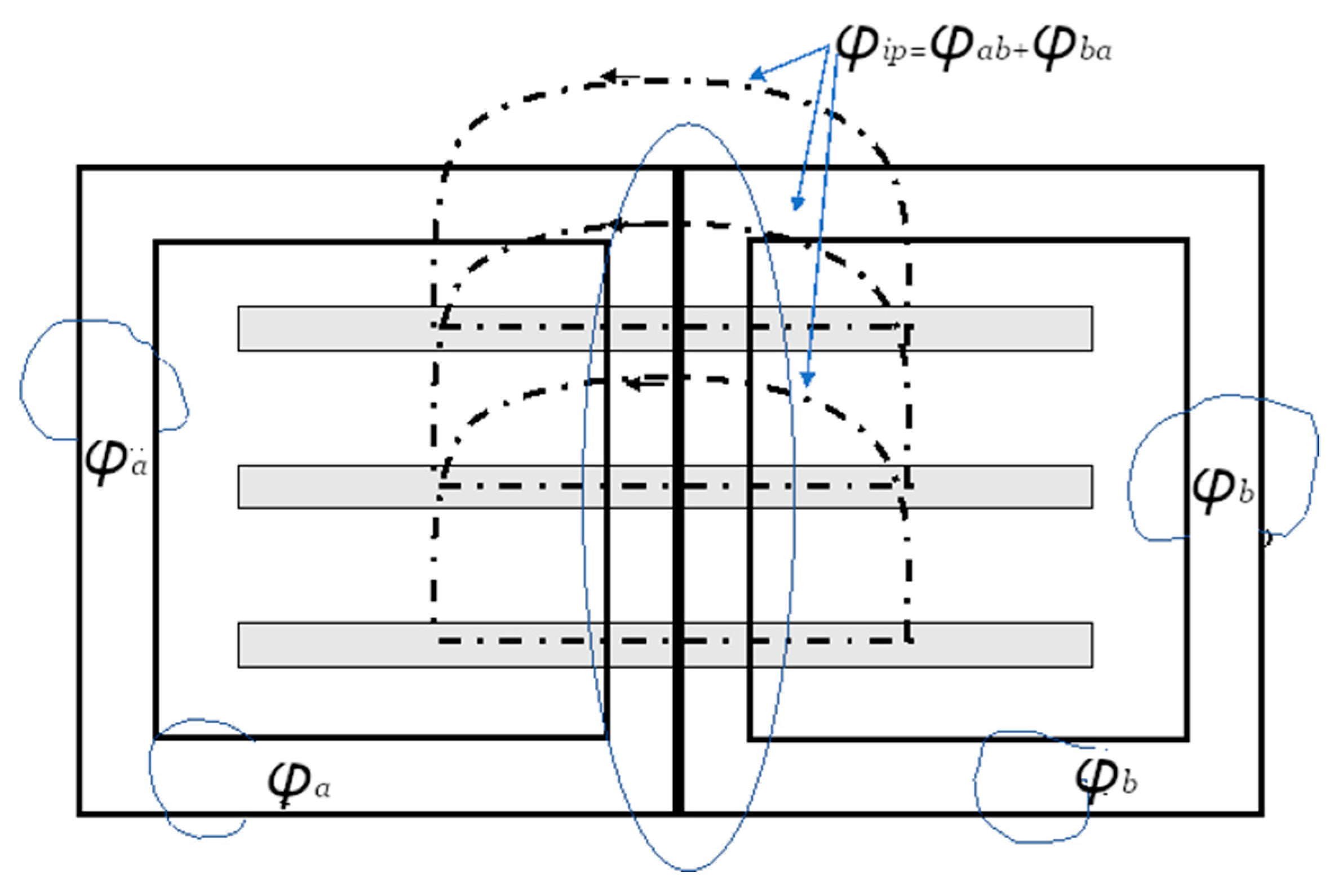
Based on the topology of the single-sided coupler, a new pad, denominated DD pad, was introduced in Reference [21] by researchers at the University of Auckland. This pad, shown in Figure 4, is composed by two coplanar D-shaped coils connected in series but wound in opposite directions.
As a direct result of this design choice, the coupler generates two magnetic fluxes that progress in opposite directions on the same side, making the pad a bipolar topology with the north and the south pole on the same face. A bipolar pad has its magnetic flux distributed in the area above it so that the coupling can be increased. In particular, the DD topology has coils electrically connected in parallel and magnetically connected in series (as shown by the behavior of ). It also has a region that is comparable to a flux pipe (see the shadowed portion of Figure 4). As a result, the structure combines the advantages of both the flux pipe coil and the circular pad. This feature enables this pad to work at a high efficiency rate when coupled with another DD pad and with a large magnetic flux distribution area, without requiring a large amount of shielding. Thus, the substantial benefits of this topology are preserved. The choice of two D-shaped coils for this pad is due to the mutual magnetic flux between couplers being proportional to the length of the intrapad area (the part with similar features as a flux pipe), and thus its length is maximized. In order to reduce the use of copper, the length of the coil is minimized, making the overall shape of the pad similar to a double D coil. The choice of the pad’s length and width and the amount of copper used were investigated in Reference [21], where two coils with different pitches were analyzed. Each pitch had varied proportions of ferrite strip covered by the coil, (called coverage of the midsection), that affected the overall length of the flux pipe of the pad and ultimately the behavior of the couplers. A narrow coil with low turns and low pitch has the same effect as a short flux pipe with low coupling factor and low flux leakage. On the other hand, a larger pitch results in a high flux leakage, which is inappropriate/undesirable for our application. Increasing the number of turns cannot be considered a solution because it tends to cause the inductance to reach an overly high value. The highest coupling factor was attained for coverage of 45% to 50% while the highest uncompensated power was obtained for coverage of 25%. For applications that required the exchange of 2 kW at an air-gap of 200 mm, two main coils were chosen as the most performant: one with 20 turns and coverage of 40%, and another coil of 22 turns and a coverage of 58%. The main difference between them was high-uncompensated power for the 22 turns coil and a lower self-inductance for the 20 turns coil. The pad’s dimensions were instead set depending on the number and length of the ferrite strips used to improve the path of the magnetic flux. For the previously mentioned application, a width of 430 mm and a length of 740 mm were set in order to ensure the maximum coupling with a minimal use of copper and ferrites.
Another feature of this topology is that when coupled with another DD pad, each section of the primary coil is linked with the corresponding section of the secondary coil, and the voltage at the pick-up terminals is the sum of the voltages induced in the two sections. Despite its great advantages compared to the other topologies, the DD geometry has some drawbacks that emanate from its magnetic flux symmetry. The magnetic flux distribution area of this pad has two main symmetries: one orthogonal to the intra-pad area, called x-direction, and one parallel to the intra-pad area, called y-direction. This particular distribution makes the topology unsuitable for an interoperable application, such as coupling with a radial symmetrical distributed flux like that generated by the circular pad. Furthermore, due to its bipolar behavior, the pad has a null point when misaligned in the x-direction, at 34% of its length. This is due to the transmitter being linked with only one section of the receiver without inducing a voltage and, as a result, it makes this topology unsuitable for applications that are characterized by huge x-axis misalignment [25,26,27,28,29].
2.4. DDQ Pad
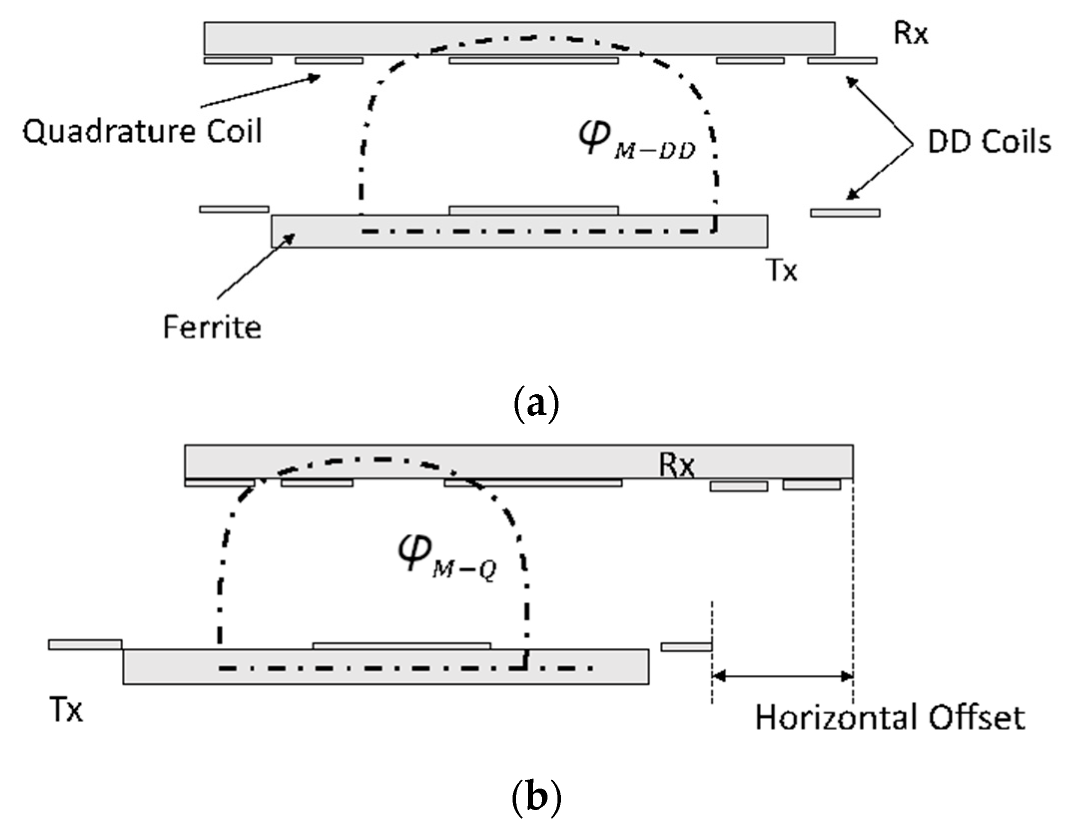
All the magnetic couplers introduced earlier have a good coupling factor when perfectly aligned, but in cases of misalignment, their magnetic behaviors decrease the system’s overall efficiency. This problem makes them not ideal for an application where misalignments are ordinary, such as applications for DWC systems where the vehicle is constantly moving upon the track. While compensation circuits can be introduced to mitigate the effect of misalignments on the coupling factor, for cases like the DD pad in which null points are present for misalignments, it is necessary to introduce other geometries of the pads. Starting from the DD pad topology that is characterized by the best coupling factor and the greatest magnetic flux distribution area of the presented pads, the researchers developed a new geometry that consists of the traditional DD coil with another coil added in quadrature, and which for this reason is denominated DDQ pad [30,31]. The DDQ pad (shown in Figure 5) benefits from the insertion of a quadrature component that is magnetically decoupled from the DD coil. This allows for independent control and tuning of both the coils though power converters and the capacity to capture the vertical and tangential flux component with the result of an improved misalignment tolerance [31].
The quadrature coil is positioned under the DD coupler and it only couples with flux that has an x-axis direction. In view of the traditional DD pad having a good coupling factor for y-axis components of the flux but a poor tolerance for misalignment on the x-axis, the addition of the quadrature coil enables the DDQ pad to overcome the main problems addressed from the double D coupler. Figure 6a shows that when a DDQ receiver is coupled and centrally aligned with a DD transmitter, the flux pattern remains unchanged and equal to the outcome of a DD receiver. The real difference can be seen in Figure 6b, where the null point for the DD coils is shown. In this position, instead of having zero coupling, we have a mutual flux that couples the DD coil at the primary side and the quadrature coil at the secondary side.
The overall performance of the coupler is determined by a combination of the DD coil and the added quadrature coil, which can be controlled separately using the power converters. Thanks to this feature, with the DDQ pad, it is possible to control the current in the double D coil and in the quadrature coil independently, allowing the overall coupler to be tuned depending on whatever geometry is used as the transmitting coil [32,33]. For these reasons, this pad is particularly suitable as a receiver in a DWC application in which the transmitting geometries can change, depending on the track section that the EV is running across. The DDQ magnetic coupler is also characterized by efficient use of the material employed compared to the more traditional rectangular and circular pads. Despite the efficient use of the material, the overall amount of copper used is extremely high, making the pad expensive compared to the other geometries [16,19,21]. While the cost of this coupler is not a big problem, since it is preferred as a receiver installed only on the EV and not all along the energized track, researchers have been interested in finding an alternative that can achieve the efficiency of the DDQ pad with less use of the materials.
2.5. Bipolar Pad
The University of Auckland achieved this goal with the introduction of a coupler called bipolar pad (BPP), which comprises a variation of the DD pad in which the two coils are increased in size and an overlap exists is created between the coils. This coupler, shown in Figure 7, does not have a fixed dimension for the overlap, but it is designed in order to have a mutual inductance equal to zero between the two coils.
This design choice reduces the use of copper by 25% compared to the DDQ pad [14,31], thus reducing the overall cost. Thanks to the absence of the mutual inductance, this pad can have two converters that independently tune the coils, just like the DDQs. This increases the inter-operability of the system.
Overall, these last two topologies of the magnetic coupler are the most suitable for DWC applications because of the requirement for good tolerance of misalignment on the x-axis and high inter-operability. In particular, the DDQ pad has the highest efficiency and the best performance, especially as a receiver, while the bipolar pad can be seen as a less expensive option that is capable of emulating almost the same performance as the DDQ.
3. Design of the Pad Prototypes
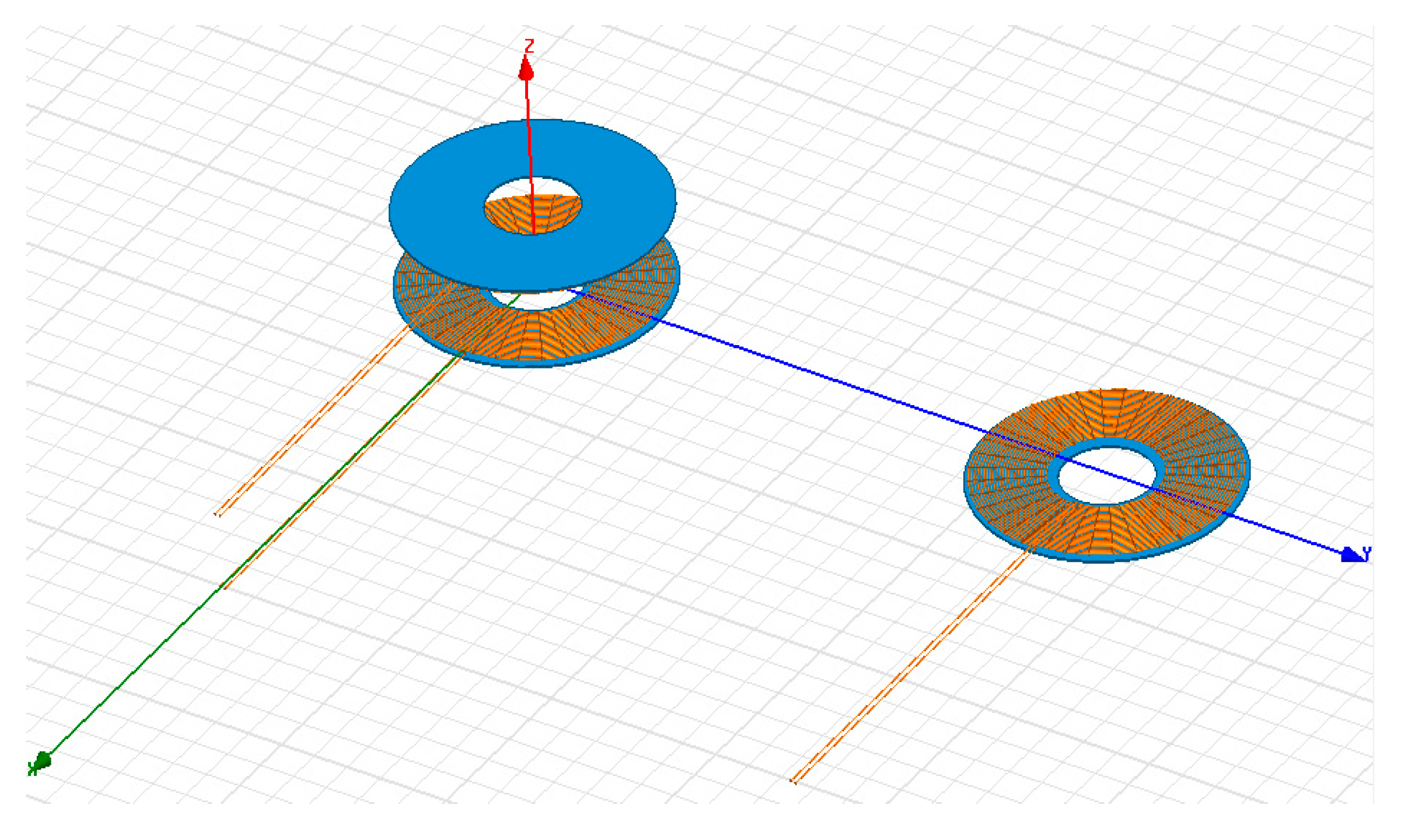
The objective of the analysis is to use the finite element method approach for a preliminary study of the best pad configuration that can be applied for a DWC with a lumped track. The geometries that are modelled and analyzed in ANSYS® Maxwell are the circular pad, the double-D pad, and the DDQ pad. These pads are at first coupled in a homogeneous way, such as a CP–CP configuration, and then are combined in order to obtain the different values of the coupling coefficients that will help us in the choice of the best configuration. The computing machine chosen for the simulations is an Asus® ROG with an Intel® core i7700 3.6 GHz processor, 16 Gb of RAM, and a dedicated GTX 1050 4 Gb graphic card. Before the start of the analysis, it is necessary to define the method and the procedure used in the design of the models for the simulation. The idea is to study the change in the coupling factor when the receiving side (Rx) is moving upon two different pads in the transmitting side (Tx), as shown in Figure 8.
These pads, whose characteristics are reported in Table 1, have a design that can be challenging for a computing machine, especially because the building of the mesh for the coil that is characterized by a short distance between every turn is complex and time-consuming. Consequently, it is necessary to make some assumptions and simplifications that can make the simulations less challenging and faster.
A first assumption can be made starting with an analysis on how the Rx pad moves along the track. The power exchanged between the primary and secondary sides is expressed as follows:
where and are the mutual inductances between the pick-up coil and the two respective transmitting coils, is the load attached to the pick-up coil, is the current that flows in the transmitting coils, and is the angular frequency of the current. From the expression it is highlighted how the power exchanged between couplers depends on the mutual inductances that are a function of the distance x. The mutual inductance is composed of two terms: a first one that represents the static component, which is also called transformer component, and a second one that represents the motion component, which is a function of the distance x. As demonstrated in Reference [12], the motion component is negligible when compared to the transformer component. Therefore, it is not necessary to perform a simulation with a transient solution, which requires more computational power. However, it is possible to perform a sweep-analysis with an eddy current solution, where the distance between the Rx and the Txs along the x-axis is changed with the start when the receiver is perfectly aligned with the first transmitter and the stop when the receiver is perfectly aligned with the second transmitter. Moreover, there is the possibility to perform a further simplification by changing the geometry of the pads, making them less difficult to mesh for the computing machine.
According to Ampere’s law, the magnetic field is related to the current density (J) in the coil and not with any geometric parameter:
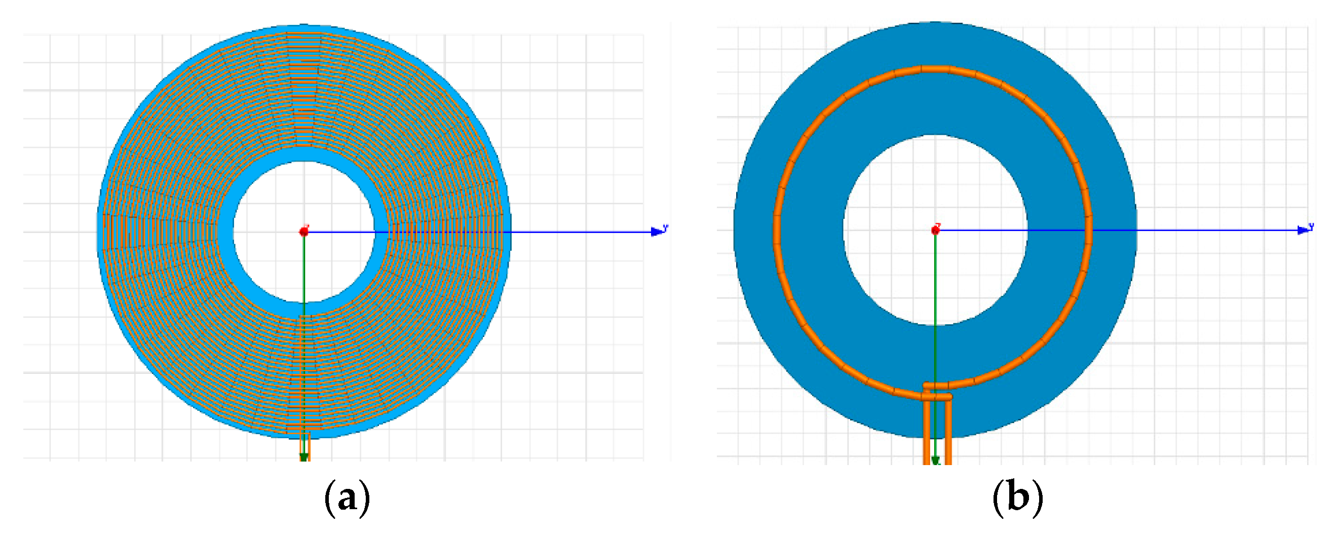
Therefore, it is possible to simplify the pads used in the simulation by substituting the 20-turns with 4 mm of copper wire diameter pad with a new one consisting of a single turn that can grant the same current density as the previous one, as shown in Figure 9.
The new pad will have then a radius equal to 8.95 mm due to the following relation:
where is the radius of the conductor of the new pad, is the radius of the conductor of the previous pad, is the area of the section of the conductor of the new pad, and as last is the total area of the section of all the conductors of the old pad.
Furthermore, in order to grant the same total current density in both the cases, it is necessary to increase the excitation current of the new and simplified CP up to 400 A. With a wire of this size, it is necessary to take into account that the eddy effect and the displacement currents would reach high values and, as a consequence, their effect will be removed from the simulation. The drawback of this design choice is that the mutual and auto inductances that will be computed by ANSYS® Maxwell are not the same as the original pads that would be used in a real scenario. This can be easily verified by observing the expression of the inductance of an ideal solenoid:
where is the permeability of the material, is the number of turns of the coil, is the area of the section of the coil, and as last, is the length of the coil.
As it can be seen, the inductance is proportional to the square of the number of turns, and as a consequence the simplified pad proposed, due to the fact that it is characterized by a single turn, has a value of the inductances that is approximately reduced by a factor of 202 when compared to the real case. Despite this, the simplifications do not affect the coupling coefficients that will be obtained, because of its independence from the number of turns making the results coherent and close to the values found in the literature.
All the pad topologies that are analyzed in the simulation are subject of the assumptions and simplifications outlined in the previous paragraph. Other important parameters that define all the models are: (i) the air-gap between the transmitting and receiving side, (ii) the distance between the transmitting coils, and (iii) the position of the receiver along the moving direction, also called Offset. The air-gap was set to 200 mm, which is inside the common vehicle range of 175–220 mm gap, and which ensures the minimum gap for the safety operations of 10 cm. Regarding the distance between the transmitting coils, a distance greater was chosen than the dimension of the pad on the moving direction, so that the mutual inductances between the coils could be neglected, as reported in Reference [16]. Considering a diameter of 700 mm for the pads, the distance was set to 1 m because it represents a good trade-off that can guarantee enough distance to have a low coupling factor between transmitting coils, while having a uniform power transmission. As last, the Offset parameter was set as an array of discrete values that will simulate the position of the Rx along the moving direction. This analysis is called sweep-analysis and it was chosen due to the decision to neglect the motion component of the mutual inductances. The excitation current of all the pads that will be simulated is 400 A for both the transmitter and the receiver side. Finally, the operating frequency set in the solver was 20 kHz, and the chosen solution type was the eddy current solution that will give us the values of the coupling coefficients for every step of the Offset once the simulation is over.
4. Results and Discussion
In this section, the results obtained for six pad configurations that can be utilized for a DWC with a lumped track are reported. These consist of the coupling coefficients for each configuration and their trend as a function of the Offset and Lateral Misalignment.
4.1. CP–CP Configuration
In Figure 10, the values of the coefficient k for all the computed values of the Offset are reported, then a first analysis of the results can be performed. It can be seen that for a value of the Offset equal to zero, i.e., when the Rx pad is perfectly aligned with the first Tx pad, their coupling coefficient k(Tx1) has a value equal to approximately 0.154, which is a value close to the results obtained in Reference [20].
When the Offset starts to increase, the coupling coefficient decreases its value rapidly, reaching the value of zero at 0.5 m, leaving the receiver pad decoupled from any source of power until the Offset reach the value of 1.15 m, where the Rx starts to couple with the secondary transmitter k(Tx2). In Figure 11a, the magnitude of B is plotted on the XY section between the couplers, and it highlights how the magnetic flux does not spread either on the x or y-axis but has a vertical symmetry and a focused vertical distribution, an observation supported also in Figure 11b.
This makes the overall distribution area pretty small, which therefore causes the coupling coefficients of the pads to significantly drop when they are not perfectly aligned. From the obtained results, it is clear that a CP–CP configuration, while capable of reaching a good coupling factor at a 200 mm air-gap for a WPT application, has poor behavior when the couplers are misaligned, making the configuration not the best choice for a DWC system, where the couplers are misaligned most of the time.
4.2. DD–DD Configuration
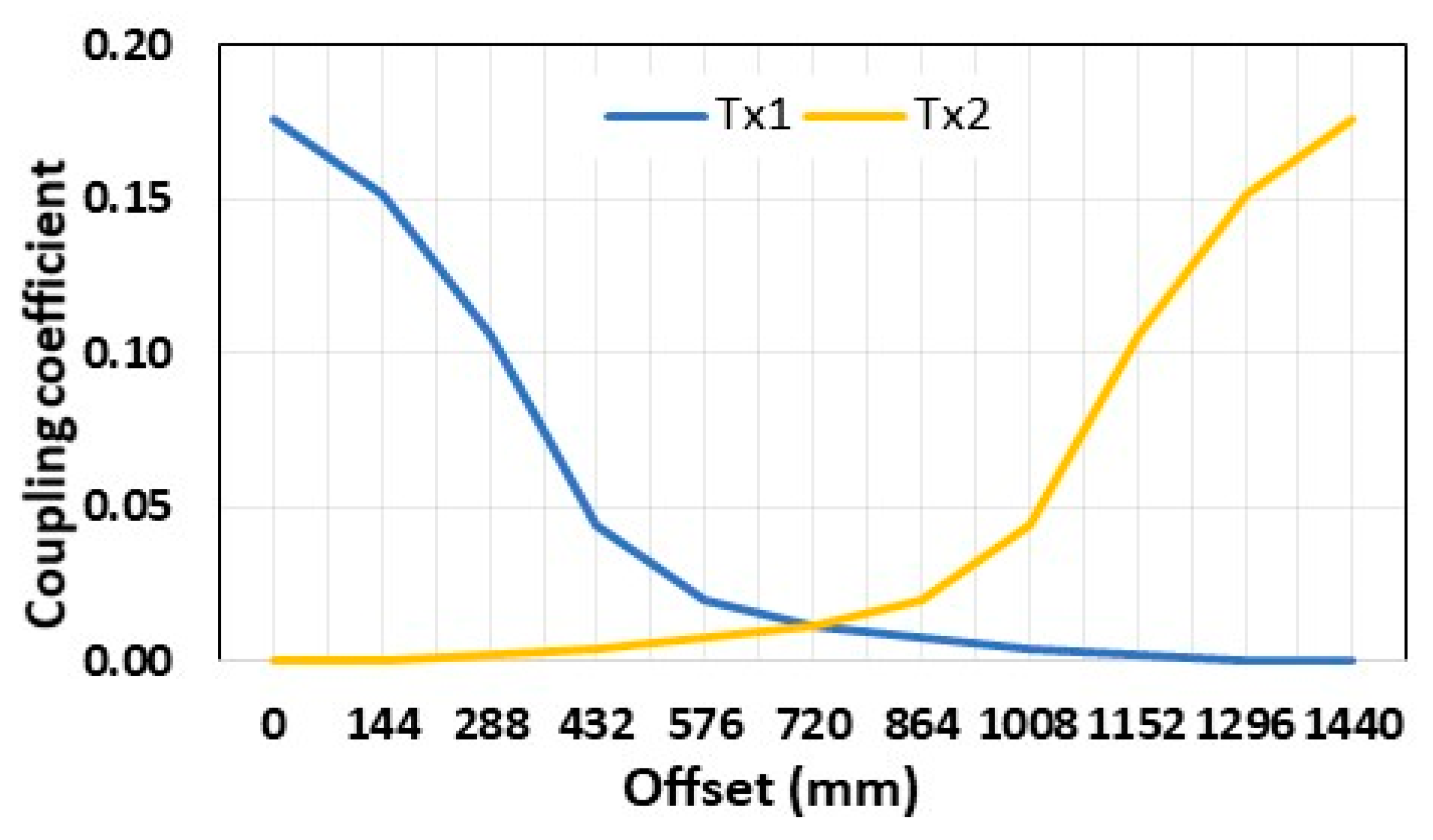
Figure 12 shows the model of the 720 × 440 mm size DD pad used for the simulations. The simulation results reported in Figure 13 confirm the better behavior of the DD pad for a dynamic wireless power transfer application. When perfectly aligned, the coupling coefficient between Tx and Rx, called k(Tx1), has a value of approximately 0.176, which is higher than that obtained in the CP–CP case. Furthermore, when the value of the Offset increases, the coefficient k does not considerably drop as in the previous case, allowing a more homogeneous power exchange between the transmitting and receiving side because there are no points in which the receiver is completely decoupled from both the first and the second transmitter.
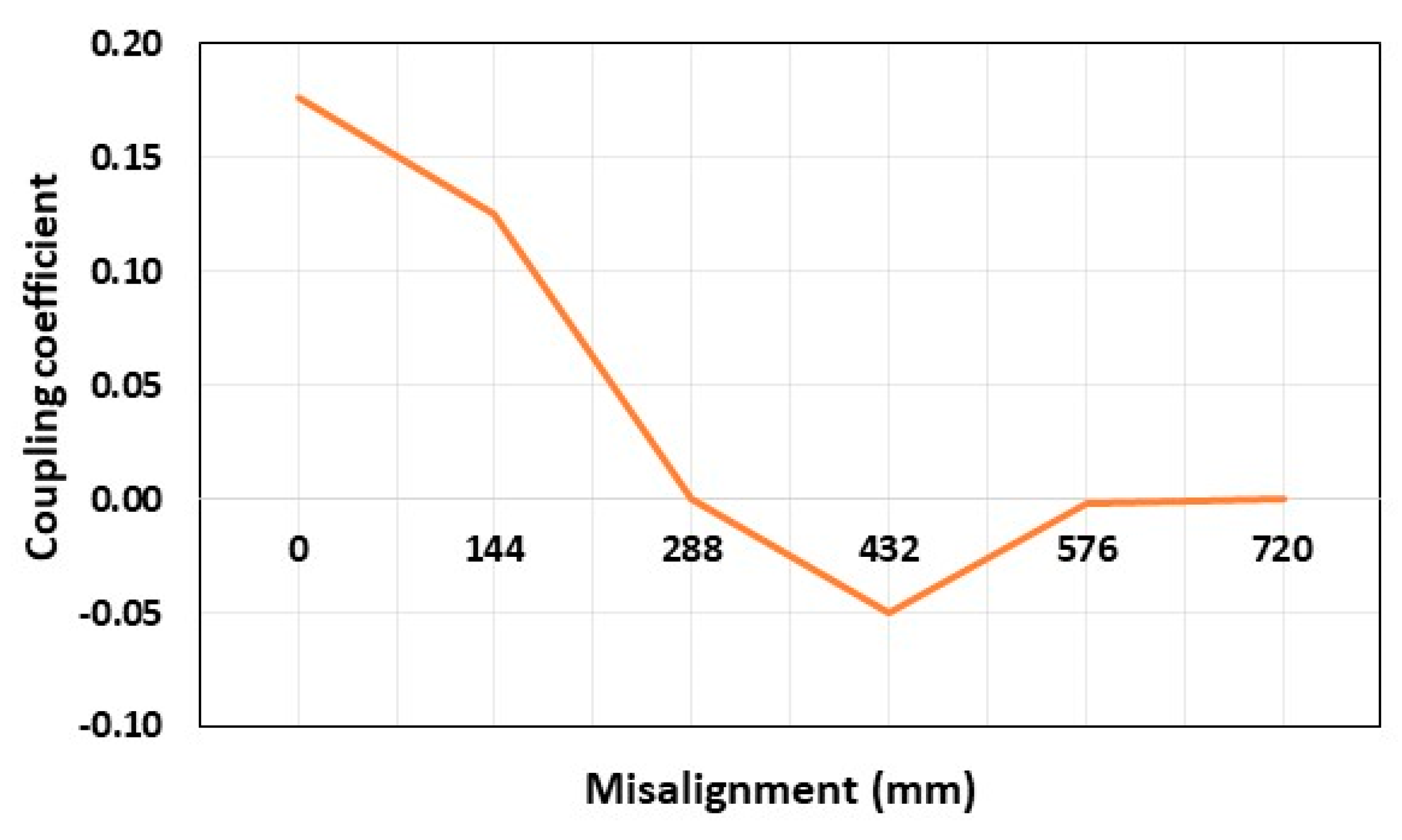
Figure 14 presents the plot of the coupling coefficient as a function of the Lateral Misalignment. It can be seen that the coupling factor has a null point at around 40% of the length of the pad, a value that differs from the 34% found in the literature. This difference is due to the simplified model adopted in the numerical simulation, with also a different geometry having a slight effect on the results obtained.
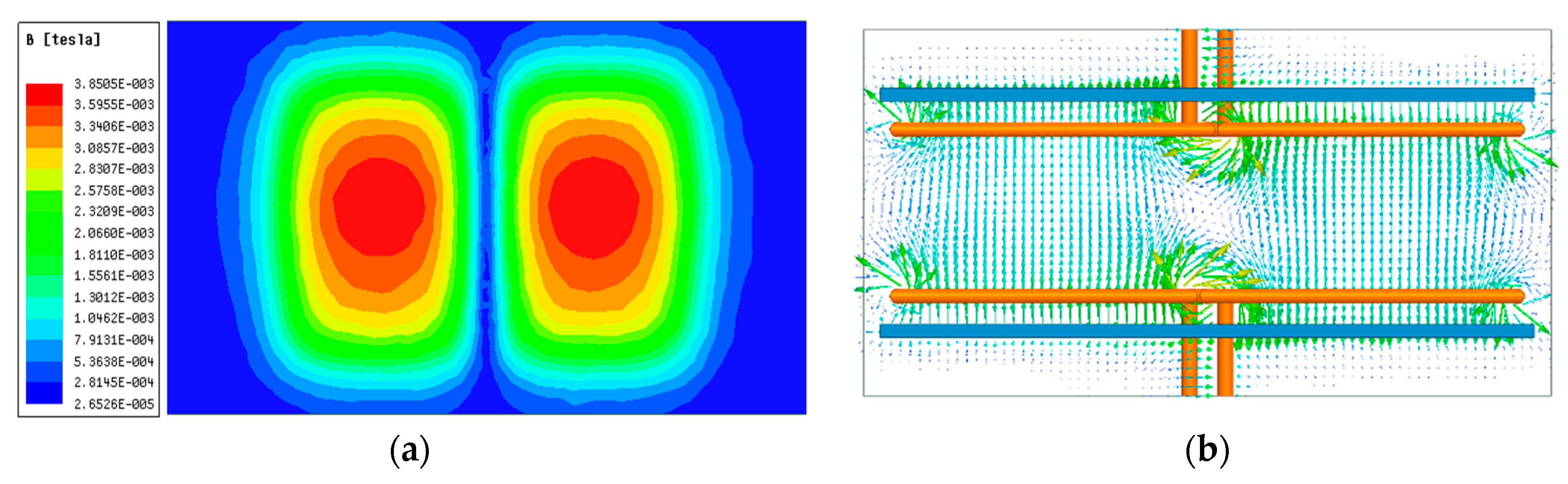
Moreover, based on the distribution area of the magnetic field depicted in Figure 15a, it can be seen to have improved when compared with the CP–CP case. From this, it follows a greater charge area for the pad and better behavior when the pads are not aligned. Another important characteristic of the DD pad can be studied starting from the plot of the B-vector illustrated in Figure 15b, where the bipolar behavior and the flux-pipe intrapad area can be easily recognized.
Note that in our model, the intrapad area does not have a high contribution due to its reduced size, which is a consequence of the reduction in the number of turns, but it can still be observed how this pad can behave like a composition of two circular pad and a double-sided flux-pipe pad. Regarding the bipolar behavior of the coupler, the latter generates a stronger B field in the area above the pad, which results in a higher coupling factor; however, it decreases the Lateral Misalignment tolerance (along the y-axis).
4.3. DDQ–DDQ Configuration
Figure 16 presents the simplified model implemented in the simulations. This model differs from the previous DD pad because it has in addition a quadrature coil with a 500 × 440 mm2 size.
Figure 17 shows the simulation results of the evolution of the different coupling coefficients as a function of the Offset. As expected, the values of the coefficient k between the DD coil of the receiver pad and the DD coil of the transmitting side (Tx–Rx(DD–DD)) follow the same trend obtained for the DD–DD configuration. It is interesting to note that in addition to the DD–DD contribute, there is now also the Q–Q contribution (Tx–Rx(Q–Q)) that increases the overall efficiency of the exchange of power. This new contribution has a value of 0.10 at its peak, and it reaches the value of zero faster when compared to the DD–DD one, but it has been added mainly to increase the power exchange when there is a Lateral Misalignment between pads. Moreover, it can also be seen how the DD–Q contribution (Tx–Rx (DD–Q)) can almost be neglected because the flux that the quadrature coil generates is collected by the DD coil in a symmetrical way, and as a consequence, the flux that interacts with the positive pole is the same as the flux that interacts with the negative pole, making then the overall collected flux at the DD coil close to zero.
This can be noticed in Figure 18a, where it can be seen that the pole of the DD coil of the receiver couples in a constructive manner with the Q coil of the transmitter. The other pole couples in a destructive way, decreasing the magnitude of the B field, because the vector of the field generated by the DD and Q coils have the same direction but on an opposite verse, as shown in Figure 18b.
Another important analysis can be done based on the results shown in Figure 19, where the trend of different coupling factors as a function of the Lateral Misalignment is presented.
As expected, the coupling factor between the DD coil of the Rx and the DD coil of the Tx (Tx–Rx (DD–DD)) has the same behavior of the DD–DD configuration presented in Figure 6. The Q–Q contribution (Tx–Rx (Q–Q)), while having an effect on the power exchange for perfect alignment, does not have an important contribution on the Lateral Misalignment because the coefficient k reaches the value of zero almost at the same distance as for the Tx–Rx (DD–DD). What make the DDQ pad more performant than the DD pad, when there is a Lateral Misalignment, is the DD–Q contribution (Tx–Rx (DD–Q)) that keep the Tx and Rx pads coupled for a wider range of Lateral Misalignment values, reaching the value of zero for a Lateral Misalignment of 625 mm. This proves that the quadrature coil added to the DD coil has an important effect on the performance of the pad, making it more efficient when misaligned and improving the overall coupling coefficient value of the pads, with a consequent increase in the efficiency of the system.
4.4. CP–DD Configuration
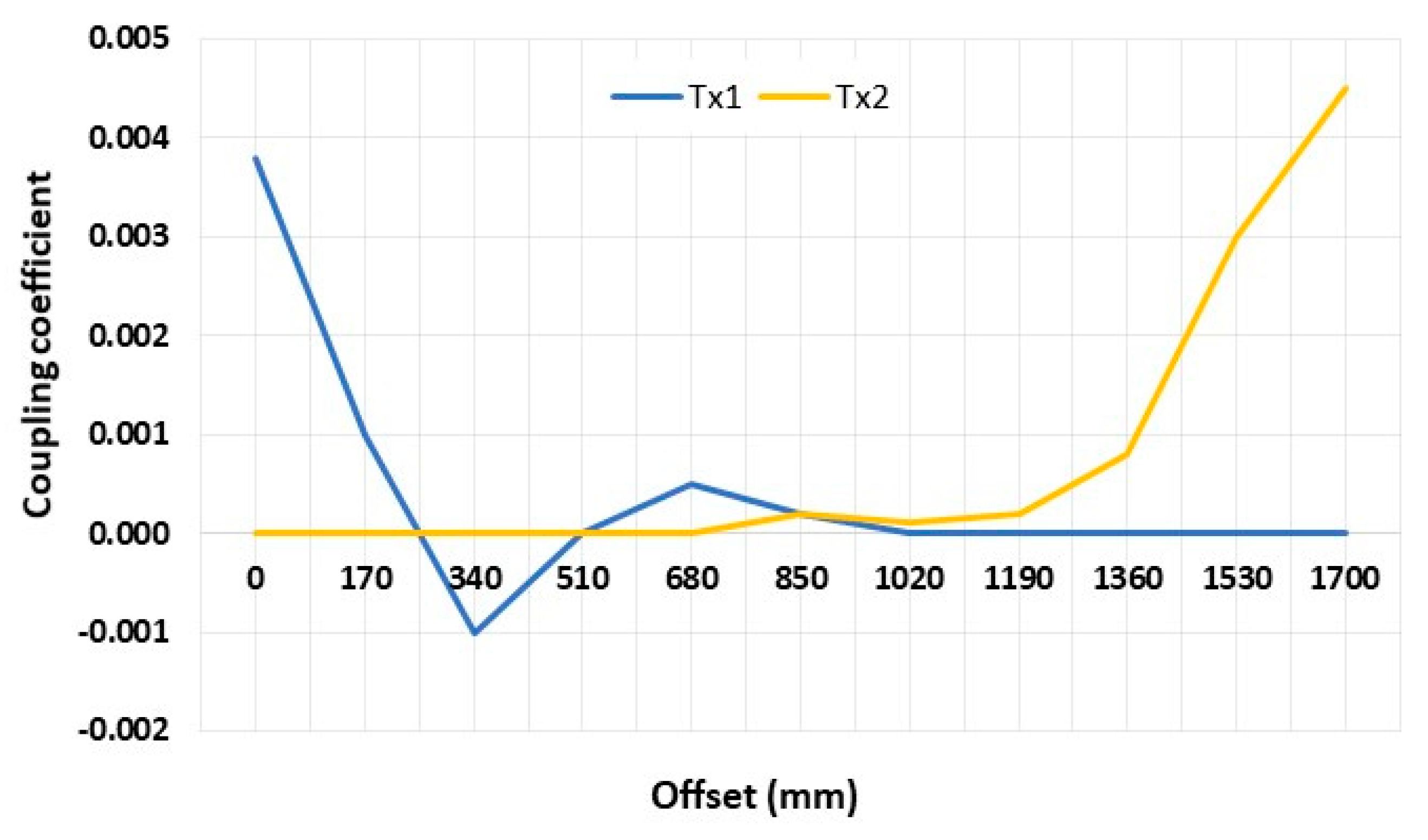
Now that all the modelled pads and their features have been introduced, it is time to perform analysis with mixed configurations, which means, two different geometries for the Tx and the Rx. The goal is to analyze all the possible configurations with the introduced pads, in order to find the most performant one for a DWC application. The first combination that is analyzed is the CP–DD configuration, where a circular pad is used in the transmitter array and a DD pad is used as a receiver. The results of the simulation are depicted in Figure 20. From the plot, it can be seen that the coupling coefficient between the receiver and the first transmitter, called k(Tx1), has a value of 0.004, which is very low when compared to the previous results, even when the pads are perfectly aligned.
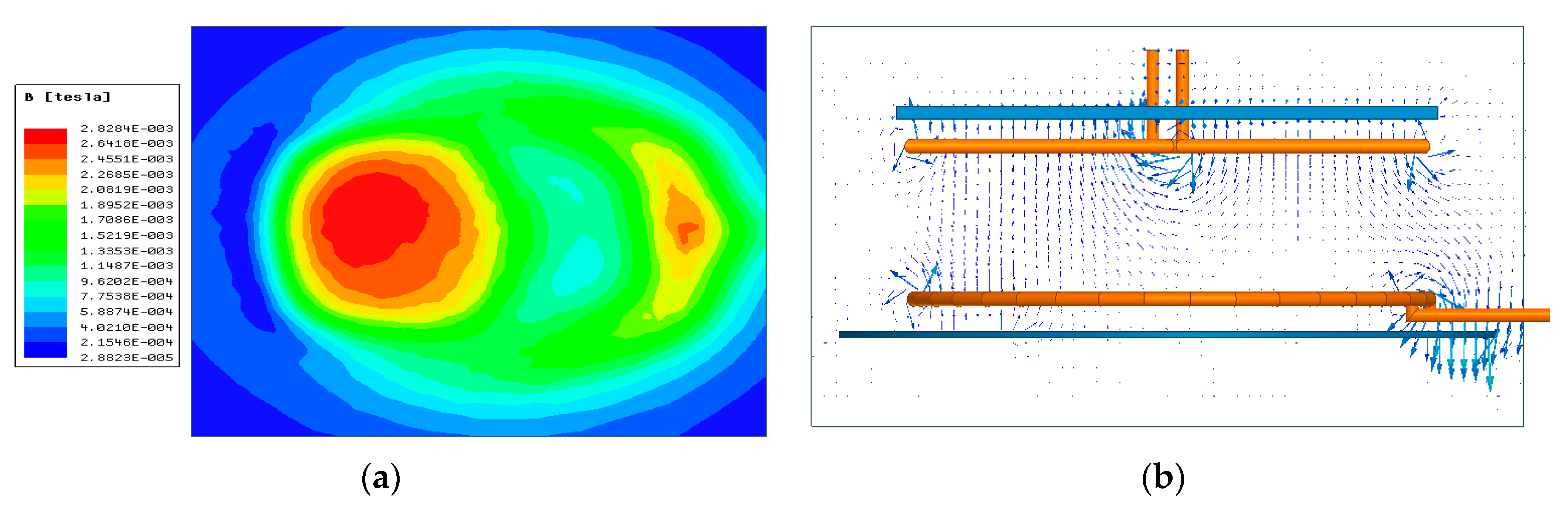
The same outcome is true also for the coupling coefficient between the receiver and the second transmitter, which slightly differs from k(Tx1) because the simulation did not reach the convergence in all the Offset values. These results show that it is clear that this configuration is not suitable for a wireless power transfer application, neither for a static nor for a dynamic one. The reason of the low coupling coefficient is that the magnetic flux generated by the CP pad is collected from both the positive and negative poles of the DD pad in an equal manner, making the resultant magnetic flux collected close to zero. This can be seen in Figure 21, where the interaction between the pads is noticeable and the constructive coupled pole can be distinguished by the destructive coupled pole.
Overall, the performance of the CP–DD configuration can be considered negative and not suitable for a WPT application because of the low coupling factor, making the exchange of power not efficient.
4.5. CP–DDQ Configuration
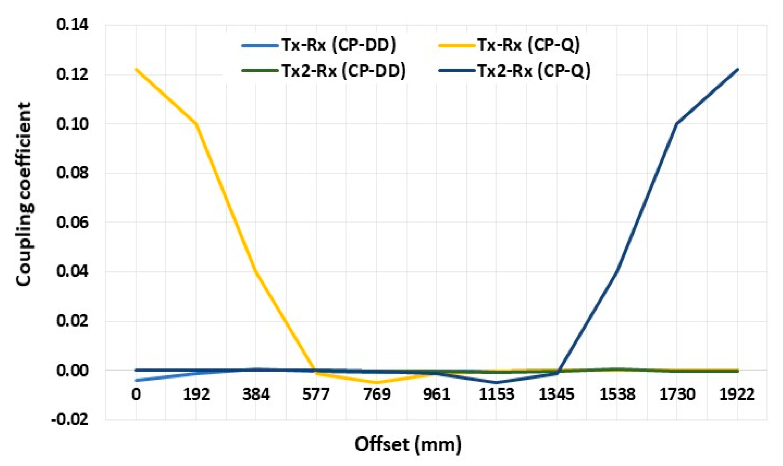
The configuration that will be analyzed next is the CP–DDQ configuration, where the circular pad is used for the transmitter array while the DDQ pad is used as a receiver. The results of the sweep-analysis are depicted in Figure 22 and shows that there are two contributions that describe the coupling behavior between pads: a first term that describes the CP–DD coupling and a second term that describes the CP–Q coupling.
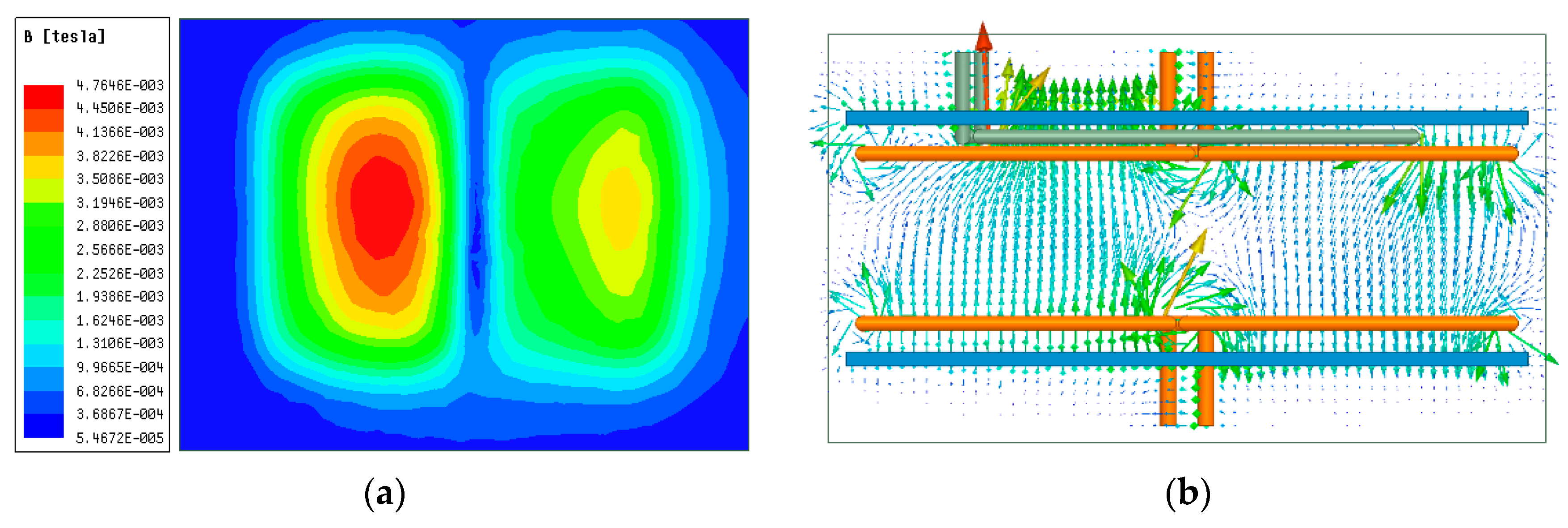
As obtained in the DD–CP and in the CP–DD cases, also in this configuration, the CP–DD term has a value that is close to zero for every step of the analysis, which means that it does not have a real contribution in the power exchange. On the other side, the coupling coefficient between the first transmitter and the quadrature coil of the receiver, called Tx–Rx (CP–Q), has a value close to 0.13 when the pads are perfectly aligned. This value rapidly decreases when the value of the Offset starts to increase, reaching the value of zero for an Offset of 0.55 m. The receiver will start to couple with the second transmitter for an Offset of 1.35 m, leaving then the secondary pad without any coupling source for a distance of 0.8 m. The improvement in the coupling between pads can be seen also in Figure 23, where the magnitude and the vector plot of the B-field are shown. The plot in Figure 23a shows a similar distribution area observed in the DD–CP and CP–DD cases, with the difference of an improvement in the magnitude of the field. In the area between the constructive poles, the magnetic field reaches now the value 3.711 × 10⁻³ T, while in the CP–DD case the value was 2.8284 × 10⁻³ T. The vector plot of the field, seen in Figure 23b, is overall similar to the one obtained in the DD–CP and CP–DD cases, which means that with a higher magnitude of the B-field and the same area of the surface, the magnetic flux chained to the receiver is improved. This improvement of the magnetic flux has an effect in the induced voltage, which in turn has an effect in the power at the secondary side of the system, the receiving side.
One last analysis can be performed on the misalignment tolerance along the y-axis of the configuration; the values of the coupling coefficient as a function of the misalignment are shown in Figure 24.
From the Figure 24, it can be seen that the coupling coefficient between the transmitter and the DD coil of the receiver, called Tx–Rx (CP–DD), has a value of zero when the pads are perfectly aligned, but it reach a value of –0.09 for a misalignment of 0.4 meters. This contribution has a negative effect on the coupling between pads because for a misalignment value of 0.4 meters the CP transmitter is coupled mainly with the positive pole of the DD coil, which has a destructive effect on the coupling coefficient, as already shown in the analysis of the B-field distribution between the pads. A solution could be to tune the current that flows in the DD pad of the receiver in order to decrease its value when the pads are misaligned and decrease, therefore, the negative effect of the coupling factor between the CP and DD coils. The coupling coefficient Tx–Rx (CP–Q) between the transmitting pad and the Q coil of the receiver has instead a value of 0.13 when the pads are perfectly aligned, and it decreases until it reaches a value of zero for a misalignment of 0.4 meters. Therefore, it can be stated then that the CP–DDQ configuration is characterized by a flexible behavior that allows the exchange of power when the pads are misaligned along the y-axis, but it is necessary to avoid the destructive contribute of the Tx–Rx (CP–DD) by the appropriate control of the currents in the DD coil of the receiver.
4.6. DD–DDQ Configuration
The final configuration examined is the DD–DDQ configuration, where the primary array is composed of DD pads and the receiver is the DDQ pad, all of them with the size introduced in the previous cases. The results obtained from the simulation for every step of the Offset are depicted in Figure 25.
As shown in Figure 25, the trend of the coupling factor between the DD coil of the receiver and the first transmitter, called Tx–Rx (DD–DD), is equal to what obtained in the DD–DD case, with a peak value of 0.18 when the pads are perfectly aligned. In addition, the coupling coefficient Tx2–Rx (DD–DD) follows the same trend as for the DD–DD case, allowing the receiver to be coupled with the transmitting pads for every step of the Offset, because of the x-axis misalignment tolerance of the pads. It is also important to highlight that the results are close to the DD–DD pad because the interaction between the DD and Q coils of the receiver is minimized due to its geometric design. Furthermore, the results give us also information on the coupling coefficients between the Q coil and the transmitters, which are characterized by a value close to zero for every value of the Offset. This lack of interaction between the quadrature coil and the DD pad used as a transmitter can be explained starting from an analysis of the magnetic field distribution between the pads. Figure 26a shows the distribution of the B-field along the XY section between the pads, and it highlights the bipolar behavior of the pads used. A particularity is that one pole is characterized by a higher magnitude of B-field when compared to the other.
This is because one pole couples in a constructive way with the quadrature coil while the other couples in a destructive way with the quadrature coil, similar to what happened in all the previous cases with a bipolar pad used in the configuration. A further demonstration of the lack of interactions between the DD transmitter and the Q coil at the receiver is obtainable by the observation of Figure 26b, where the plot of the B-field vector over the YZ section is depicted. In the figure, the pole on the left can be distinguished, where the coils interact in a constructive way, and the pole on the right, where the pole is coupled in a destructive way. Starting from the definition of magnetic flux,
where is the area of the surface that chains the magnetic flux, it is easy to understand the effect of the DD coil on the quadrature coil used as a receiver. The amount of magnetic flux with positive direction chained to the area of the surface of the quadrature coil is equal to the amount of magnetic flux with a negative direction. The total magnetic flux chained ($tot$) is composed of two contributions, a positive and a negative one, which have an equal magnitude, making its value close to zero. With a null magnetic flux chained to its surface area, the induced voltage on the quadrature coil is zero, according to the Faraday’s law (Equation (5)), making the interaction between the DD coil and the Q coil equal to zero. In other words, the negative pole of the Q coil interacts with both the positive and negative pole of the DD pad in an equal measure, generating an area where the couple is constructive that has the same magnitude of the area where the couple is destructive, with a consequent overall coupling factor between these coils close to zero.
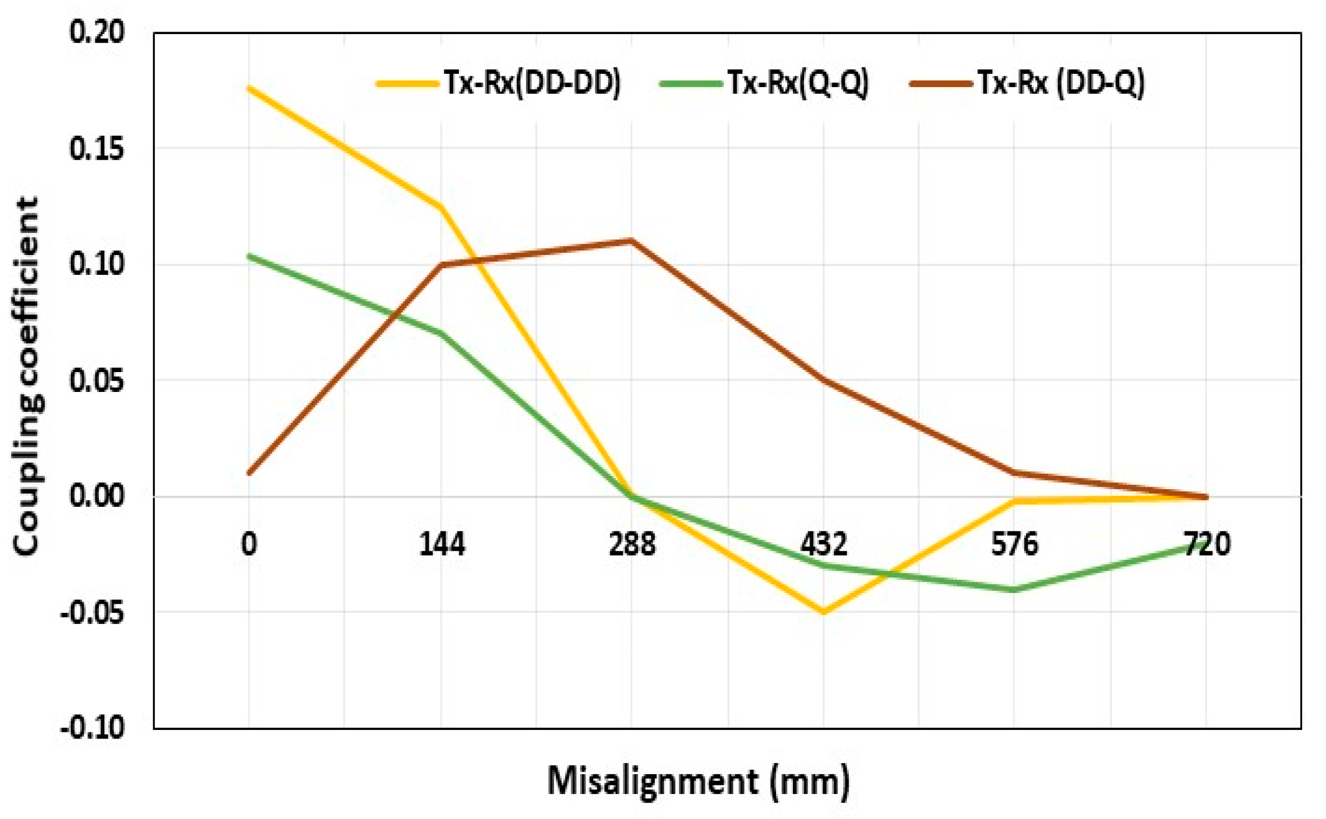
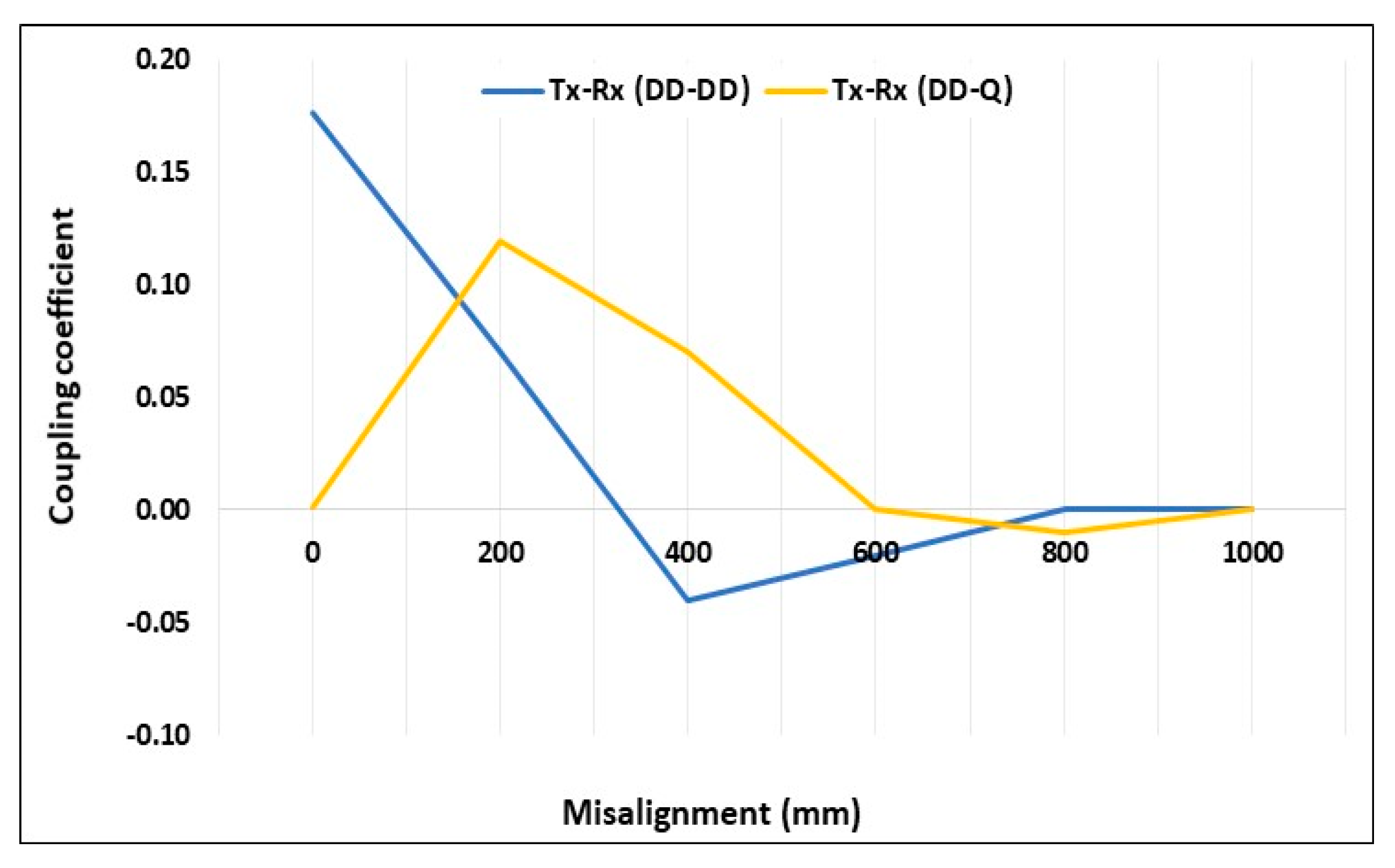
Now that the behavior of the configuration when the Rx pad is moving along the x-axis is determined, it is important to analyze also the performance when the pads are misaligned along the y-axis. The results of the simulation for different values of the misalignment are shown in Figure 27 and depict a trend in the coupling coefficient values similar to what was obtained for the DDQ–DDQ configuration.
The coupling coefficient Tx–Rx (DD–DD), which is the coupling coefficient between the DD pad of the receiver and the DD pad of the transmitter, reaches a value of zero for a misalignment of 0.320 meters. This value is lower than the one found for the CP–DDQ configuration and highlights the sensibility to the misalignment of the DD–DD coupling. The contribution of the coefficient Tx–Rx (DD–Q) between the quadrature coil and the transmitter is what makes this configuration efficient and performant also for high values of misalignment. Indeed, this coupling factor has a value close to zero when the pads are perfectly aligned, as previously discussed, but it increases its value for an increase in the misalignment, with a maximum around 0.200 m. After the maximum is reached, the value decreases with a zero point at a misalignment of 0.600 m, which is greater than the value obtained for the DD–DD component of the pad.
5. Conclusions
The results obtained from this analysis are useful to determine the design that is considered the best configuration for a DWC application. The CP–CP configuration is characterized by the lowest coupling factor when perfectly aligned, with a value of 0.154, and a non-optimal Offset and Lateral Misalignment tolerance. On the other hand, the design of the circular pad is easier, compared to the DD and DDQ pads, and its cost is not very high, making the CP topology a good option for the application to the WPT system. The main drawbacks of the CP–CP configuration are compensated in the DD–DD configuration, where the value of the coupling factor is now 0.176, and the Offset tolerance is highly improved. The Offset tolerance is particularly important for a DWC system because the Rx pad is often misaligned along the x-axis and as a result, the choice of the pad with a good Offset misalignment is considered crucial for a homogeneous power exchange. The DD pad is not the best choice because of its poor tolerance for Lateral Misalignment, which is even worse than that of the CP pad, with undesirable consequences on the power exchange if the Rx and Tx pads are misaligned along the y-axis. For this reason, the DDQ pad can be considered an improvement on the previous DD topology. Indeed, the addition of the quadrature coil ameliorates the misalignment along the y-axis due to the DD–Q interaction between the primary and secondary side. Therefore, the DDQ–DDQ configuration can be considered the most performant configuration, with a coupling coefficient DD–DD of 0.176, a coupling coefficient Q–Q of 0.10, and a good misalignment tolerance on both the x and y-axes. The main drawback of this solution is its higher cost and its complicated design. The DDQ pad uses more copper compared to the DD and the CP pads, and its main advantages originate from the fact that the DD and the Q coil are decoupled and can be tuned differently using different power converters. The need for two converters is what makes the DDQ pad expensive and for this reason, it is important to find a configuration characterized by the same behavior of the DDQ–DDQ one but with a comparatively lower overall cost. The first solution explored is the CP–DD configuration but, from analysis of the results, it is evident that this configuration cannot work for any WPT application. The use of a bipolar pad coupled with a unipolar pad results in a coupling factor close to zero, thus rendering the configuration unusable. When the DDQ pad is used instead of the DD one, the coupling coefficient now is composed of two components: the CP–DD component, which has a value still close to zero, and the CP–Q component, which has a value of 0.13. While the overall configuration still has the ability to work, the performance is not close to the DDQ–DDQ configuration due to a lower value of the coupling coefficient and a bad Offset and Lateral Misalignment tolerance. The last configuration used is the DD–DDQ one, where the DDQ pad is installed at the car’s side. The choice of the DDQ pad at the secondary side is for economic reasons. It is more convenient to install the DDQ pad at the secondary side because it requires more power converters and it is more expensive overall, and consequently, it would not be feasible to have an entire array track composed of these pads. Regarding the performance of the configuration, the coupling coefficient is also composed of two terms: a DD–DD term and a DD–Q term. The first term has a value of 0.176, as in the previous configuration, while the second term has a value close to zero for the same reasons as for the CP–DD configuration. The misalignment tolerance on the x and y-axis is really close to the results obtained for the DDQ–DDQ pad.
In conclusion, the results establish that the best trade-off between performance and economic feasibility is the DD–DDQ pad, which is characterized by the best values of coupling coefficient and misalignment tolerance, without the need for two power converters for each side, as in the DDQ–DDQ configuration.
Author Contributions
A.D. and M.L. proposed the core idea and developed the models. D.D.M. performed the simulations, exported the results, and analyzed the data. W.Y. revised the paper. D.D.M., A.D., M.L., and W.Y. contributed to the design of the models and the writing of this manuscript.
Funding
This research received no external funding.
Conflicts of Interest
The authors declare no conflict of interest.
References
- Ribeiro, S.K.; Figueroa, M.J. Global Energy Assessment-Toward a Sustainable Future; Chapter 9-Energy End-Use: Transport; Cambridge University Press: Cambridge, UK, 2014; pp. 586–611. [Google Scholar] [CrossRef]
- European Environment Agency. Total greenhouse gas emissions from transport. In Indicator Assessment Data and Maps; European Environment Agency: Copenhagen, Denmark, 2015. [Google Scholar]
- Moriarty, P.; Honnery, D. Global Transport Energy Consumption. In Alternative Energy and Shale Gas Encypledia; John Wiley & Sons, Inc: Hoboken, NJ, USA, 2017. [Google Scholar] [CrossRef]
- Garcia-Vazquez, C.A.; Sàanchez-Sainz, H.; Jurado, F. Evaluating Dynamic Wireless Charging of electric vehicles moving along a stretch of highway. In Proceedings of the 2016 International Symposium on Power Electronics, Electrical Drives, Automation and Motion, Anacapri, Italy, 22–24 June 2016. [Google Scholar] [CrossRef]
- US Energy Information Administration (EIA). Global Transportation Energy Consumption: Examination of Scenarios to 2040 Using ITEDD; EIA: Washington, DC, USA, 2017.
- Ban, J.; Arellano, J.; Alawami, A. 2016 World Oil Outlook; Organization of the Petroleum Exporting Countries: Vienna, Austria, 2016; pp. 24–204. [Google Scholar] [CrossRef]
- Vilathgamuwa, D.; Sampath, J. Plug in Electric Vehicles in Smart Grids; Springer: Singapore, 2015. [Google Scholar] [CrossRef]
- Rim, C.T. Wireless Charging of Electric Vehicles. In Power Electronics Handbook; Chapter 34; CRC Press: Boca Raton, FL, USA, 2018. [Google Scholar] [CrossRef]
- Kosmanos, D.; Maglaras, L.; Mavrovouiniotis, M. Route Optimization of Electric Vehicles Based on Dynamic Wireless Charging. IEEE Access 2018, 6, 42551–42565. [Google Scholar] [CrossRef]
- Bi, Z.; Kan, T.; Mi, C. A review of wireless power transfer for electric vehicles: Prospects to enhance sustainable mobility. Appl. Energy 2016, 179, 413–425. [Google Scholar] [CrossRef] [Green Version]
- Lukic, S.; Saunders, M.; Pantic, Z. Use of inductive power transfer for electric vehicles. In Proceedings of the IEEE PES General Meeting, Providence, RI, USA, 25–29 July 2010. [Google Scholar] [CrossRef]
- Buja, G.; Rim, C.T.; Mi, C. Dynamic Charging of Electric Vehicles by Wireless Power Transfer. IEEE Trans. Ind. Electron. 2016, 63, 6530–6532. [Google Scholar] [CrossRef]
- Rahmani, F.; Barzegaran, M. Dynamic wireless power charging of electric vehicles using optimal placement of transmitters. In Proceedings of the 2016 IEEE 17th Biennial Conference on Electromagnetic Field Computation (CEFC), Miami, FL, USA, 13–16 November 2017. [Google Scholar] [CrossRef]
- Xiang, L.; Sun, Y.; Tang, C. Design of crossed DD coil for dynamic wireless Charging of Electric Vehicles. In Proceedings of the 2017 IEEE PELS Workshop on Emerging Technologies: Wireless Power Transfer (WoW), Chongqing, China, 20–22 May 2017. [Google Scholar]
- Covic, G.; Boys, J. Modern trends in inductive power transfer for transportation applications. IEEE J. Emerg. Sel. Top. Power Electron. 2013, 1, 28–41. [Google Scholar] [CrossRef]
- Sabki, S.; Mei, N.; Tan, L. Wireless Power Transfer for Electric Vehicle. IEEE J. Emerg. Sel. Top. Power Electron. 2014. [CrossRef]
- Nagatsuka, Y.; Ehara, N.; Kaneko, Y.; Abe, S.; Yasuda, T. Compact Contactless Power Transfer System for Electric Vehicles. In Proceedings of the 2010 International Power Electronics Conference—ECCE ASIA, Sapporo, Japan, 21–24 June 2010. [Google Scholar] [CrossRef]
- Budhia, M.; Covic, G.; Boys, J.T. A New IPT Magnetic Coupler for Electric Vehicle Charging Systems. In Proceedings of the 36th Annual Conference on IEEE Industrial Electronics Society (IECON 2010), Glendale, AZ, USA, 7–10 November 2010. [Google Scholar] [CrossRef]
- Liu, C.; Jiang, C.; Qiu, C. Overview of coil designs for wireless charging of electric vehicle. In Proceedings of the 2017 IEEE PELS Workshop on Emerging Technologies: Wireless Power Transfer (WoW), Chongqing, China, 20–22 May 2017. [Google Scholar] [CrossRef]
- Budhia, M.; Covic, G.; Boys, J.T. Design and Optimization of Circular Magnetic Structures for Lumped Inductive Power Transfer Systems. IEEE Trans. Power Electron. 2011. [Google Scholar] [CrossRef]
- Budhia, M.; Covic, G.; Boys, J.T. Development of a Single-Sided Flux Magnetic Coupler for Electric Vehicle IPT Charging Systems. IEEE Trans. Ind. Electron. 2013. [Google Scholar] [CrossRef]
- Zhang, Z.; Pang, H.; Lee, C.H.; Xu, X.; Wei, X.; Wang, J. Comparative analysis and optimization of dynamic charging coils for roadway-powered electric vehicles. IEEE Trans. Magn. 2017. [Google Scholar] [CrossRef]
- Ongayo, D.; Hanif, M. Comparison of circular and rectangular coil transformer parameters for wireless Power Transfer based on Finite Element Analysis. In Proceedings of the 2015 IEEE 13th Brazilian Power Electronics Conference and 1st Southern Power Electronics Conference (COBEP/SPEC), Fortaleza, Brazil, 29 November–2 December 2015. [Google Scholar] [CrossRef]
- Tejeda, A.; Carretero, C.; Boys, J.T. Ferrite-Less Circular Pad with Controlled Flux Cancelation for EV Wireless Charging. IEEE Trans. Power Electron. 2017. [Google Scholar] [CrossRef]
- Bertoluzzo, M.; Buja, G.; Dashora, H. Design of DWC system track with unequal DD coil set. IEEE Trans. Transp. Electrif. 2017. [Google Scholar] [CrossRef]
- Pinto, R.; Lopresto, V.; Genovese, A. A Numerical Study for the Design of a New DD coil Prototype for Dynamic Wireless Charging of Electric Vehicles. In Proceedings of the 12th European Conference on Antennas and Propagation (EuCAP 2018), London, UK, 9–13 April 2018. [Google Scholar]
- Buja, G.; Bertoluzzo, M.; Dashora, H. Lumped Track Layout Design for Dynamic Wireless Charging of Electric Vehicles. IEEE Trans. Ind. Electron. 2016. [Google Scholar] [CrossRef]
- Dashora, H.; Buja, G.; Bertoluzzo, M. Analysis and design of DD coupler for dynamic wireless charging of electric vehicles. J. Electromagn. Waves Appl. 2018. [Google Scholar] [CrossRef]
- Mi, C.; Buja, G.; Choi, Y.; Rim, C.T. Modern Advances in Wireless Power Transfer Systems for Roadway Powered Electric Vehicles. IEEE Trans. Ind. Electron. 2016. [Google Scholar] [CrossRef]
- Zaheer, A.; Kacprzak, D.; Covic, G. A bipolar receiver pad in a lumped IPT system for electric vehicle charging applications. In Proceedings of the 2012 IEEE Energy Conversion Congress and Exposition (ECCE), Raleigh, NC, USA, 15–20 September 2012. [Google Scholar] [CrossRef]
- Raabe, S.; Elliot, G.; Covic, G. A Quadrature Pickup for Inductive Power Transfer Systems. In Proceedings of the 2007 2nd IEEE Conference on Industrial Electronics and Applications, Harbin, China, 23–25 May 2007. [Google Scholar] [CrossRef]
- Covic, G.; Kissin, M.; Kacprzak, D.; Clausen, N.; Hao, H. A bipolar primary pad topology for EV stationary charging and highway power by inductive coupling. In Proceedings of the IEEE Energy Conversion Congress and Exposition: Energy Conversion Innovation for a Clean Energy Future, ECCE, Phoenix, AZ, USA, 17–22 September 2011. [Google Scholar] [CrossRef]
- Braune, S.; Liu, S.; Mercorelli, P. Design and control of an electromagnetic valve actuator. In Proceedings of the 2006 IEEE Conference on Computer Aided Control System Design, 2006 IEEE International Conference on Control Applications, 2006 IEEE International Symposium on Intelligent Control, Munich, Germany, 4–6 October 2006; pp. 1657–1662. [Google Scholar] [CrossRef]
Figure 1.
Wireless power transfer (WPT) [7].
Figure 1.
Wireless power transfer (WPT) [7].

Figure 2.
Classification of the magnetic couplers for WPT in single-sided type (a) and double sided-type (b) [16].
Figure 2.
Classification of the magnetic couplers for WPT in single-sided type (a) and double sided-type (b) [16].

Figure 3.
Circular pad (CP) design [10].
Figure 3.
Circular pad (CP) design [10].

Figure 4.
DD (two D-shaped coils) pad design with a highlight on the main flux components [21].
Figure 4.
DD (two D-shaped coils) pad design with a highlight on the main flux components [21].

Figure 5.
Simplified layout of the quadrature double D (DDQ) magnetic coupler [32].
Figure 5.
Simplified layout of the quadrature double D (DDQ) magnetic coupler [32].

Figure 6.
DDQ pad receiver coupled with a DD pad transmitter in different positions (a) centrally aligned and (b) null point [21].
Figure 6.
DDQ pad receiver coupled with a DD pad transmitter in different positions (a) centrally aligned and (b) null point [21].

Figure 7.
Design of the bipolar pad (BPP) pad showing the major dimensions [32].
Figure 7.
Design of the bipolar pad (BPP) pad showing the major dimensions [32].

Figure 8.
Disposition of a CP–CP configuration.

Figure 9.
Circular pad model (a) and its simplified version (b) for the simulations in Ansys® Maxwell.
Figure 9.
Circular pad model (a) and its simplified version (b) for the simulations in Ansys® Maxwell.

Figure 10.
Variation of the coupling coefficient for every step of the Offset in the CP–CP configuration.
Figure 10.
Variation of the coupling coefficient for every step of the Offset in the CP–CP configuration.

Figure 11.
Magnitude plot (a) and vector plot (b) of the B field between Tx and Rx of the CP–CP configuration.
Figure 11.
Magnitude plot (a) and vector plot (b) of the B field between Tx and Rx of the CP–CP configuration.

Figure 12.
First model of the DD pad designed (a) and its simplified counterpart used for the simulations (b).
Figure 12.
First model of the DD pad designed (a) and its simplified counterpart used for the simulations (b).

Figure 13.
Variation of the coupling coefficient for every step of the Offset in the DD–DD configuration.
Figure 13.
Variation of the coupling coefficient for every step of the Offset in the DD–DD configuration.

Figure 14.
Variation of the coupling coefficient (k) as a function of the misalignment along the y-axis for the DD–DD configuration.
Figure 14.
Variation of the coupling coefficient (k) as a function of the misalignment along the y-axis for the DD–DD configuration.

Figure 15.
Magnitude plot (a) and vector plot (b) of the B field between Tx and Rx of the DD–DD configuration.
Figure 15.
Magnitude plot (a) and vector plot (b) of the B field between Tx and Rx of the DD–DD configuration.

Figure 16.
First model of the DDQ pad designed (a) and its simplified counterpart used for the simulations (b).
Figure 16.
First model of the DDQ pad designed (a) and its simplified counterpart used for the simulations (b).

Figure 17.
Variation of the coupling coefficient (k) for every step of the Offset in the DDQ–DDQ configuration.
Figure 17.
Variation of the coupling coefficient (k) for every step of the Offset in the DDQ–DDQ configuration.

Figure 18.
Magnitude plot (a) and vector plot (b) of the B field between Tx and Rx of the DDQ–DDQ configuration.
Figure 18.
Magnitude plot (a) and vector plot (b) of the B field between Tx and Rx of the DDQ–DDQ configuration.

Figure 19.
Variation of the coupling coefficient (k) as a function of the misalignment along the y-axis for the DDQ–DDQ configuration.
Figure 19.
Variation of the coupling coefficient (k) as a function of the misalignment along the y-axis for the DDQ–DDQ configuration.

Figure 20.
Variation of the coupling coefficient (k) for every step of the Offset in the CP–DD configuration.
Figure 20.
Variation of the coupling coefficient (k) for every step of the Offset in the CP–DD configuration.

Figure 21.
Magnitude plot (a) and vector plot (b) of the B field between Tx and Rx of the CP–DD configuration.
Figure 21.
Magnitude plot (a) and vector plot (b) of the B field between Tx and Rx of the CP–DD configuration.

Figure 22.
Variation of the coupling coefficient (k) for every step of the Offset in the CP–DDQ configuration.
Figure 22.
Variation of the coupling coefficient (k) for every step of the Offset in the CP–DDQ configuration.

Figure 23.
Magnitude plot (a) and vector plot (b) of the B field between Tx and Rx of the CP–DDQ configuration.
Figure 23.
Magnitude plot (a) and vector plot (b) of the B field between Tx and Rx of the CP–DDQ configuration.

Figure 24.
Variation of the coupling coefficient (k) as a function of the misalignment along the y-axis for the CP–DDQ configuration.
Figure 24.
Variation of the coupling coefficient (k) as a function of the misalignment along the y-axis for the CP–DDQ configuration.

Figure 25.
Variation of the coupling coefficient (k) for every step of the Offset in the DD–DDQ configuration.
Figure 25.
Variation of the coupling coefficient (k) for every step of the Offset in the DD–DDQ configuration.

Figure 26.
Magnitude plot (a) and vector plot (b) of the B field between Tx and Rx of the DD–DDQ configuration.
Figure 26.
Magnitude plot (a) and vector plot (b) of the B field between Tx and Rx of the DD–DDQ configuration.

Figure 27.
Variation of the coupling coefficient (k) as a function of the misalignment along the y-axis for the DD–DDQ configuration.
Figure 27.
Variation of the coupling coefficient (k) as a function of the misalignment along the y-axis for the DD–DDQ configuration.


Table 1.
Magnetic coupler characteristics for both receiving (Rx) and transmitting (Tx) sides.
| Sides | Turns | Size (mm) | Wire (mm) | Current (A) |
|---|---|---|---|---|
| Tx | 20 | D = 700 | D = 4 | 20 |
| Rx | 20 | D = 700 | D = 4 | 20 |
© 2019 by the authors. Licensee MDPI, Basel, Switzerland. This article is an open access article distributed under the terms and conditions of the Creative Commons Attribution (CC BY) license (http://creativecommons.org/licenses/by/4.0/).
Share and Cite
MDPI and ACS Style
De Marco, D.; Dolara, A.; Longo, M.; Yaïci, W. Design and Performance Analysis of Pads for Dynamic Wireless Charging of EVs using the Finite Element Method. Energies 2019, 12, 4139. https://doi.org/10.3390/en12214139
AMA Style
De Marco D, Dolara A, Longo M, Yaïci W. Design and Performance Analysis of Pads for Dynamic Wireless Charging of EVs using the Finite Element Method. Energies. 2019; 12(21):4139. https://doi.org/10.3390/en12214139
Chicago/Turabian StyleDe Marco, Davide, Alberto Dolara, Michela Longo, and Wahiba Yaïci. 2019. "Design and Performance Analysis of Pads for Dynamic Wireless Charging of EVs using the Finite Element Method" Energies 12, no. 21: 4139. https://doi.org/10.3390/en12214139
Note that from the first issue of 2016, this journal uses article numbers instead of page numbers. See further details here.