Optimal Network Reconfiguration in Active Distribution Networks with Soft Open Points and Distributed Generation

Abstract

In this study, we allocated soft open points (SOPs) and distributed generation (DG) units simultaneously with and without network reconfiguration (NR), and investigate the contribution of SOP losses to the total active losses, as well as the effect of increasing the number of SOPs connected to distribution systems under different loading conditions. A recent meta-heuristic optimization algorithm called the discrete-continuous hyper-spherical search algorithm is used to solve the mixed-integer nonlinear problem of SOPs and DGs allocation, along with new NR methodology to obtain radial configurations in an efficient manner without the possibility of getting trapped in local minima. Further, multi-scenario studies are conducted on an IEEE 33-node balanced benchmark distribution system and an 83-node balanced distribution system from a power company in Taiwan. The contributions of SOP losses to the total active losses, as well as the effect of increasing the number of SOPs connected to the system, are investigated to determine the real benefits gained from their allocation. It was clear from the results obtained that simultaneous NR, SOP, and DG allocation into a distribution system creates a hybrid configuration that merges the benefits offered by radial distribution systems and mitigates drawbacks related to losses, power quality, and voltage violations, while offering a far more efficient and optimal network operation. Also, it was found that the contribution of the internal loss of SOPs to the total loss for different numbers of installed SOPs is not dependent on the number of SOPs and that loss minimization is not always guaranteed by installing more SOPs or DGs along with NR. One of the findings of the paper demonstrates that NR with optimizing tie-lines could reduce active losses considerably. The results obtained also validate, with proper justifications, that SOPs installed for the management of constraints in LV feeders could further reduce losses and efficiently address issues related to voltage violations and network losses.

1. Introduction

The high penetration of distributed generation (DG) units poses new challenges—power loss increase, harmonic distortion aggregation, equipment overloads, and voltage quality problems—in the planning and operation of power distribution systems. Thus, there is significant room for improvement. New perceptions are therefore needed to face these challenges, cope with future advances to realize resilient electrical distribution systems with a high penetration of renewables, and guarantee reliable and efficient network performance. Transmission and distribution network operators struggle to identify the sources of network losses, utilize appropriate solutions to ensure reduced losses, operational costs and emissions, while keeping future energy losses as low as possible through proper planning of distribution systems with low carbon technologies [1,2]. Variable renewable energy (VRE) sources, such as solar and wind, are considered alternative options with their sustainable, clean, and eco-friendly offerings. However, success in implementing the integration of VREs into modern distribution grids considerably depends on developments in energy storage markets, along with improved regulations to motivate the increased use of energy storage systems with renewables [3].

1.1. Motivation

Traditionally, power loss was minimized via several methods, such as using power quality (PQ) devices to enhance the PQ performance of a system by limiting inefficiencies in the way power is transferred and reducing harmonic distortion, which results in increased loss in distribution networks [4]; reducing network imbalance, as an unbalanced power system will have higher currents in one or more phases compared to balanced power systems [5]; improving power factor (PF), where low PF circuits suffer from a significant increase in current at the same power delivered [6]; configuring power system networks to provide a flexible framework to transfer electrical loads between feeders, resulting in minimized loss and improved balancing of loads [7]; upgrading networks to higher voltage levels, while expanding reinforcement plans to guarantee significant loss savings [8,9]; considering enhanced demand response programs to reschedule energy usage and improve the reliability and efficiency of electrical networks, and consequently reduce losses [10]; and allocating DG units and power electronic devices in the distribution network [11] to control power delivery between interlinked feeders and reduce power loss efficiently. However, it is prudent to ensure that DGs or electronic devices are optimally sized and connected to suitable locations in power systems to take full advantage of their positive benefits [1,7].

Power systems are electrically separated via open points (switches), which are strategically positioned to balance loads and hence reduce losses. Network reconfiguration (NR) can, therefore, be performed by changing the state of sectionalized (closed) and tie (open) switches, considering the need to not lose the radiality of the system. In the literature, NR has been applied in different works to minimize network losses, improve the voltage profile, balance loads between two or more feeders, and reduce the need for network reinforcement, while considering the influence and increase of penetration of the DG units [7]. In addition, the NR problem can be solved by taking into account the optimal placement of shunt capacitors [12], harmonic filters [13], and power electronic devices [14] to control the flow of either reactive and active powers, or both, between the feeders they are connected to, because the extra power conditioners may be beneficial in some cases to enhance the operational flexibility of the existing configurations, leading to more cumulative benefits of reduced losses.

1.2. Literature Review

Soft open points (SOPs) are power electronic devices that can be placed in place of normally open/closed points to provide a fast response, frequent action, and an enhanced control scheme for power flow between the adjacent feeders they are connected to. In the near past, the optimal operation of SOPs was investigated in balanced and unbalanced active distribution networks [15,16]. Several design strategies have been manipulated for optimal operation, such as the minimization of energy loss [17] or annual expense [18] in a system, load balancing [19], voltage profile enhancement [19], and increasing the renewables’ hosting capacity [20] in distribution systems. Various single-objective and multi-objective optimization techniques were used to solve these optimization problems. In [11], a multi-objective optimization problem is formulated to minimize power losses, load balance, and maximize DGs penetration using the Pareto optimality. To fulfil this aim, four DGs were optimally sized along with NR using the three objective functions individually. However, the presented objectives were not optimally coordinated simultaneously using NR only, as reverse powers were allowed, causing successive DGs penetration and increase in power losses. After choosing the best configuration among the Pareto solutions, a lossless SOP was optimally allocated, instead of a certain tie-line. SOP installation succeeded in minimizing power losses and load balancing better than that obtained using NR only. Besides, it enhanced the ability of the installed SOP to transfer DGs injected powers from lower to heavy loaded feeders. The presented strategy was only tested on the IEEE-33-node distribution system. In [21], a single objective optimization problem is formulated as a MISOCP problem to minimize both the operational cost of distribution systems and ESS investment cost. The proposed study was only tested on the IEEE 33-node distribution system. A comparative study was demonstrated to discuss the advantages of applying individual strategies on energy storage systems (ESS) planning. The strategies include hourly NR, SOPs, and DGs allocation. Two types of DGs were adopted in this study, including DGs based inverters and DGs operating at unity PF. DGs-based inverters were better than unity PF DGs in decreasing the total cost. Also, a short-term hourly NR was incorporated to optimize the power flow problem and demonstrate its benefits in the ESS planning. From this study, it was highly recommended to optimal size and site SOPs and renewable DGs for better ESS planning.

Table 1. Overview of research works addressing SOPs’ design and operation.

Ref.	Scope *	Year	Objective	Optimization Technique	SOP	NR	DG	CB	ESS	OLTC	System	Remarks
[16]	PS	2016	Loss minimization and LBI	Improved Powell’s Direct Set	√	√	√	×	×	×	33-node	A study was conducted to compare NR and SOP. A new methodology was proposed to combine NR and SOP.
[20]	PS	2017	HC maximization	Strengthened SOCP	√	×	√	×	×	×	33-node	A strengthened SOCP was proposed to verify the exactness of the optimality gap to maximize the HC of the system.
[30]	PE	2016	Studying the operation of SOPs	×	√	×	×	×	×	×	MV distribution network	The operating principles for the placement of SOPs under normal, fault, and post-fault conditions were discussed.
[22]	PE	2018	Fault detection	×	√	×	×	×	×	×	×	A new index was proposed to detect faults based on local measurements of the symmetrical voltages.
[25]	PS	2017	Power loss minimization	PSO	√	×	√	×	×	×	Anglesey network	The main aim was to convert an existing double 33 kV AC circuit to DC operation to increase the HC of the network.
[23]	PS	2016	Annual costs minimization	MISOCP	√	×	√	×	×	×	33-node	A mixed-integer SOCP was proposed to minimize annual expenses, which comprise of the investment cost of SOPs, operation cost of SOPs, and power loss expenses.
[24]	PS	2017	DGs penetration maximization	Ant colony	√	√	√	×	×	×	33-node	Different scenarios were conducted to maximize DGs penetration.
[17]	PS	2017	Minimization of annual cost and power loss	BLP	√	×	√	√	×	×	33-node	Bi-level programming was used to find the optimal allocation of DGs, CBs, and a SOP where the annual costs and power losses were considered as the problem levels.
[26]	PS	2019	Combined minimization of total power loss and VD	MISOCP	√	×	√	×	×	×	69-node and 123-node	A decentralization method was proposed to reduce the dependency on a massive communication and computation burden.
[27]	PS	2018	Power loss minimization	Sequential optimization	√	×	√	×	√	×	33-node	A new approach was introduced to gain the benefits of both SOPs and ESS. A sequential optimization model was used to minimize network losses, converter losses and ESS losses.
[28]	PS	2016	HC maximization	×	√	×	√	×	×	×	Generic system	HC maximization gained from insertion of a SOP between two distinct 33 kV networks were presented.
[29]	PS	2016	Power loss minimization	MISOCP	√	√	√	×	×	×	33-node	A new methodology to allocate a SOP along with NR simultaneously considering the cost of switching actions and SOP losses was presented.
[21]	PS	2017	Minimization of ESS costs	MISOCP	√	√	√	×	√	√	33-node	Optimally sited and sized ESSs in an ADN that includes SOP and DGs smart inverters were presented.
[31]	PS	2017	LBI and power loss minimization	SOCP	√	×	√	×	×	×	33-node	Installation of a multi-terminal SOP using an enhanced SOCP-based method was proposed.
[32]	PS	2018	Restored loads maximization	Primal-dual interior-point	√	×	√	×	√	×	33-node and 123-node	SOP islanding partitioning of ADNs with DGs, loads and ESSs time series characteristics was presented.
[33]	PS	2017	Operation cost and VD minimization	MISOCP	√	×	√	√	√	√	33-node and 123-node	Optimal coordination between OLTC, CBs and SOP using a time-series model was presented.
[18]	PE	2016	VD, LBI and energy loss minimization	Interior-point	√	×	√	×	×	×	MV distribution network	A Jacobian matrix-based sensitivity method was proposed to operate a SOP under various conditions.
[19]	PS	2017	Power loss, LBI and VD minimization	MOPSO and Taxicab	√	√	√	×	×	×	69-node	Optimal allocation of SOP with NR at various DGs penetrations was presented.
[15]	PS	2017	Annual expenses minimization	MISOCP	√	√	√	×	×	×	33-node and 83-node	A new concept was presented to install SOPs in normally closed lines as well as normally open lines.
[34]	PS	2018	Voltage imbalance	Improved differential evolution algorithm	√	×	√	×	×	×	Hybrid distribution system	Optimal allocation of SOPs to improve 3-phase imbalance with DGs and loads uncertainties were proposed using an improved differential evolution algorithm.
Proposed	PS	2019	Power loss minimization	DC-HSS	√	√	√	×	×	×	33-node and 83-node	A simultaneous SOPs and DGs allocation along with NR is proposed. The proposed strategy was tested with/without SOPs loss consideration. Besides, a new NR methodology is proposed to provide resiliency in the distribution system power flow. Moreover, reverse powers are not permitted unlike previous works.

* PS denotes a power system perspective and PE denotes a power electronics perspective.

presents an overview of research works that have addressed SOPs design and operation [16,17,18,19,20,21,22,23,24,25,26,27,28,29,30,31,32,33,34].

Some researchers such as Xiao et al. [34] did not consider the active power loss of the SOP, although there is active power loss in the SOP itself. However, they assumed that the active power loss of the SOP is relatively small when compared to the entire distribution system losses. On the other hand, the impact of the internal active losses of SOPs was presented in many research works, but the influence of SOPs’ power loss on the system performance, its share in the total active power loss, and the effect of increasing the number of SOPs connected to the system are not investigated in these works. Also, throughout the literature, one can see that most of the studies concerned with NR and SOPs assume a fixed number and location of the SOP, which might not result in optimal operational performance, in addition to permitting reverse power flow in the systems considered in these studies. Moreover, optimizing the NR, DGs allocation, and SOPs placement strategies separately has some drawbacks, such as the lack of collaboration between strategies, which may lead to sub-optimal overall performance and an inability to model the correlation between the benefits of each strategy. In [35], different strategies used for reducing power losses in the UK distribution systems are introduced. The report presents comprehensive studies that have been carried out to investigate losses drivers and to identify opportunities and strategies for reducing network losses through improving system operation, system design, and deploying loss-reduction technologies in UK power networks, such as changes in network operational topology, improvement of power factor, changes in load profile, controlling phase imbalance, and harmonic distortion mitigation. One of the interesting findings of the report was demonstrating that NR could reduce HV feeder losses by up to 15% in specific areas. The modeling also demonstrated that SOPs, installed for the management of constraints in LV feeders, could potentially reduce losses in the corresponding LV network by about 10%–15%. Besides, further reduction in losses could be achieved by optimizing tie-lines to consider changes in demand, as presented in the manuscript.

To redress these gaps, in this study, we are motivated to allocate SOPs and DGs simultaneously with and without NR and investigate the contribution of SOP losses to the total active losses, as well as the effect of increasing the number of SOPs connected to the studied systems under different loading conditions to determine the real benefits gained from each strategy. In addition, an analytical NR approach is proposed to obtain radial configurations in an efficient manner without the possibility of getting trapped in local minima. Further, multi-scenario studies, which aim to improve the investigation of the overall performance of the strategies, are conducted on an IEEE 33-node balanced benchmark distribution system and an 83-node balanced distribution system from a power company in Taiwan. The multi-scenario studies investigated in this work are: (1) NR as a stand-alone strategy, (2) DGs allocation as a stand-alone strategy, (3) simultaneous NR and DGs allocation, (4) SOPs allocation without NR, (5) SOPs allocation after NR is performed, (6) simultaneous SOPs allocation and NR, (7) simultaneous SOPs and DGs allocation without NR, (8) simultaneous SOPs and DGs allocation after NR is performed, and (9) simultaneous NR and SOPs and DGs allocation.

A recent meta-heuristic optimization algorithm called the discrete-continuous hyper-spherical search (DC-HSS) algorithm is used to solve the mixed-integer nonlinear problem (MINLP) of SOPs and DGs allocation along with NR to minimize power loss in the distribution systems. The DC-HSS has the advantages of fast convergence for optimal/near-optimal solutions [36,37].

1.3. Contribution and Novelties

The contribution of this work is twofold. First, we propose a new NR methodology to obtain possible radial configurations from random configurations and minimize power loss in two distribution systems, taking into account different strategies for DGs, SOPs, and NR, while considering multi-scenarios to improve the investigation of the overall performance of the strategies, and, in turn, their priorities. Second, the contribution of SOP losses to total active losses, as well as the effect of increasing the number of SOPs connected to the system, are investigated under different loading conditions to determine the real benefits gained from the allocation of SOPs and DGs with network reconfiguration to provide the best operation of distribution networks with minimum losses and enhanced power quality performance. It was clear from the results obtained that placing SOPs and DGs into a distribution system creates a hybrid configuration that merges the benefits offered by radial and meshed distribution systems and mitigates drawbacks related to losses, PQ, and voltage violations, while offering a far more efficient and optimal network operation.

1.4. Organization of the Paper

The rest of the paper is organized as follows: Section 2 presents the problem statement, proposed NR methodology, modeling of SOPs and DGs, and PQ indices that evaluate system performance. Further, Section 3 presents the problem formulation and the search algorithm used to solve the mixed-integer nonlinear problem. Section 4 presents the results and discusses them, and Section 5 presents the conclusions and limitations of our study, as well as offers a preview of future works.

2. Materials and Methods

The NR, SOPs, and DGs modeling; and PQ performance indices, namely load balancing index (LBI), and aggregate voltage deviation index (AVDI), are presented and discussed. Hence, the formulation of load flow calculations, objective function to minimize the network active power loss, constraint conditions of voltage, current, SOP capacity, active and reactive powers, and the DC-HSS algorithm proposed to solve the formulated MINLP problem are presented.

2.1. Proposed Network Reconfiguration

Distribution systems have sectionalizing switches (normally closed switches) that connect line sections and tie switches (normally open switches) that connect two primary feeders, two substation buses, or loop-type laterals. Each line is assumed to be a sectionalized line with a normally closed sectionalized switch. In addition, each normally open tie switch is assumed to be in each tie line. Thus, NR is the change that occurs in the status of tie and sectionalized switches to reconnect distribution feeders to form a new radial structure for a certain operation goal without violating the condition of having a radial structure. In this study, the procedure of NR to generate possible radial configurations in a fast and efficient manner is implemented analytically and is clarified as follows:

Step 1: A binary vector $X_{rand}^{\left(0\right)}={\left[1 0 0 1 1\dots 1\right]}_{1\times N_{br}}$ is initialized with random binary values, in which its length is equal to the number of lines $(N_{br})$ with its sectionalized and tie switches. The sectionalized switches are denoted as “1” and the tie switches are denoted as “0”.

Step 2: The best reconfiguration vector of the system $(X_{best}^{rec }),$ which represents the best vector that meets the radiality requirements (described in Step 6) and achieves the desired goal, is initialized with the base configuration of the system.

Step 3: A temporary vector $X_{temp}^{\left(0\right)}$ that is equal to $X_{best}^{rec}$ is created. At that point, each element in $X_{temp}^{\left(0\right)}$ is compared with the corresponding element in $X_{rand}^{\left(0\right)}$ to create a new vector $D_{temp}^{\left(0\right)}$, in which $D_{temp}^{\left(0\right)}=X_{temp}^{\left(0\right)}-X_{rand}^{\left(0\right)}$. Further, $\forall b\in N_{br}$, if $D_{temp}^{\left(0\right)}\left(b\right)=1$, it means that this bth line is changed to a tie line in the random vector; also if $D_{temp}^{\left(0\right)}\left(b\right)=-1$, it means that the bth line is changed to a sectionalized line in the random vector. Otherwise, if $D_{temp}^{\left(0\right)}\left(b\right)=0$, this indicates that no change has occurred.

Step 4: Starting from the first element in $D_{temp}^{\left(0\right)}$, if $D_{temp}^{\left(0\right)}\left(b\right)=1$ and $D_{temp}^{\left(0\right)}\left(j\right)=-1$, where $j$ denotes a random line selected from the remaining lines in the system with the condition that $b\ne j$, a vector $X_{check}^{\left(0\right)}$ is generated so that $X_{check}^{\left(0\right)}$ is equal to $X_{temp}^{\left(0\right)}$ subjected to $X_{check}^{\left(0\right)}\left(b\right)=0$ and $X_{check}^{\left(0\right)}\left(j\right)=1$. The vector $X_{check}^{\left(0\right)}$ is then checked for radiality described in Step 6. If it is found to be radial, then $b$ is updated so that $b=b+1$, and the vector $X_{temp}^{\left(1\right)}$ is generated equal to $X_{best}^{rec \left(1\right)}$. It should be mentioned that a set of $X_{check}^{\left(0\right)}$ vectors may be generated when $b$ is smaller than or equal to $N_{br}$, and the vectors found to be radial in this set are evaluated based on their fitness value to offer the best $X_{best}^{rec }$.

Step 5: The steps terminate when we achieve a very small distance among serial solutions by evaluation of the objective function.

Step 6: The procedure of radiality check is done as follows:

• Build an incidence matrix $M$ where its rows and columns represent the lines and nodes of the distribution network, respectively. The nodes of each line are denoted as “1” in $M$, and the rest of the elements in the row are denoted as “0”.
• Elements in the rows of each tie line are set to “0”. Then, we create a vector $S$, in which its length is equal to the number of nodes, and each element $e$ in $S$ is equal to the sum of its corresponding $e^{th}$ column in $M$. If an element in $S$ is equal to “1”, it means that this element represents an end node. Further, the row that corresponds to this end node in $M$ is set to “0”.
• Recalculate $S$ and repeat the former process as soon as an element in $S$ is equal to 1. At that point, calculate the sum of all the elements in $M$. If the sum is equal to zero, this means that the configuration is radial, otherwise, it is not radial.

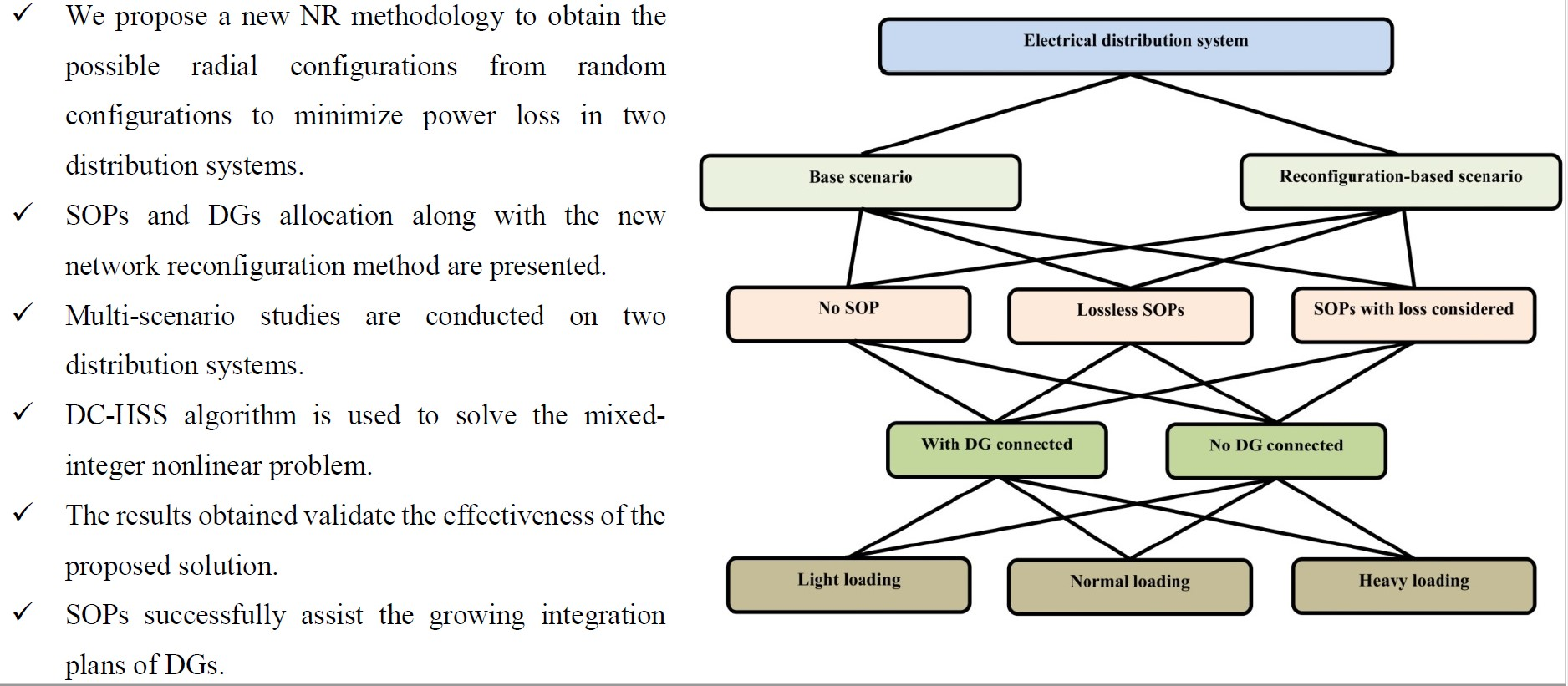
2.2. SOP Modeling

SOPs were first presented in 2011 [38] to provide resilience between distribution feeders. They can be integrated in distribution networks using three topologies, comprising a back-to-back (B2B) voltage source converter (VSC), static series synchronous compensator, and unified power flow controller [39]. In this work, we used a B2B-VSC as the integration topology for SOPs connected to the studied systems because of its flexibility and dynamic capability to enhance the power quality. Figure 1 shows an illustration of SOPs’ integration into a distribution system. To model an SOP, the main equations to perfect the flow of power in the network under study are expressed as follows [16]:

$$P_{i+1}=P_i-P_{i+1}^L-r_{i, i+1}·\frac{P_i^2+Q_i^2}{{\left|V_i\right|}^2}$$

(1)

$$Q_{i+1}=Q_i-Q_{i+1}^L-x_{i, i+1}·\frac{P_i^2+Q_i^2}{{\left|V_i\right|}^2}$$

(2)

$${\left|V_{i+1}\right|}^2={\left|V_i\right|}^2-2\left(r_{i, i+1}·P_i+x_{i,i+1}·Q_i\right)+\left(r_{i, i+1}^2+x_{i,i+1}^2\right)\frac{P_i^2+Q_i^2}{{\left|V_i\right|}^2}$$

(3)

where $P_i$ and $Q_i$ are the injected active and reactive powers at the $i^{th}$ node, $P_{i+1}^L$ and $Q_{i+1}^L$ are the active and reactive powers of the connected loads onto node $i+1$, $\left|V_i\right|$ is the magnitude of the $i^{th}$ node voltage, and $r_{i,i+1}$ and $x_{i,i+1}$ are the feeder resistance and reactance between nodes $i$ and $i+1$.

Then, the SOP is integrated using its active and reactive powers injected at its terminals as presented in Figure 1, in which the summation of the injected powers at the SOP terminals and the internal power loss of its converters must equal zero [16], as expressed in (4). Thus:

$$P_I^{SOP}+P_J^{SOP}+P_I^{SOP-loss}+P_J^{SOP-loss}=0$$

(4)

The reactive power limits [16] are given in (5) and the SOP capacity limit [16] is shown in (6). Thus:

$$Q_I^{SOP-min}\le Q_I^{SOP}\le Q_I^{SOP-max}, \forall I,J\in N_f$$

(5)

$$\sqrt{{\left(P_I^{SOP}\right)}^2+{\left(Q_I^{SOP}\right)}^2}\le S_I^{SOP}, \forall I\in N_f$$

(6)

where $N_f$ is the number of feeders, $P_I^{SOP}$ is the SOP’s active power injected to the $I^{th}$ feeder, $P_J^{SOP}$ is the SOP’s active power to the $J^{th}$ feeder, $P_I^{SOP-loss}$ is the active power loss of the converter connected to the $I^{th}$ feeder, $P_J^{SOP-loss}$ is the internal power loss of the converter connected to the $J^{th}$ feeder, $Q_I^{SOP}$ is the SOP’s reactive power injected to the $I^{th}$ feeder,$Q_J^{SOP}$ is the SOP’s reactive power injected to the $J^{th}$ feeder, $Q_I^{SOP-min}$ and $Q_I^{SOP-max}$ are the minimum and maximum limits of the SOP’s reactive power injected to the $I^{th}$ feeder, and $S_I^{SOP}$ is the maximum capacity limit of the planned SOP. Further, the active loss of each converter ($P_I^{SOP-loss}$ and $P_J^{SOP-loss}$) and the total SOPs active power loss ($P^{SOP-loss}$) are formulated in (7) and (8) as follows [33]:

$$P^{SOP-loss}= {\displaystyle \sum }_{I=1}^{N_f}{P}_I^{SOP- loss}$$

(7)

$$P_I^{SOP-loss}=A_{loss}^{SOP}\sqrt{{\left(P_I^{SOP}\right)}^2+{\left(Q_I^{SOP}\right)}^2}, \forall I\in N_f$$

(8)

where $A_{loss}^{SOP}$ is the loss coefficient of VSCs, which represents leakage in the transferred power to the total power transferred between feeders [33,40,41].

Mathematically, to represent the SOP variables, first, we can consider a lossless SOP, i.e., $P_I^{SOP- loss}=0, \forall I\in N_f;$ hence, a SOP can be represented by its injected active and reactive powers $\left(P_I^{SOP}, Q_I^{SOP}, Q_J^{SOP}\right)$, where $P_J^{SOP}$=$-P_I^{SOP}$. Therefore, multiple SOPs can be modeled by the vector $\left[P_I^{SOP}\left(1\right), Q_I^{SOP}\left(1\right), Q_J^{SOP}\left(1\right), \dots P_M^{SOP}\left(n\right), Q_M^{SOP}\left(n\right), Q_K^{SOP}\left(n\right)\right]$ such that the first three variables in the vector represent the first SOP connected between the Ith and Jth feeders, while the last three variables represent the nth SOP connected between the Mth and Kth feeders.

Second, we can consider the SOP with its losses taken into account, i.e., $P_I^{SOP- loss}\ne 0, \forall I\in N_f;$ hence, starting from (4), we can get $P_I^{SOP- loss}$ as follows:

$$P_J^{SOP}=-P_I^{SOP}-P_I^{SOP- loss}-P_J^{SOP- loss}$$

(9)

Substituting $\left(8\right)$ into $\left(9\right)$:

$$P_J^{SOP}=-P_I^{SOP}-A_{loss}^{SOP}\sqrt{{\left(P_I^{SOP}\right)}^2+{\left(Q_I^{SOP}\right)}^2}-A_{loss}^{SOP}\sqrt{{\left(P_J^{SOP}\right)}^2+{\left(Q_J^{SOP}\right)}^2}$$

(10)

Accordingly, if we set $P_I^{SOP}$,$Q_I^{SOP}$ and $Q_J^{SOP}$ as the SOP’s decision variables, (10) will be a nonlinear equation with one unknown $\left(P_J^{SOP}\right)$. Thus, it can be independently solved using numerical analysis methods such as Newton’s method to find the value of the root ($P_J^{SOP}$) of $\left(10\right)$. Therefore, assuming that $A_{loss}^{SOP}$ is known; an SOP can be represented by its injected active and reactive powers $\left(P_I^{SOP}, Q_I^{SOP}, Q_J^{SOP}\right)$ as the lossless SOP case.

2.3. DG Modeling

In this study, we used two types of DGs. The first includes generators with unity power factor and the second is DGs with smart inverters [21] with a reactive power compensation capability within specified limits of the reactive power.

The DGs with unity PF are limited by the maximum capacity limit $\left(S^{DG}\right)$ of the installed DGs as follows:

$$0\le P_i^{DG}\le S^{DG}$$

(11)

where $P_i^{DG}$ is the active DG power injected at the $i^{th}$ node.

In the second type of DG, the reactive power varies based on specified PF limits, so that $-{\beta }_{min}$ and ${\beta }_{min}$ are the minimum leading and lagging PF values.

$$\sqrt{{\left(P_i^{DG}\right)}^2+{\left(Q_i^{DG}\right)}^2}\le S^{DG}$$

(12)

$$-\tan \left({cos}^{-1}{\beta }_{min}\right)·P_i^{DG}\le Q_i^{DG}\le tan\left({cos}^{-1}{\beta }_{min}\right)·P_i^{DG}$$

(13)

where $Q_i^{DG}$ is the reactive DG power injected at the $i^{th}$ node.

2.4. PQ Indices

In power distribution systems, apart from the functions that describe the objective and constraints that assess the operational performance, there are other indices that evaluate the impacts of the proposed solution on the PQ performance of the studied systems, such as load balancing index ($LBI$), and aggregate voltage deviation index ($AVDI$). The mathematical expressions for these quantities are given as follows:

2.4.1. Load Balancing Index (LBI)

Changing the state of the switches of a distribution system will change its topography. In turn, the loads between the feeders can be distributed to balance the system and avoid the overloading of feeders. In this work, the balancing index ($LBI$) is used to reflect the loading level of each line in the distribution network [16]. The $LBI$ of the $b^{th}$ line is formulated as follows:

$$LB{I}_b={\left(\frac{I_b}{I_b^{rated}}\right)}^2,\forall b\in N_{br}$$

(14)

where $I_b$ is the current flowing in line $b$ and is limited by its rated value $I_b^{rated}$ and $N_{br}$ is the number of lines. Hence, the total load balancing index $LB{I}_{tot}$ is expressed as the sum of the balancing indices of the lines, thus:

$$LB{I}_{tot}={\displaystyle \sum }_{b=1}^{N_{br}}LB{I}_b$$

(15)

$LBI$ of a certain line decreases if the total load connected to this line decreases, and hence, the line current decreases. However, line currents may increase in other lines, increasing their $LBI$s. For that, the $LB{I}_{tot}$ is calculated for all branches to help determine the overall load balancing of all lines in the distribution network.

2.4.2. Aggregate Voltage Deviation Index (AVDI)

Voltage deviation is a measure of the voltage quality in the system. It is formulated as the summation of voltage deviations at all nodes in the system from a reference value of 1 per unit, and is given as:

$$AVDI={\displaystyle \sum }_{i=1}^{N_n}\left|V_i-1\right|$$

(16)

where $i$ and $N_n$ are the node number and total number of nodes, respectively. A system with lower $AVDI$ indicates a secure system with reduced voltage violations.

3. Problem Formulation

3.1. Objective Function

The main aim of this work is to minimize total power loss ($P_{loss}^{tot}$). The objective function $P_{loss}^{tot}$ is divided into two parts, namely the feeder losses due to current flowing in the lines and the SOP’s internal power loss ($P^{SOP-loss}$) as expressed in (17).

$$Min P_{loss}^{tot}={\displaystyle \sum }_{i=1}^{N_n-1}\left(\frac{P_i^2+Q_i^2}{{\left|V_i\right|}^2}· r_{i,i+1}\right)+\mu · P^{SOP-loss}$$

(17)

where $\mu$ = 0 with no SOP losses considered and $\mu$ = 1 if SOP losses are considered.

3.2. Constraints and Operation Conditions

In addition to the radiality requirements described in Section 2. A, power flow equality given in (4), SOP reactive power limits given in (5), SOP capacity limit given in (6), SOP active power loss given in (8), DG capacity limit given in (11) for the first type and (12) for the second type, and DG reactive power limits given in (13), the following constraints regarding voltage magnitudes, lines thermal capacities and the total reactive power injected by DGs and/or SOPs into the system are expressed, respectively, as follows:

$$V_{min}\le \left|V_i\right|\le V_{max }$$

(18)

$$\left|I_{\mathrm{b}}\right|\le I_b^{\mathrm{rated}},\forall b\in N_{br}$$

(19)

$${\displaystyle \sum }_{i=1}^{N_{DG}}{Q}_i^{DG}+{\displaystyle \sum }_{k=1}^{N_{SOP}}\left(Q_I^{SOP}\left(k\right)+Q_J^{SOP}\left(k\right)\right)\le {\displaystyle \sum }_{u=1}^{N_n}{Q}_u^L$$

(20)

where $V_{min}$ and $V_{max}$ represent minimum and maximum voltage limits, respectively, and $N_{DG}$ is the number of connected DGs. It should be noted that the total reactive power injected by DGs and SOPs must not exceed the total demand reactive power, as expressed in (20), to avoid the system’s overcompensation, and to maintain the PF to be within higher lagging values [42,43]. In addition, no reverse power flow is permitted in the system, as expressed in (21). Otherwise, further precautions should be taken by network operators to control excessive reverse power flows and the associated problems resulting from high DG penetration levels.

$$P_i^L-a·P_i^{DG}-b·P_I^{SOP}-c·P_J^{SOP}\ge 0,\forall i\in N_n$$

(21)

where $a$ equals 1 in the case of node $i$ connected to a DG unit, $b$ equals 1 in the case of node $i$ connected to a SOP through feeder $I$, and $c$ equals 1 in the case of node $i$ connected to a SOP through feeder $J$; otherwise, $a=b=c=0$.

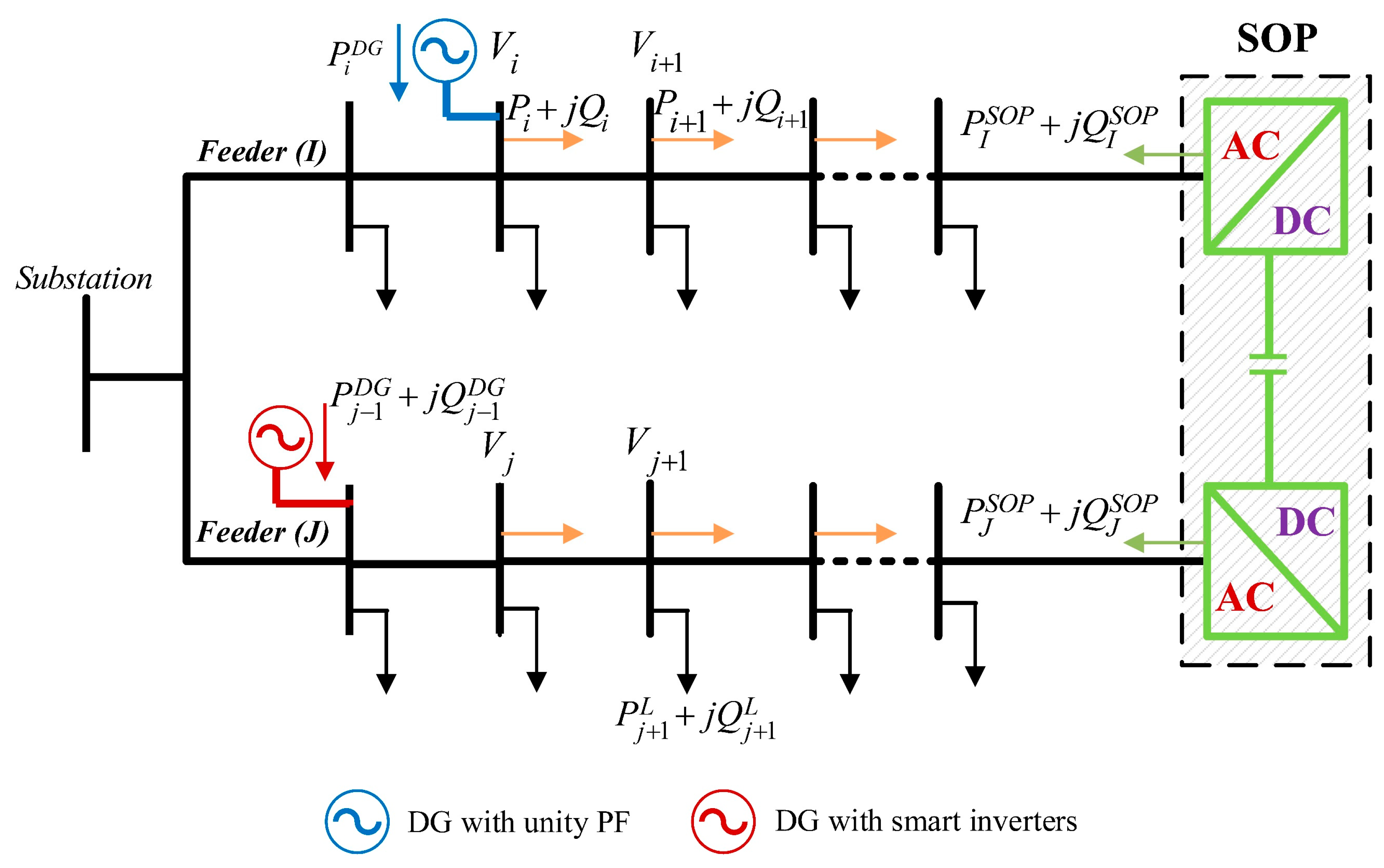
3.3. Search Algorithm

The hyper-spherical search (HSS) algorithm was developed by Karami et al. in 2014 [36] to solve nonlinear functions and was further enhanced in 2016 [37] to consider mixed continuous-discrete decision variables to solve MINLP problems. The DC-HSS has the advantages of fast convergence for optimal/near-optimal solutions and good performance in solving mixed continuous-discrete problems. Therefore, we have used the DC-HSS algorithm to solve our optimization problem.

3.3.1. Continuous HSS

The population is categorized into two types: particles and sphere-centers (SCs). The algorithm searches the inner space of the hyper-sphere to find a new particle position with a better value of objective function as follows:

Step 1: Initialization: the algorithm starts by assigning the population size $\left(N_{pop}\right)$, the distance between the particle, and the sphere-center $\left(r\right),$ taking into account random values between [$r_{min}$, $r_{\max }$], the number of sphere-centers $\left(N_{SC}\right)$, the number of decision variables $\left(N\right)$, the probability of changing the particle’s angle $\left(P{r}_{angle}\right)$, and the maximum number of iterations $\left(Ma{x}_{iter}\right)$. Then, a vector of decision variables $\left(x_i\right)$ is initialized with random values between [$X_i{}_{min}$, $X_i{}_{\max }$] by a uniform probability function. A set equal to $N_{pop}$ containing the objective function values is formed for each vector, in which each vector of the decision variables [$x_1,x_2,\dots , x_N]$ is named as a particle. Further, the particles are sorted according to their objective function values, and then the best $N_{SC}$ particles with the lowest objective function are selected as the initial sphere-centers. The rest of the particles ($N_{pop}-N_{SC})$ are then distributed among the sphere-centers. Finally, a distribution of the ($N_{pop}-N_{SC})$ particles among the SCs is performed by the objective function difference ($OFD$) for each SC, where the $OFD$ is equal to the objective function of SC ($f_{SC}$) subtracted from the maximum objective value of SCs ($OFD=f_{SC}-\underset{SCs}{\max }f$). The normalized dominance for each SC is defined as:

$$D_{SC}=\left|\frac{OF{D}_{SC}}{{{\displaystyle \sum }}_{i=1}^{N_{SC}}OF{D}_i}\right|$$

(22)

A randomly chosen $round\left\{D_{SC}\times \left(N_{pop}-N_{SC}\right)\right\}$ number of particles is assigned to each SC.

Step 2: Searching: each particle seeks to find a better solution by searching the bounding sphere whose center is the assigned SC. The radius of this sphere is $r$. The particle parameters ($r and \theta$) are changed to perform the searching procedure. The angle of the particle is changed by $\propto$, which ranges between $\left(0,2\pi \right)$ with a probability equal to $P{r}_{angle}$. For each particle, $r$ is changed between [$r_{min}$, $r_{\max }$], where $r_{\max }$ can be calculated from (23):

$$r_{\max }=\sqrt{{\displaystyle \sum }_{i=1}^N{\left(x_{i,SC}-x_{i,particle}\right)}^2}$$

(23)

After the search for particles, if a new particle position has a lower objective function value than that of its SC, both the SC and particle will exchange their roles, i.e., the particle becomes the new SC and the old SC becomes the new particle.

Step 3: Dummy particles recovery: An SC with its particles forms a set of particles.

The values of the set objective function ($SOF$) for each set of particles sort these sets to find the worst sets, in which dummy (inactive) particles are located. The $SOF$ is given by (24).

$$SOF=f_{SC}+\left(\gamma ·mean\left\{f_{particles of SC}\right\}\right)$$

(24)

where $\gamma$ is scalar. If $\gamma$ is small, $SOF$ will be biased towards $f_{SC}$, otherwise, $SOF$ will be biased towards $f_{particles of SC}$.

To assign dummy particles to other SCs, two parameters are calculated: the first parameter represents the difference of $SOF$ ($DSOF$) for each set and the second one represents the assigning probability ($AP$) for each SC. These parameters are expressed as follows:

$$DSOF=SOF-\underset{groups}{\max }\left\{SOF of groups\right\}$$

(25)

$$AP=\left[A{P}_1,A{P}_2,\dots \dots ,A{P}_{N_{SC}}\right]$$

(26)

Further, a preset number of particles $N_{newpar}$ with the worst function values are exchanged with the new generated $N_{newpar}$ particles. Hence, after several iterations, the particles and their SCs become close.

Step 4: Termination: the termination criterion is fulfilled if the number of iterations reaches its $Ma{x}_{iter}$ or the difference between the function values of the best SCs is smaller than a pre-set tolerance value.

3.3.2. Discrete HSS

Like the continuous HSS, the discrete HSS starts with the initialization of particles, but with discrete variables. Solutions are then generated randomly from the discrete variables ($X_{id,min},X_{id,min}+1,\dots , X_{id,max}-1,X_{id,max})$ with a uniform probability. $N_{SC}$ particles with the lowest function values are assigned as SCs. The rest of the particles are distributed among the SCs. Then, the same searching procedure as the continuous HSS is performed. It should be mentioned that the angle $\propto$ is not considered in the searching procedure of the discrete HSS and the only parameter used is the radius $r_d$, where $r_d$ is selected between ($r_{d,min},r_{d,min}+1,\dots , r_{d,max}-1,r_{d,max})$. $r_{d,max}$ is calculated as follows:

$$r_{d,max}=\sqrt{{\displaystyle \sum }_{i=1}^N{\left(x_{i_d,SC}-x_{i_d,particle}\right)}^2}$$

(27)

The other steps will be performed as presented in the continuous HSS algorithm.

3.3.3. Discrete-continuous HSS (DC-HSS)

DC-HSS combines both continuous and discrete HSS algorithms, in which the particles contain both continuous and discrete variables. The procedure for the continuous variables is structured as presented in the continuous HSS formulation, whilst the procedure for the discrete variables is structured as presented in the discrete HSS formulation. To sum up, the optimization parameters of DC-HSS are as follows: $N_{pop}$=1000,$N_{SC}=100$, $r_{min}=0$, $r_{\max }=1$, $r_{d,min}=0$, $r_{d,max}=1$, $N_{newpar}=5$, $P{r}_{angle}=75\%$, and $Ma{x}_{iter}=1000$. Figure 2 illustrates a comprehensive flowchart for the proposed problem formulation using the DC-HSS algorithm.

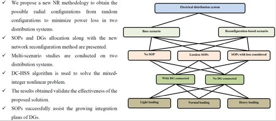
4. Results and Discussion

In this section, the results obtained in the nine scenarios are presented for the IEEE 33-node and 83-node systems under different loading conditions. Further, the contribution of SOP loss to the total active power loss as well as the effect of increasing the number of SOPs connected to the systems are studied. Case studies are carried out on an Intel Core i7 CPU, second generation, at 2.2 GHz and 3 GHz maximum turbo boost speed, with 6 GB of RAM with speed 1333 MHz, 6 MB cache memory and contains SSD hard disk at 550 MB per second.

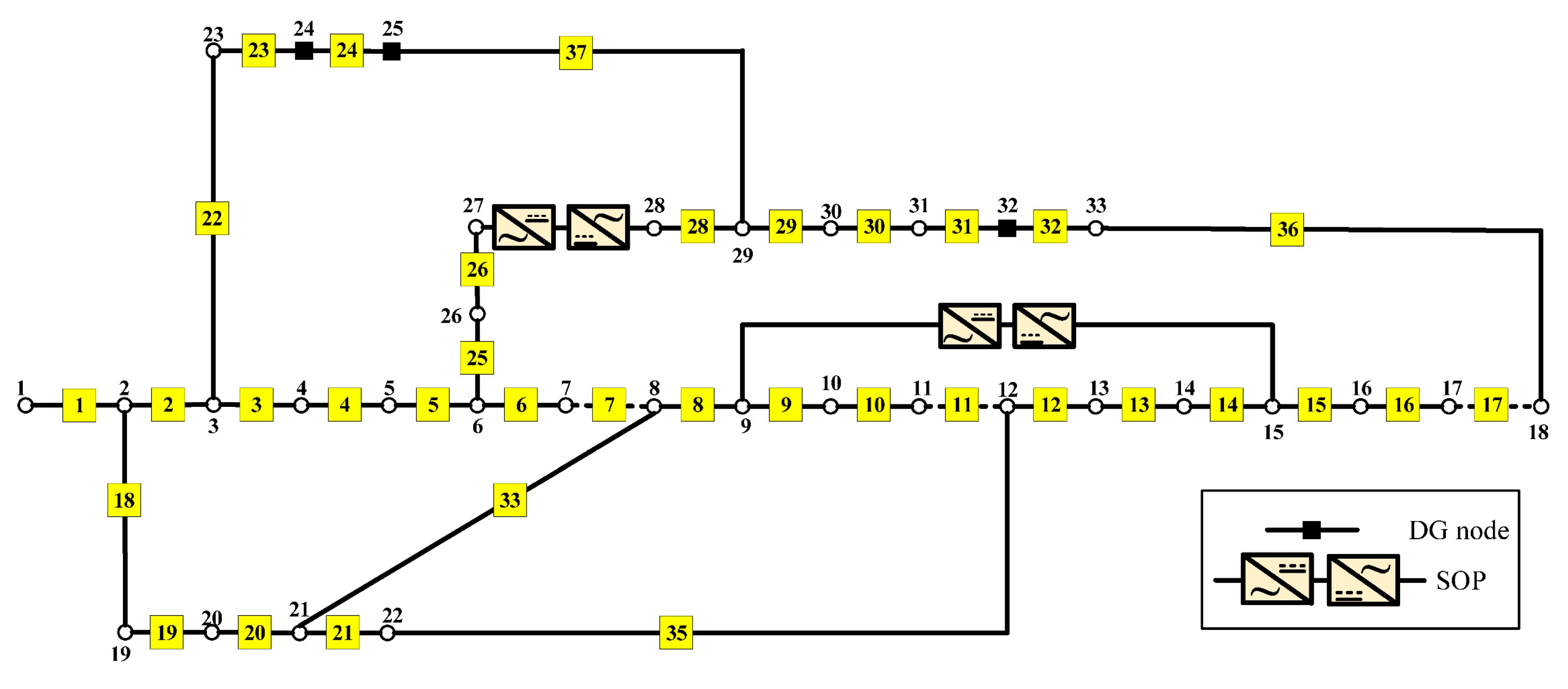
4.1. IEEE 33-Node Distribution System

The IEEE 33-node base configuration consists of 32 sectionalized lines and 5 tie-lines as shown in Figure 3. The number of SOPs that can be installed ranges from 1 to 5, i.e., $N_{SOP}\in \left[1,5\right]$, where the individual SOP rating ($S_I^{SOP}=S_J^{SOP}$) is 1 MVA and $A_{loss}^{SOP}$ equals 0.02 [33,40,41]. $N_{DG}$ is set to 3, while $S^{DG}$ equals 1 MVA with unity PF. $V_{min }$ and $V_{max}$ values are 0.95 and 1.05 p.u., respectively. Also, $I_b^{\mathrm{rated}}$ is set to 300 A.

First, the results obtained for the system in the first three scenarios with no SOPs installed are given in

Table 2. Total power losses and PQ indices for scenarios 1, 2 and 3: IEEE 33-node system.

Loading Level	Scenario	${\mathit{P}}_{\mathit{l}\mathit{o}\mathit{s}\mathit{s}}^{\mathit{t}\mathit{o}\mathit{t}} \left(\mathbf{kW}\right)$	$\mathit{L}\mathit{B}{\mathit{I}}_{\mathit{t}\mathit{o}\mathit{t}}$	$\mathit{A}\mathit{V}\mathit{D}\mathit{I}$
Light (50%)	1	33.646	0.058	0.678
	2	41.212	0.376	0.862
	3	21.346	0.178	0.500
Normal (100%)	1	NA
	2
	3	90.013	0.765	1.064
Heavy (160%)	1	NA
	2
	3

.

On the one hand, the results clarify that optimizing the NR and DGs allocation strategies separately cannot satisfy the voltage requirements in either the normal or heavy loading conditions, and only a sub-optimal performance can be achieved in the light loading case. On the other hand, simultaneous NR and DGs allocation can meet the problem limits in light and normal loading conditions only. Hence, one can conclude that the first three scenarios cannot guarantee acceptable performance level of the IEEE 33-node system with loads alteration.

Second, the results obtained for Scenarios 4 to 9 with lossless SOPs installed in the system are presented in

Table 3. Total Power Losses and PQ Indices for Scenarios 4 to 9 with Lossless SOPs Installed: IEEE 33-node system.

Scenario	${\mathit{N}}_{\mathit{S}\mathit{O}\mathit{P}}$	Light Loading (50%)			Normal Loading (100%)			Heavy Loading (160%)
		${\mathit{P}}_{\mathit{l}\mathit{o}\mathit{s}\mathit{s}}^{\mathit{t}\mathit{o}\mathit{t}} \left(\mathbf{kW}\right)$	$\mathit{L}\mathit{B}{\mathit{I}}_{\mathit{t}\mathit{o}\mathit{t}}$	$\mathit{A}\mathit{V}\mathit{D}\mathit{I}$	${\mathit{P}}_{\mathit{l}\mathit{o}\mathit{s}\mathit{s}}^{\mathit{t}\mathit{o}\mathit{t}} \left(\mathbf{kW}\right)$	$\mathit{L}\mathit{B}{\mathit{I}}_{\mathit{t}\mathit{o}\mathit{t}}$	$\mathit{A}\mathit{V}\mathit{D}\mathit{I}$	${\mathit{P}}_{\mathit{l}\mathit{o}\mathit{s}\mathit{s}}^{\mathit{t}\mathit{o}\mathit{t}} \left(\mathbf{kW}\right)$	$\mathit{L}\mathit{B}{\mathit{I}}_{\mathit{t}\mathit{o}\mathit{t}}$	$\mathit{A}\mathit{V}\mathit{D}\mathit{I}$
4	1	38.723	0.343	0.745	NA			NA
	2	33.686	0.303	0.709
	3	32.097	0.292	0.701	144.337	1.285	1.085
	4	29.481	0.271	0.603	143.107	1.255	0.973
	5	27.420	0.252	0.572	128.576	1.145	1.093
5	1	23.936	0.211	0.565	NA			NA
	2	22.323	0.199	0.427	91.206	0.823	0.928
	3	22.613	0.204	0.444	93.576	0.842	0.969
	4	22.028	0.205	0.413	89.932	0.833	0.877	269.511	2.317	0.977
	5	22.323	0.209	0.403	89.942	0.832	0.830	267.975	2.275	1.081
6	1	23.709	0.215	0.536	98.803	0.897	1.126	NA
	2	22.689	0.202	0.464	90.777	0.824	0.931
	3	23.384	0.213	0.502	90.303	0.839	0.914	254.480	2.228	1.281
	4	22.586	0.205	0.443	89.092	0.823	0.882	255.053	2.255	1.239
	5	23.961	0.204	0.399	89.429	0.853	0.848	258.36	2.220	1.141
7	1	20.548	0.179	0.583	NA			NA
	2	20.548	0.179	0.583
	3	19.796	0.175	0.524	87.745	0.759	1.142
	4	19.454	0.172	0.546	77.212	0.681	1.076
	5	17.884	0.162	0.512	73.512	0.670	1.050
8	1	15.299	0.121	0.495	NA			NA
	2	13.760	0.114	0.428	55.498	0.461	0.822	153.348	1.262	1.261
	3	13.674	0.114	0.443	54.750	0.464	0.785	142.402	1.217	1.221
	4	14.503	0.123	0.416	56.238	0.482	0.798	166.628	1.478	1.302
	5	14.565	0.129	0.387	52.306	0.456	0.764	170.249	1.358	1.141
9	1	14.269	0.122	0.433	57.851	0.508	0.752	160.812	1.412	1.303
	2	13.840	0.118	0.373	51.748	0.445	0.742	144.826	1.265	1.165
	3	13.295	0.116	0.359	49.954	0.448	0.653	125.768	1.133	1.066
	4	11.869	0.110	0.312	50.176	0.444	0.634	137.325	1.241	1.091
	5	12.087	0.106	0.353	45.885	0.433	0.601	122.062	1.131	1.034

under the three loading conditions.

On the one hand, the results obtained with one SOP installed in the system with or without NR in the case of no DGs connected exhibit poor performance, which can be explained by the lack of an acceptable solution to the problem because of minimum voltage value violation under both the normal and heavy loading conditions, as shown in Scenarios 4 and 5. Therefore, to meet the minimum voltage requirement, the reactive power should be compensated by installing additional SOPs, as presented in Scenario 6, with 3 to 5 SOPs when NR was considered. On the other hand, the results obtained when DGs were connected into the system without NR (Scenario 7) decreased the need for an increasing number of installed SOPs. Further, when NR is enabled, an additional reduction of the number of SOPs is noticed, which will result in reducing the power losses, as revealed by the proposed Scenario 9 because it allows freedom in locating SOPs.

To sum up, the results obtained for Scenario 9 (simultaneous NR with DGs and SOPs allocation) resulted in the best solutions, highlighted in bold in Table 3, with 5 SOPs at the normal and heavy loading levels and 4 SOPs at the light loading level compared to the results obtained by the other scenarios, in which the power losses are reduced by 74.787% at normal, 77.362% at light, and 78.788% at heavy loading levels with respect to the corresponding base system values. Also, the improvement of the voltage profile obtained in Scenario 9 for the system at the normal loading condition is shown in Figure 4.

Thirdly, the results obtained for Scenarios 4 to 9 with the SOPs’ internal power losses considered are presented in

Table 4. Total Power Losses and PQ Indices for Scenarios 4 to 9 with SOP Losses Considered: IEEE 33-node system.

Scenario	${\mathit{N}}_{\mathit{S}\mathit{O}\mathit{P}}$	Light Loading (50%)			Normal Loading (100%)			Heavy Loading (160%)
		${\mathit{P}}_{\mathit{l}\mathit{o}\mathit{s}\mathit{s}}^{\mathit{t}\mathit{o}\mathit{t}} \left(\mathbf{kW}\right)$	$\mathit{L}\mathit{B}{\mathit{I}}_{\mathit{t}\mathit{o}\mathit{t}}$	$\mathit{A}\mathit{V}\mathit{D}\mathit{I}$	${\mathit{P}}_{\mathit{l}\mathit{o}\mathit{s}\mathit{s}}^{\mathit{t}\mathit{o}\mathit{t}} \left(\mathbf{kW}\right)$	$\mathit{L}\mathit{B}{\mathit{I}}_{\mathit{t}\mathit{o}\mathit{t}}$	$\mathit{A}\mathit{V}\mathit{D}\mathit{I}$	${\mathit{P}}_{\mathit{l}\mathit{o}\mathit{s}\mathit{s}}^{\mathit{t}\mathit{o}\mathit{t}} \left(\mathbf{kW}\right)$	$\mathit{L}\mathit{B}{\mathit{I}}_{\mathit{t}\mathit{o}\mathit{t}}$	$\mathit{A}\mathit{V}\mathit{D}\mathit{I}$
4	1	45.414	0.376	0.859	NA			NA
	2	45.796	0.361	0.819
	3	35.479	0.292	0.699	177.087	1.099	1.042
	4	35.083	0.281	0.641	133.125	1.057	1.194
	5	39.932	0.289	0.635	162.892	1.093	1.049
5	1	27.184	0.219	0.572	NA			NA
	2	27.185	0.219	0.573	110.805	0.925	1.147
	3	30.747	0.209	0.533	113.375	0.887	1.100
	4	37.655	0.221	0.445	126.837	0.964	0.887	415.433	2.497	0.811
	5	38.209	0.282	0.537	165.753	0.938	1.047	461.002	2.689	0.751
6	1	26.753	0.212	0.526	106.317	0.921	1.125	NA
	2	26.753	0.212	0.526	104.076	0.881	1.015
	3	26.754	0.212	0.525	104.774	0.858	0.934	427.952	2.525	1.283
	4	26.824	0.205	0.456	106.070	0.897	1.060	386.968	2.338	1.216
	5	29.629	0.220	0.544	119.559	0.915	1.058	377.700	2.295	1.166
7	1	23.883	0.188	0.592	NA			NA
	2	27.727	0.201	0.659
	3	27.669	0.209	0.609
	4	29.336	0.213	0.632
	5	36.100	0.234	0.579	114.118	0.783	1.123
8	1	18.489	0.129	0.502	NA			NA
	2	18.489	0.129	0.501	68.064	0.509	0.899	204.716	1.131	1.239
	3	19.670	0.118	0.417	72.782	0.494	0.853	196.995	1.279	1.249
	4	29.082	0.129	0.385	86.147	0.508	0.966	317.274	1.712	1.309
	5	25.052	0.129	0.336	94.222	0.578	0.769	220.982	1.289	1.189
9	1	16.828	0.126	0.441	67.019	0.525	0.911	NA
	2	16.575	0.119	0.375	66.131	0.527	0.804	193.316	1.362	1.322
	3	17.144	0.126	0.446	73.735	0.483	0.782	189.168	1.352	1.238
	4	20.329	0.127	0.390	74.077	0.500	0.746	193.753	1.211	1.029
	5	19.819	0.118	0.408	74.695	0.469	0.602	188.831	1.176	1.135

at the three loading levels.

Regardless of economic aspects, in the lossless SOP scenarios, the system with an increased number of installed SOPs becomes more efficient because of the considerable power loss reduction. However, this is not the case if the SOPs’ internal losses are considered, because power loss minimization is considerably affected by the SOPs internal losses. This makes clear that loss minimization is not guaranteed by installing more SOPs. In addition, one cannot simply suppose that increasing the number of installed SOPs will increase the SOPs’ internal losses proportionally, as this depends on the power transferred by the SOPs and also on the SOPs’ locations, as clarified in Figure 5, with results obtained in Scenario 9 that make clear that choosing an appropriate number of SOPs is a matter of optimization. Moreover, after considering the internal power losses of the SOPs, it is obvious that the results obtained for Scenario 9 are the best results obtained so far compared to the results obtained for the other scenarios, in which the power losses are reduced by 67.374% using two SOPs at normal, 64.374% using two SOPs at light, and 67.184% using five SOPs at heavy loading levels. All values are given with respect to the corresponding base system values. Furthermore, all the considered PQ indices are enhanced using the same scenario by different values as presented in Table 4, which validates the effectiveness of the proposed solution. The improvement of the voltage profile obtained in Scenario 9 for the system at the normal loading condition with the SOPs’ power loss considered is shown in Figure 6. A detailed summary of the optimal results obtained for scenarios 4 to 9 at the normal loading condition is given in

Table A1. Optimal system configuration, sizing, and locations of SOPs and DGs for scenarios 4 to 9 without SOPs internal losses at normal loading level: IEEE 33-node distribution system.

Scenario	Tie-Lines	SOPs Locations (lines)	SOPs Sizing			DG Node	DG Sizing (MW)
			$$\begin{gathered} {\mathit{P}}_{\mathit{I}}^{\mathit{S}\mathit{O}\mathit{P}} \\ \left(\mathbf{MW}\right) \end{gathered}$$	$$\begin{gathered} {\mathit{Q}}_{\mathit{I}}^{\mathit{S}\mathit{O}\mathit{P}} \\ \left(\mathbf{MVAr}\right) \end{gathered}$$	$$\begin{gathered} {\mathit{Q}}_{\mathit{J}}^{\mathit{S}\mathit{O}\mathit{P}} \\ \left(\mathbf{MVAr}\right) \end{gathered}$$
4	-	33	0.2000	0.0818	0	NA
		34	0	0	0.0933
		35	0.0600	0.2432	0.6847
		36	0.0900	0.0344	0.5634
		37	0	0	0
5	7	11	0.0450	0.0263	0.0171	NA
		14	−0.0600	0.2924	0.0117
		32	−0.0600	0.3360	0.1729
		37	−0.1200	0.2272	0.6886
6	7	11	0.0450	0	0	NA
		14	0	0	0.0920
		32	−0.0600	0.3123	0.0885
		37	−0.1200	0.3670	0.6980
7	-	33	0	0	0.088	24	0.4200
		34	0	0	0
		35	0.06	0	0	25	0.4200
		36	0.09	0	0	32	0.2100
		37	−0.0913	0.394984	0.521994
8	-	7	−0.0131	0	0.173922	24	0.4200
		11	0.045	0	0
		14	−0.06	0.071586	0	25	0.4200
		32	−0.06	0.366156	0.196486	32	0.2100
		37	−0.12	0.28405	0.521668
9	-	7	−0.2	0.126	0.06107	24	0.4200
		11	−0.06	0	0
		28	−0.12	0	0.812957	25	0.4200
		34	−0.06	0.036864	0.077424	32	0.2100
		36	0.09	0.286571	0.239091

and

Table A2. Optimal system configuration, sizing, and locations of SOPs and DGs for scenarios 4 to 9 with SOPs internal losses considered at normal loading level: IEEE 33-node distribution system.

Scenario	Tie-lines	SOPs Locations (lines)	SOPs Sizing			DG Node	DG Sizing (MW)
			$$\begin{gathered} {\mathit{P}}_{\mathit{I}}^{\mathit{S}\mathit{O}\mathit{P}} \\ \left(\mathbf{MW}\right) \end{gathered}$$	$$\begin{gathered} {\mathit{Q}}_{\mathit{I}}^{\mathit{S}\mathit{O}\mathit{P}} \\ \left(\mathbf{MVAr}\right) \end{gathered}$$	$$\begin{gathered} {\mathit{Q}}_{\mathit{J}}^{\mathit{S}\mathit{O}\mathit{P}} \\ \left(\mathbf{MVAr}\right) \end{gathered}$$
4	36	33	0.2000	0.0333	0.0538	NA
		34	−0.0652	0.0066	0.3065
		35	0.0600	0.1494	0.0480
		37	−0.1252	0	0
5	7-11-32	14	0	0	0.1582	NA
		37	−0.1261	0.0918	0.0138
6	7-11-32	14	−0.0628	0.0315	0.2978	NA
		37	−0.1249	0.0009	0.8776
7	-	33	0	0	0.082994	24	0.4200
		34	−0.06245	0	0.120284
		35	0.06	0	0	25	0.4200
		36	0.09	0	0	32	0.2100
		37	−0.12568	0.071358	0.166987
8	7-11-14	32	−0.0624	0	0.1901	24	0.4200
						25	0.4200
		37	−0.1260	0.0853	0.3983	32	0.2100
9	7-11-17	27	−0.0624	0.000293	0.6938	24	0.4200
		34	−0.0626	0.0243	0.2831	25	0.4200
						32	0.2100

in the Appendix A. Also, the IEEE 33-node system after applying Scenario 9 in a normal loading condition is shown in Figure A1 in Appendix A. Finally, optimizing the NR, DGs, and SOPs allocation strategies collectively facilitates collaboration between strategies, which will help achieve the best performance level of the system.

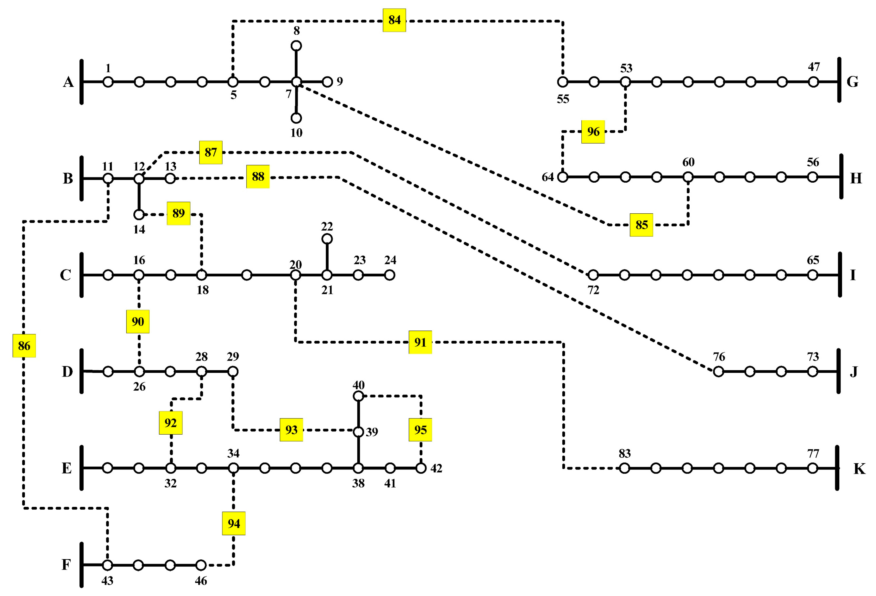
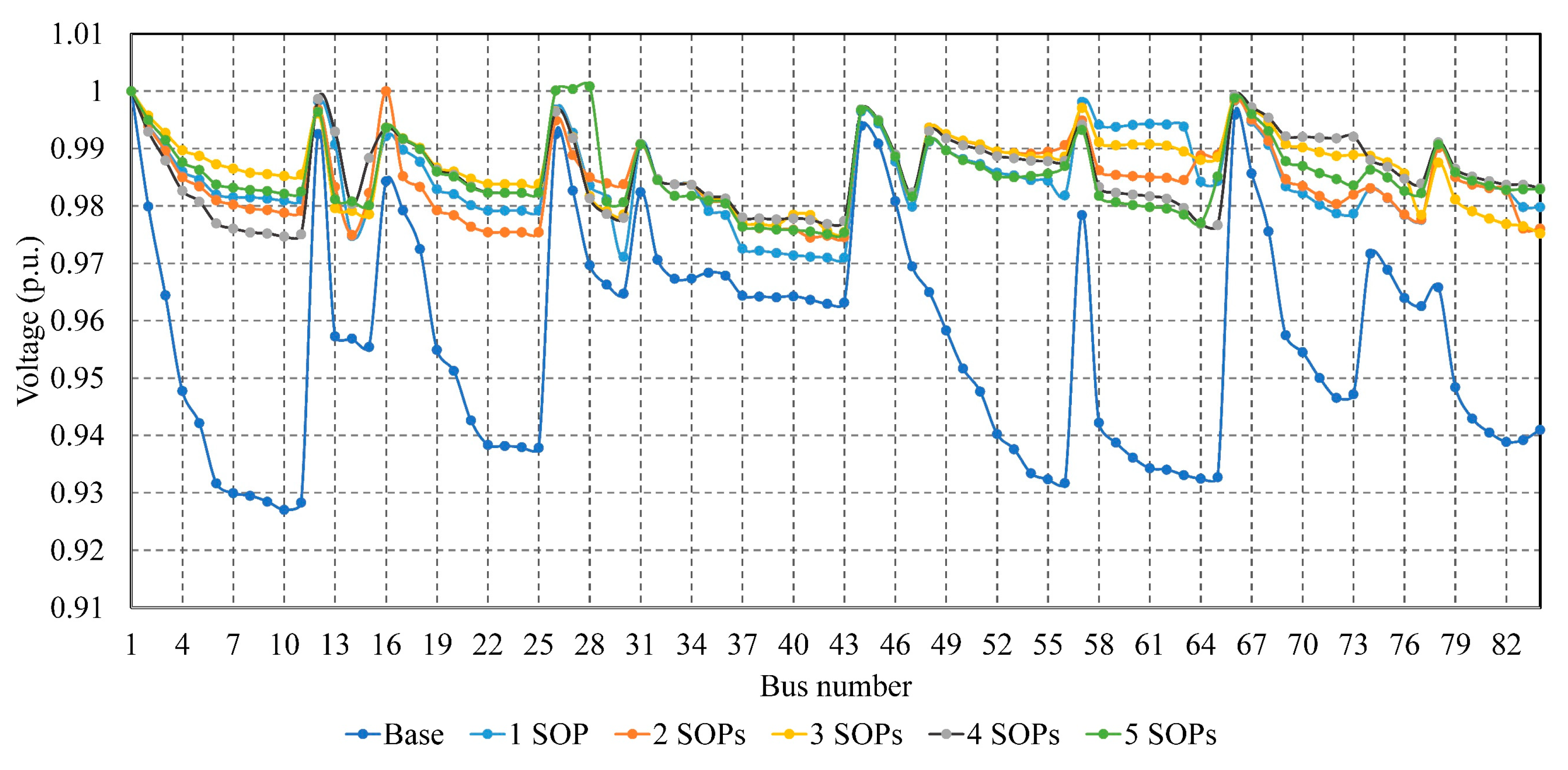
4.2. 83-node Distribution System

In order to validate the effectiveness of Scenario 9 proposed in this work, it was examined on an 83-node balanced distribution system from a power company in Taiwan, in which the 83-node base configuration consisted of 83 sectionalized lines and 13 tie-lines, as shown in Figure 7. The number of SOPs that can be installed ranges from 1 to 5, i.e., $N_{SOP}\in \left[1,5\right]$, where the individual SOP rating ($S_I^{SOP}=S_J^{SOP}$) is 1.5 MVA and $A_{loss}^{SOP}$ equals 0.02 [33,40,41]. $N_{DG}$ is set to 8 with $S^{DG}$ equal to 3 MVA and PF ranges from 0.95 lagging to unity. The $V_{min}$ and $V_{max}$ values are 0.95 and 1.05 p.u., respectively. Also, $I_b^{\mathrm{rated}}$ is set to 310 A.

First, the results obtained for the system in the first three scenarios with no SOPs installed in the system are given in

Table 5. Total power losses and PQ indices for scenarios 1, 2 and 3: 83-node system.

Loading Level	Scenario	${\mathit{P}}_{\mathit{l}\mathit{o}\mathit{s}\mathit{s}}^{\mathit{t}\mathit{o}\mathit{t}} \left(\mathbf{kW}\right)$	$\mathit{L}\mathit{B}{\mathit{I}}_{\mathit{t}\mathit{o}\mathit{t}}$	$\mathit{A}\mathit{V}\mathit{D}\mathit{I}$
Light (50%)	1	113.382	3.237	1.303
	2	97.496	2.713	1.249
	3	87.033	2.425	1.128
Normal (100%)	1	470.241	13.259	2.654
	2	NA
	3	368.364	10.699	2.309
Heavy (130%)	1	NA
	2
	3

. Once more, the results make it clear that optimizing the NR and DGs allocation strategies separately cannot satisfy the voltage requirements at the heavy loading level, and only a sub-optimal performance can be achieved at the light and normal loading levels. However, simultaneous NR and DGs allocation can meet the problem limits considered in the normal and light loading conditions only. Second, the results obtained for Scenarios 4 to 9 with/without SOPs internal losses in the system are presented in

Table 6. Total power losses and PQ indices for scenarios 4 to 9 without SOP losses: 83-node system.

Scenario	${\mathit{N}}_{\mathit{S}\mathit{O}\mathit{P}}$	Light Loading (50%)			Normal Loading (100%)			Heavy Loading (130%)
		${\mathit{P}}_{\mathit{l}\mathit{o}\mathit{s}\mathit{s}}^{\mathit{t}\mathit{o}\mathit{t}} \left(\mathbf{kW}\right)$	$\mathit{L}\mathit{B}{\mathit{I}}_{\mathit{t}\mathit{o}\mathit{t}}$	$\mathit{A}\mathit{V}\mathit{D}\mathit{I}$	${\mathit{P}}_{\mathit{l}\mathit{o}\mathit{s}\mathit{s}}^{\mathit{t}\mathit{o}\mathit{t}} \left(\mathbf{kW}\right)$	$\mathit{L}\mathit{B}{\mathit{I}}_{\mathit{t}\mathit{o}\mathit{t}}$	$\mathit{A}\mathit{V}\mathit{D}\mathit{I}$	${\mathit{P}}_{\mathit{l}\mathit{o}\mathit{s}\mathit{s}}^{\mathit{t}\mathit{o}\mathit{t}} \left(\mathbf{kW}\right)$	$\mathit{L}\mathit{B}{\mathit{I}}_{\mathit{t}\mathit{o}\mathit{t}}$	$\mathit{A}\mathit{V}\mathit{D}\mathit{I}$
4	1	112.236	3.035	1.163	NA			NA
	2	107.777	2.929	0.976
	3	106.452	2.911	0.847
	4	98.345	2.662	0.958
	5	99.079	2.697	0.779
5	1	106.662	3.000	1.213	441.694	12.273	2.501
	2	103.194	2.898	1.137	427.829	12.010	2.373
	3	104.861	2.945	1.029	421.891	11.660	2.297
	4	101.766	2.773	1.062	412.534	11.248	2.171
	5	96.026	2.769	0.811	390.587	11.017	1.893
6	1	105.558	3.014	1.034	442.042	12.584	2.293
	2	100.563	2.878	0.969	425.271	12.106	2.229
	3	96.450	2.747	0.823	405.221	11.232	2.137
	4	92.742	2.661	0.825	385.354	10.501	1.836
	5	89.949	2.484	0.696	407.074	10.428	2.109
7	1	54.413	1.511	0.895	231.704	6.396	1.879	439.890	12.036	2.773
	2	54.935	1.511	0.887	226.485	6.284	1.614	387.021	10.649	2.325
	3	52.594	1.496	0.680	214.617	6.000	1.668	394.187	10.901	2.233
	4	49.215	1.382	0.688	192.775	5.519	1.464	371.243	10.239	2.214
	5	52.882	1.512	0.632	197.090	5.579	1.562	333.774	9.363	1.816
8	1	60.405	1.797	1.019	253.559	7.358	2.019	NA
	2	58.648	1.755	0.928	240.294	7.059	1.925
	3	62.326	1.822	0.899	249.926	7.224	1.979
	4	57.268	1.679	0.879	243.006	6.816	1.795
	5	54.513	1.681	0.723	210.822	6.284	1.584
9	1	51.425	1.456	0.792	219.131	6.282	1.713	379.446	10.806	2.345
	2	49.481	1.382	0.667	203.24	5.821	1.550	345.422	10.022	1.997
	3	46.868	1.321	0.641	192.115	5.392	1.463	348.556	9.905	2.196
	4	43.469	1.238	0.587	189.128	5.084	1.379	345.018	10.815	2.080
	5	45.122	1.309	0.566	189.073	5.140	1.386	302.561	9.163	1.571

and

Table 7. Total power losses and PQ indices for scenarios 4 to 9 with SOP losses considered: 83-node system.

Scenario	${\mathit{N}}_{\mathit{S}\mathit{O}\mathit{P}}$	Light Loading (50%)			Normal Loading (100%)			Heavy Loading (130%)
		${\mathit{P}}_{\mathit{l}\mathit{o}\mathit{s}\mathit{s}}^{\mathit{t}\mathit{o}\mathit{t}} \left(\mathbf{kW}\right)$	$\mathit{L}\mathit{B}{\mathit{I}}_{\mathit{t}\mathit{o}\mathit{t}}$	$\mathit{A}\mathit{V}\mathit{D}\mathit{I}$	${\mathit{P}}_{\mathit{l}\mathit{o}\mathit{s}\mathit{s}}^{\mathit{t}\mathit{o}\mathit{t}} \left(\mathbf{kW}\right)$	$\mathit{L}\mathit{B}{\mathit{I}}_{\mathit{t}\mathit{o}\mathit{t}}$	$\mathit{A}\mathit{V}\mathit{D}\mathit{I}$	${\mathit{P}}_{\mathit{l}\mathit{o}\mathit{s}\mathit{s}}^{\mathit{t}\mathit{o}\mathit{t}} \left(\mathbf{kW}\right)$	$\mathit{L}\mathit{B}{\mathit{I}}_{\mathit{t}\mathit{o}\mathit{t}}$	$\mathit{A}\mathit{V}\mathit{D}\mathit{I}$
4	1	126.023	3.313	1.349	NA			NA
	2	134.346	3.219	1.060
	3	139.039	3.364	1.201
	4	144.968	3.049	1.279
	5	145.084	2.893	1.090
5	1	117.084	3.250	1.287	473.623	12.788	2.610
	2	119.178	3.170	1.267	478.019	12.783	2.568
	3	133.988	3.187	1.227	491.723	12.480	2.504
	4	142.552	2.934	1.188	512.955	12.595	2.374
	5	145.349	3.024	1.156	518.085	11.919	2.181
6	1	114.048	3.263	1.278	472.069	13.065	2.646
	2	116.980	3.218	1.254	470.112	12.527	2.539
	3	122.259	3.117	1.157	469.115	12.495	2.513
	4	119.642	3.049	1.163	497.125	12.839	2.593
	5	116.877	2.939	1.158	502.876	11.627	2.284
7	1	65.706	1.787	1.078	271.560	6.292	1.969
	2	81.718	1.531	0.822	286.725	6.845	1.868
	3	105.414	1.595	0.742	308.381	7.518	1.889
	4	100.211	1.451	0.719	317.376	5.966	1.637
	5	115.202	1.432	0.696	343.568	5.853	1.574
8	1	66.890	1.827	1.039	271.865	7.287	2.058
	2	77.613	1.909	1.048	310.045	7.159	1.977
	3	90.195	1.914	1.002	343.867	7.744	2.030
	4	122.116	1.906	0.972	348.229	7.929	2.073
	5	154.082	1.918	0.825	344.441	6.647	1.716
9	1	67.280	1.764	1.043	253.076	6.244	1.836	436.212	11.325	2.654
	2	76.316	1.718	0.888	255.124	6.227	1.836	443.586	10.939	2.389
	3	95.475	1.693	0.942	272.452	5.754	1.737	464.298	11.017	2.451
	4	127.245	1.529	0.924	287.265	5.949	1.758	517.269	11.613	2.551
	5	96.895	1.847	0.976	284.899	6.240	1.619	509.753	10.066	2.306

at the three loading levels.

From Table 6 and Table 7, it can be observed that installing SOPs without NR optimization and DGs allocation (Scenario 4) failed to operate the system within the specified limits, even after increasing the number of SOPs. On the one hand, for the lossless SOPs cases, Scenario 7 succeeded in finding acceptable solutions for the problem, contrary to Scenarios 4, 5, 6, and 8, all of which failed to find an acceptable solution, even with an increased number of SOPs. On the other hand, taking SOPs’ losses into account, Scenarios 4 to 8 were not capable of finding an acceptable solution for the problem at a heavy loading level. Still, Scenario 9 remains the most successful scenario as it has the ability to improve the system performance and keep it within the specified limits.

The improvement of the voltage profile obtained in Scenario 9 for the system at the normal loading condition with SOPs power loss considered is shown in Figure 8. The contribution of SOPs’ losses to the total power losses with different numbers of SOPs is clarified in Figure 9, where the contour plots agree with the conclusions drawn in the IEEE 33-node case study. A detailed summary of the optimal results obtained in Scenarios 5 to 9 at the normal loading condition is given in

Table A3. Optimal system configuration, sizing and locations of SOPs and DGs for scenarios 5 to 9 without SOPs internal losses at normal loading level: 83-node distribution System.

Scenario	Tie-Lines	SOPs Locations (lines)	SOPs Sizing			DG Node	DG Sizing (MVA)	PF
			$$\begin{gathered} {\mathit{P}}_{\mathit{I}}^{\mathit{S}\mathit{O}\mathit{P}} \\ \left(\mathbf{MW}\right) \end{gathered}$$	$$\begin{gathered} {\mathit{Q}}_{\mathit{I}}^{\mathit{S}\mathit{O}\mathit{P}} \\ \left(\mathbf{MVAr}\right) \end{gathered}$$	$$\begin{gathered} {\mathit{Q}}_{\mathit{J}}^{\mathit{S}\mathit{O}\mathit{P}} \\ \left(\mathbf{MVAr}\right) \end{gathered}$$
5	13-34-39-55-63-83-86-89	7	−0.4	1.5	0.9757	NA
		42	0.2	0.4398	0.4719
		72	0.4184	1.4214	1.3143
		90	0.3	0.1856	0.5016
		92	0.7229	0.3661	1.1009
6	13-34-39-42-84-86-89-90-96	72	1.1439	0.3959	1.4468
		82	−0.1	1.1822	0.3869
		85	0.4	1.4312	0.6977
		92	−0.2	1.4781	0.6503
7	84-86-88-89-90-91-94-95-96	85	0.1547	1.492	0.8203	6	1.100	0.9658
						12	1.200	0.9500
		87	0.2941	1.0794	0.7539	19	1.200	0.9500
						28	1.547	0.9817
		92	−0.2	0.9864	1.0761	31	1.799	0.9502
						71	2.000	0.9500
		93	0.2	0.4686	0.6413	75	1.200	0.9500
						79	2.000	0.9500
8	13-34-39-55-63-83-86-89	7	−0.4	0.5959	0.7569	6	1.100	0.9747
		42	0.200	0.4948	0.5371	12	0.995	0.9503
						19	1.200	0.9535
		72	0.3509	0.8314	0.3136	28	1.800	0.9501
						31	1.800	0.9501
		90	−0.1	1.2025	1.1796	71	1.274	0.9501
						75	1.200	0.9502
		92	−0.200	0.350	1.3027	79	2.000	0.9501
9	7-13-16-32-34-72-86-95	38	−0.02	0.239	0.493	6	1.100	0.9509
		55	0.500	1.399	0.804	12	1.200	0.9502
						19	1.200	0.9500
		64	0.300	0.9497	0.576	28	1.782	0.9500
						31	1.678	0.9501
		89	−0.091	0.764	1.236	71	2.000	0.9500
						75	1.200	0.9500
		91	0.300	0.8106	1.033	79	2.000	0.9500

and

Table A4. Optimal system configuration, sizing, and locations of SOPs and DGs for scenarios 5 to 9 with SOPs internal losses considered at normal loading level: 83-node distribution system.

Scenario	Tie-Lines	SOPs Locations (lines)	SOPs Sizing			DG Node	DG Sizing (MVA)	PF
			$$\begin{gathered} {\mathit{P}}_{\mathit{I}}^{\mathit{S}\mathit{O}\mathit{P}} \\ \left(\mathbf{MW}\right) \end{gathered}$$	$$\begin{gathered} {\mathit{Q}}_{\mathit{I}}^{\mathit{S}\mathit{O}\mathit{P}} \\ \left(\mathbf{MVAr}\right) \end{gathered}$$	$$\begin{gathered} {\mathit{Q}}_{\mathit{J}}^{\mathit{S}\mathit{O}\mathit{P}} \\ \left(\mathbf{MVAr}\right) \end{gathered}$$
5	7-13-34-39-42-55-63-83-86-89-90-92	72	0.2605	0.4347	0.1784	NA
6	7-13-14-34-38-40-55-63-86-90	32	−0.208	0.0098	0.5608
		82	−0.108	0.1785	1.2975
		87	−0.209	0.133	1.1108
7	84-86-87-88-89-90-91-92-93-94-95-96	85	0.3367	1.4617	0.4298	6	1.100	0.9550
						12	1.200	0.9500
						19	1.200	0.9500
						28	1.800	0.9500
						31	1.800	0.9905
						71	2.000	0.9500
						75	1.200	0.9500
						79	2.000	0.9505
8	7-13-34-39-42-55-63-83-86-89-90-92	72	0.2879	0.4032	0.4376	6	1.100	0.9500
						12	1.200	0.9500
						19	1.200	0.9507
						28	1.800	0.9500
						31	1.800	0.9747
						71	2.000	0.9500
						75	1.200	0.9519
						79	2.000	0.9639
9	34-38-41-84-86-87-88-89-90-91-92-96	85	0.2091	1.3189	0.1894	6	1.100	0.9501
						12	1.200	0.9500
						19	1.200	0.9501
						28	1.800	0.9500
						31	1.800	0.9500
						71	2.000	0.9500
						75	1.200	0.9500
						79	2.000	0.9500

in the Appendix A. Also, an 83-node system is shown in Figure A2 in Appendix A after applying Scenario 9 at the normal loading condition. Considering the main point, we conclude that the combination of NR, SOPs, and DGs allocation strategies led to the best solution with minimum losses and noticeably enhanced PQ indices, rather than the sub-optimal solutions provided by individual strategies, particularly at the different loading levels.

In addition, a comparison of the results obtained using the proposed algorithm and the results obtained using three conventional optimization algorithms presented in previous works [7]—genetic algorithm (GA), harmony search algorithm (HSA) and modified honeybee mating (MHM)—is conducted to show the effectiveness of the DC-HSS algorithm. The proposed NR methodology is used in these optimization algorithms to find the optimal/near-optimal solutions of the NR problem for both the IEEE 33-node and 83-node distribution systems, as presented in

Table 8. Results obtained using the proposed and conventional optimization algorithms: IEEE 33-node distribution network.

Method	DC-HSS	GA	HSA	MHM
Number of runs	30	30	30	30
Population size	2	2	2	2
Number of iterations	10	10	10	10
Best	139.55	139.55	139.55	139.55
Worst	158.4013	158.4013	158.4013	158.4013
Mean	141.6454	145.6523	151.318	149.1727
Standard deviation	5.766383	5.942117	5.231613	7.353027
Average time (s)	0.3	1	0.3	0.6

and

Table 9. Results obtained using the proposed and conventional optimization algorithms: 83-node distribution network.

Method	DC-HSS	GA	HSA	MHM
Number of runs	30	30	30	30
Population size	2	2	2	2
Number of iterations	10	10	10	10
Best	470.241	470.241	470.241	470.241
Worst	509.7132	509.7132	509.7132	509.7132
Mean	475.5788	481.3519	506.4081	488.0029
Standard deviation	8.066826	12.24191	11.59983	12.97165
Average time (s)	0.49	2	0.5	1.7

, respectively. It can be noted that the optimal/near-optimal (best) result is obtained using the other conventional algorithms due to usage of the proposed NR methodology but with a lower computational time to find the best value compared to the other three algorithms, which validate the effectiveness of the proposed NR methodology, regardless of the optimization technique used. Finally, the minimum power losses obtained by applying Scenario 9 for both the IEEE 33-node and 83-node systems are presented in

Table 10. Comparison of Previous Works with The Proposed Scenario 9.

IEEE 33-Node System				83-Node System
Ref.	Year	$\mathit{\mu }$	${\mathit{P}}_{\mathit{l}\mathit{o}\mathit{s}\mathit{s}}^{\mathit{t}\mathit{o}\mathit{t}} \left(\mathbf{kW}\right)$	Ref.	Year	$\mathit{\mu }$	${\mathit{P}}_{\mathit{l}\mathit{o}\mathit{s}\mathit{s}}^{\mathit{t}\mathit{o}\mathit{t}} \left(\mathbf{kW}\right)$
[44]	2013	NA	73.050	[45]	1996	NA	383.520
[46]	2009	NA	139.500	[47]	2005	NA	469.880
[48]	2015	NA	72.230	[49]	2014	NA	375.716
Proposed		0	45.885	Proposed		0	189.073
Proposed		1	66.131	Proposed		1	253.076

, compared to the power loss reported in previous works.

5. Conclusions

This article presents a multi-scenario analysis of optimal reconfiguration and DGs allocation in distribution networks with SOPs. The DC-HSS algorithm was used to solve the MINLP of SOPs and DGs allocation along with NR at different loading conditions to minimize the total power loss in balanced distribution systems. A new NR methodology is proposed to obtain the possible radial configurations from random configurations to minimize the power loss in two distribution systems: the IEEE 33-node and an 83-node balanced distribution system from a power company in Taiwan. Nine scenarios were investigated to find the best solution that provides the lowest power loss while improving the system performance and enhancing the PQ measures. The contribution of SOP losses to total active losses, as well as the effect of increasing the number of SOPs connected to the system, are investigated at different loading conditions to determine the real benefits gained from their allocation. It was clear from the results obtained for Scenario 9 that simultaneous NR, SOP, and DG allocation into a distribution system creates a hybrid configuration that merges the benefits offered by radial distribution systems and mitigates drawbacks related to losses, PQ, and voltage violations, while offering far more efficient and optimal network operation. Also, it was found that the contribution of the internal loss of SOPs to the total loss for different numbers of installed SOPs is not dependent on the number of SOPs and that loss minimization is not always guaranteed by installing more SOPs or DGs along with NR. Finally, SOPs can efficiently address issues related to voltage violations, HC, and network losses to assist the integration of DGs into distribution systems.

From the analysis conducted to identify opportunities and strategies for reducing network losses by improving system design and deploying loss-reduction technologies, it is concluded that integrating both DGs and SOPs along with NR simultaneously successfully increased the integration of DGs rather than other scenarios. One of the interesting findings of the manuscript was demonstrating that NR with optimizing tie-lines could reduce active losses considerably. The modeling also demonstrated that SOPs, installed for the management of constraints in LV feeders, could potentially further reduce losses in modern distribution systems. Further studies will be conducted to integrate that strategy for increasing HC of the distribution systems to accommodate more DGs in balanced and unbalanced distribution systems. It should be noted that a linear power flow formulation can be considered to relax the optimization problem and decrease the computational burden.

Another factor that was beyond the framework of the study, and will be included in future studies, is the cost-benefit analysis using a large-scale multi-objective MINLP model of cost and benefits gained by optimal siting and sizing of SOPs and DGs in the engineering practice for large-scale balanced distribution systems. Further, a probabilistic approach is currently being conducted to discuss the effectiveness of the proposed deterministic approach, while considering seasonality and uncertainty in DGs and demand.

References

1. Ismael, S.; Abdel Aleem, S.; Abdelaziz, A.; Zobaa, A. Probabilistic hosting capacity enhancement in non-sinusoidal power distribution systems using a hybrid PSOGSA optimization algorithm. Energies 2019, 12, 1018. [Google Scholar] [CrossRef]
2. Home-Ortiz, J.M.; Melgar-Dominguez, O.D.; Pourakbari-Kasmaei, M.; Mantovani, J.R.S. A stochastic mixed-integer convex programming model for long-term distribution system expansion planning considering greenhouse gas emission mitigation. Int. J. Electr. Power Energy Syst. 2019, 108, 86–95. [Google Scholar] [CrossRef]
3. Zsiborács, H.; Baranyai, N.H.; Vincze, A.; Zentkó, L.; Birkner, Z.; Máté, K.; Pintér, G. Intermittent Renewable Energy Sources: The Role of Energy Storage in the European Power System of 2040. Electronics 2019, 8, 729. [Google Scholar] [CrossRef]
4. Sakar, S.; Balci, M.E.; Abdel Aleem, S.H.E.; Zobaa, A.F. Integration of large- scale PV plants in non-sinusoidal environments: Considerations on hosting capacity and harmonic distortion limits. Renew. Sustain. Energy Rev. 2018, 82, 176–186. [Google Scholar] [CrossRef] [Green Version]
5. Chicco, G.; Mazza, A. 100 years of symmetrical components. Energies 2019, 12, 450. [Google Scholar] [CrossRef]
6. Aleem, S.H.E.A.; Elmathana, M.T.; Zobaa, A.F. Different design approaches of shunt passive harmonic filters based on IEEE Std. 519-1992 and IEEE Std. 18-2002. Recent Patents Electr. Electron. Eng. 2013, 6, 68–75. [Google Scholar] [CrossRef]
7. Badran, O.; Mekhilef, S.; Mokhlis, H.; Dahalan, W. Optimal reconfiguration of distribution system connected with distributed generations: A review of different methodologies. Renew. Sustain. Energy Rev. 2017, 73, 854–867. [Google Scholar] [CrossRef]
8. Elders, I.; Ault, G.; Barnacle, M.; Galloway, S. Multi-objective transmission reinforcement planning approach for analysing future energy scenarios in the Great Britain network. IET Gener. Transm. Distrib. 2015, 9, 2060–2068. [Google Scholar]
9. Ismael, S.M.; Abdel Aleem, S.H.E.; Abdelaziz, A.Y.; Zobaa, A.F. Practical considerations for optimal conductor reinforcement and hosting capacity enhancement in radial distribution systems. IEEE Access 2018, 6, 27268–27277. [Google Scholar] [CrossRef]
10. Chen, S.; Liu, C.C. From demand response to transactive energy: State of the art. J. Mod. Power Syst. Clean Energy 2017, 5, 10–19. [Google Scholar] [CrossRef]
11. Qi, Q.; Wu, J.; Zhang, L.; Cheng, M. Multi-Objective Optimization of Electrical Distribution Network Operation Considering Reconfiguration and Soft Open Points. Energy Procedia 2016, 103, 141–146. [Google Scholar] [CrossRef]
12. Namachivayam, G.; Sankaralingam, C.; Perumal, S.K.; Devanathan, S.T. Reconfiguration and capacitor placement of radial distribution systems by modified flower pollination algorithm. Electr. Power Compon. Syst. 2016, 44, 1492–1502. [Google Scholar] [CrossRef]
13. Kazemi-Robati, E.; Sepasian, M.S. Passive harmonic filter planning considering daily load variations and distribution system reconfiguration. Electr. Power Syst. Res. 2019, 166, 125–135. [Google Scholar] [CrossRef]
14. Schnelle, T.; Schmidt, M.; Schegner, P. Power converters in distribution grids—New alternatives for grid planning and operation. In Proceedings of the 2015 IEEE Eindhoven PowerTech, Eindhoven, The Netherlands, 29 June–2 July 2015; pp. 1–6. [Google Scholar]
15. Wang, C.; Song, G.; Li, P.; Ji, H.; Zhao, J.; Wu, J. Optimal siting and sizing of soft open points in active electrical distribution networks. Appl. Energy 2017, 189, 301–309. [Google Scholar] [CrossRef]
16. Cao, W.; Wu, J.; Jenkins, N.; Wang, C.; Green, T. Benefits analysis of soft open points for electrical distribution network operation. Appl. Energy 2016, 165, 36–47. [Google Scholar] [CrossRef]
17. Zhang, L.; Shen, C.; Chen, Y.; Huang, S.; Tang, W. Coordinated Optimal Allocation of DGs, Capacitor Banks and SOPs in Active Distribution Network Considering Dispatching Results Through Bi-level Programming. Energy Procedia 2017, 142, 2065–2071. [Google Scholar] [CrossRef]
18. Long, C.; Wu, J.; Thomas, L.; Jenkins, N. Optimal operation of soft open points in medium voltage electrical distribution networks with distributed generation. Appl. Energy 2016, 184, 427–437. [Google Scholar] [CrossRef] [Green Version]
19. Qi, Q.; Wu, J.; Long, C. Multi-objective operation optimization of an electrical distribution network with soft open point. Appl. Energy 2017, 208, 734–744. [Google Scholar] [CrossRef]
20. Ji, H.; Li, P.; Wang, C.; Song, G.; Zhao, J.; Su, H.; Wu, J. A strengthened SOCP-based approach for evaluating the distributed generation hosting capacity with soft open Points. Energy Procedia 2017, 142, 1947–1952. [Google Scholar] [CrossRef]
21. Bai, L.; Jiang, T.; Li, F.; Chen, H.; Li, X. Distributed energy storage planning in soft open point based active distribution networks incorporating network reconfiguration and DG reactive power capability. Appl. Energy 2018, 210, 1082–1091. [Google Scholar] [CrossRef]
22. Aithal, A.; Li, G.; Wu, J.; Yu, J. Performance of an electrical distribution network with soft open point during a grid side AC fault. Appl. Energy 2018, 227, 262–272. [Google Scholar] [CrossRef]
23. Wang, C.; Song, G.; Li, P.; Ji, H.; Zhao, J.; Wu, J. Optimal configuration of soft open point for active distribution network based on mixed-integer second-order cone programming. Energy Procedia 2016, 103, 70–75. [Google Scholar] [CrossRef]
24. Qi, Q.; Wu, J. Increasing distributed generation penetration using network reconfiguration and soft open points. Energy Procedia 2017, 105, 2169–2174. [Google Scholar] [CrossRef]
25. Qi, Q.; Long, C.; Wu, J.; Smith, K.; Moon, A.; Yu, J. Using an MVDC link to increase DG hosting capacity of a distribution network. Energy Procedia 2017, 142, 2224–2229. [Google Scholar] [CrossRef]
26. Li, P.; Ji, H.; Yu, H.; Zhao, J.; Wang, C.; Song, G.; Wu, J. Combined decentralized and local voltage control strategy of soft open points in active distribution networks. Appl. Energy 2019, 241, 613–624. [Google Scholar] [CrossRef]
27. Yao, C.; Zhou, C.; Yu, J.; Xu, K.; Li, P.; Song, G. A sequential optimization method for soft open point integrated with energy storage in active distribution networks. Energy Procedia 2018, 145, 528–533. [Google Scholar] [CrossRef]
28. Thomas, L.J.; Burchill, A.; Rogers, D.J.; Guest, M.; Jenkins, N. Assessing distribution network hosting capacity with the addition of soft open points. In Proceedings of the 5th IET International Conference on Renewable Power Generation (RPG) 2016, London, UK, 21–23 September 2016; pp. 1–6. [Google Scholar]
29. Guo, X.B.; Wei, W.X.; Xu, A.D. A coordinated optimization method of snop and tie switch operation simultaneously based on cost in active distribution network. In Proceedings of the IET Conference Publications, Helsinki, Finland, 14–15 June 2016. [Google Scholar]
30. Cao, W.; Wu, J.; Jenkins, N.; Wang, C.; Green, T. Operating principle of soft open points for electrical distribution network operation. Appl. Energy 2016, 164, 245–257. [Google Scholar] [CrossRef]
31. Ji, H.; Wang, C.; Li, P.; Zhao, J.; Song, G.; Ding, F.; Wu, J. An enhanced SOCP-based method for feeder load balancing using the multi-terminal soft open point in active distribution networks. Appl. Energy 2017, 208, 986–995. [Google Scholar] [CrossRef]
32. Ji, H.; Wang, C.; Li, P.; Song, G.; Wu, J. SOP-based islanding partition method of active distribution networks considering the characteristics of DG, energy storage system and load. Energy 2018, 155, 312–325. [Google Scholar] [CrossRef]
33. Li, P.; Ji, H.; Wang, C.; Zhao, J.; Song, G.; Ding, F.; Wu, J. Coordinated control method of voltage and reactive power for active distribution networks based on soft open point. IEEE Trans. Sustain. Energy 2017, 8, 1430–1442. [Google Scholar] [CrossRef]
34. Xiao, H.; Pei, W.; Li, K. Optimal sizing and siting of soft open point for improving the three phase unbalance of the distribution network. In Proceedings of the 2018 21st International Conference on Electrical Machines and Systems (ICEMS), Jeju, South Korea, 7–10 October 2018; pp. 2080–2084. [Google Scholar]
35. Strategies for Reducing Losses in Distribution Networks. Imperial College London. 2018. Available online: https://www.ukpowernetworks.co.uk/losses/static/pdfs/strategies-for-reducing-losses-in-distribution-networks.d1b2a6f.pdf (accessed on 27 September 2019).
36. Karami, H.; Sanjari, M.J.; Gharehpetian, G.B. Hyper-Spherical Search (HSS) algorithm: A novel meta-heuristic algorithm to optimize nonlinear functions. Neural Comput. Appl. 2014, 25, 1455–1465. [Google Scholar] [CrossRef]
37. Ahmadi, S.A.; Karami, H.; Sanjari, M.J.; Tarimoradi, H.; Gharehpetian, G.B. Application of hyper-spherical search algorithm for optimal coordination of overcurrent relays considering different relay characteristics. Int. J. Electr. Power Energy Syst. 2016, 83, 443–449. [Google Scholar] [CrossRef]
38. Bloemink, J.M.; Green, T.C. Increasing photovoltaic penetration with local energy storage and soft normally-open points. In Proceedings of the 2011 IEEE Power and Energy Society General Meeting, Detroit, MI, USA, 24–28 July 2011; pp. 1–8. [Google Scholar]
39. Bloemink, J.M.; Green, T.C. Benefits of distribution-level power electronics for supporting distributed generation growth. IEEE Trans. Power Deliv. 2013, 28, 911–919. [Google Scholar] [CrossRef]
40. Ji, H.; Wang, C.; Li, P.; Ding, F.; Wu, J. Robust operation of soft open points in active distribution networks with high penetration of photovoltaic integration. IEEE Trans. Sustain. Energy 2019, 10, 280–289. [Google Scholar] [CrossRef]
41. PCS 6000 for Large Wind Turbines: Medium Voltage, Full Power Converters up to 9 MVA. ABB, Brochure 3BHS351272 E01 Rev. A. 2012. Available online: http://new.abb.com/docs/default-source/ewea-doc/ pcs6000wind.pdf (accessed on 27 September 2019).
42. El-Fergany, A.A. Optimal capacitor allocations using evolutionary algorithms. IET Gener. Transm. Distrib. 2013, 7, 593–601. [Google Scholar] [CrossRef]
43. Abdelaziz, A.Y.; Ali, E.S.; Abd Elazim, S.M. Optimal sizing and locations of capacitors in radial distribution systems via flower pollination optimization algorithm and power loss index. Eng. Sci. Technol. Int. J. 2016, 19, 610–618. [Google Scholar] [CrossRef]
44. Rao, R.S.; Ravindra, K.; Satish, K.; Narasimham, S.V.L. Power loss minimization in distribution system using network reconfiguration in the presence of distributed generation. IEEE Trans. Power Syst. 2013, 28, 317–325. [Google Scholar] [CrossRef]
45. Peponis, G.J.; Papadopulos, M.P.; Hatziargyriou, N.D. Optimal operation of distribution networks. IEEE Trans. Power Syst. 1996, 11, 59–67. [Google Scholar] [CrossRef]
46. Abdelaziz, A.Y.; Mekhamer, S.F.; Badr, M.A.L.; Mohamed, F.M.; El-Saadany, E.F. A modified particle swarm Algorithm for distribution systems reconfiguration. In Proceedings of the 2009 IEEE Power & Energy Society General Meeting, Calgary, AB, Canada, 26–30 July 2009; pp. 1–8. [Google Scholar]
47. Chiou, J.P.; Chang, C.F.; Su, C.T. Variable scaling hybrid differential evolution for solving network reconfiguration of distribution systems. IEEE Trans. Power Syst. 2005, 20, 668–674. [Google Scholar] [CrossRef]
48. Rajaram, R.; Sathish Kumar, K.; Rajasekar, N. Power system reconfiguration in a radial distribution network for reducing losses and to improve voltage profile using modified plant growth simulation algorithm with Distributed Generation (DG). Energy Rep. 2015, 1, 116–122. [Google Scholar] [CrossRef] [Green Version]
49. Esmaeili, S.; Dehnavi, H.D.; Karimzadeh, F. Simultaneous reconfiguration and capacitor placement with harmonic consideration using fuzzy harmony search algorithm. Arab. J. Sci. Eng. 2014, 39, 3859–3871. [Google Scholar] [CrossRef]
Figure 1. Illustration of SOPs’ integration into a distribution system.
Energies 12 04172 g001
Figure 2. A comprehensive flowchart for the proposed problem formulation using the DC-HSS algorithm.
Energies 12 04172 g002
Figure 3. IEEE 33-node distribution system.
Energies 12 04172 g003
Figure 4. Improvement of the voltage profile at normal loading condition: scenario 9.
Energies 12 04172 g004
Figure 5. Contour plots of total power loss versus SOPs losses and N S O P : (a) light loading, (b) normal loading, and (c) heavy loading.
Energies 12 04172 g005
Figure 6. Improvement of the voltage profile at normal loading condition with SOPs power loss considered: scenario 9.
Energies 12 04172 g006
Figure 7. The 83-node distribution system.
Energies 12 04172 g007
Figure 8. Improvement of the voltage profile at the normal loading condition with SOPs’ power loss considered: Scenario 9.
Energies 12 04172 g008
Figure 9. Contour plots of total power loss versus SOPs losses and N S O P : (a) light loading, (b) normal loading, and (c) heavy loading.
Energies 12 04172 g009