Multi-Level Modeling Methodology for Optimal Design of Electric Machines Based on Multi-Disciplinary Design Optimization

Abstract

The transportation sector is undergoing electrification to gain advantages such as lighter weight, improved reliability, and enhanced efficiency. As contributors to the safety of embedded critical functions in electrified systems, better sizing of electric machines in vehicles is required to reduce the cost, volume, and weight. Although the designs of machines are widely investigated, existing studies are mostly complicated and application-specific. To satisfy the multi-level design requirements of power systems, this study aims to develop an efficient modeling method of electric machines with a background of aircraft applications. A variable-speed variable-frequency (VSVF) electrically excited synchronous generator is selected as a case study to illustrate the modular multi-physics modeling process, in which weight and power loss are the major optimization goals. In addition, multi-disciplinary design optimization (MDO) methods are introduced to facilitate the optimal variable selection and simplified model establishment, which can be used for the system-level overall design. Several cases with industrial data are analyzed to demonstrate the effectiveness and superior performance of the modeling method. The results show that the proposed practices provide designers with accurate, fast, and systematic means to develop models for the efficient design of aircraft power systems.

1. Introduction

Electrified transportation reveals significant benefits in terms of increased reliability, improved energy efficiency, reduced emissions, and enhanced passenger comfort. With the breakthrough of power electronics, the adoption of the More Electric Aircraft (MEA) and electric propulsion aircraft concepts have become a major trend in the air industry [1,2]. As a result, many hydraulic and pneumatic power-driven systems are being replaced by their electrical counterparts in existing MEAs, e.g., Boeing 787 [3] and Airbus 380 [4]. Moreover, the hybrid/all-electric propulsion electric grid is now being investigated [5,6,7]. In electrified aircraft, the electric machine is the key equipment to realize the conversion and transformation of multi-physical energies; therefore, the sizing of the machine has become one of the leading topics in the study of transport electrification.

In addition, with the development of artificial intelligence and information technologies, model-based system engineering (MBSE) [8,9,10] and optimization-assisted design [11] have become the focus of researchers, becoming increasingly mature, and will be particularly powerful for the design of aircraft power systems. In this context, models of the electrical environment control system (ECS) [12,13], electromagnetic actuators (EMAs) [14,15,16,17], and electro-hydraulic actuators (EHAs) [16,18,19] were established to support the trade-offs between the weight and power loss of More-electric systems. To implement these analyses, machine models for optimal designs have been widely investigated. The magnetic equivalent circuit (MEC) model has been used in the electromagnetic design of machines, given the multiple flux barrier and the variables (permeance, potential, etc.). However, the model requires external structural and thermal designs to gain better performance [20,21,22,23,24]. The finite element model (FEM) can illustrate comprehensive characteristics of multi-physical fields of machines accurately. Nevertheless, it is highly complicated and computationally expensive to extract performance indexes, leading to difficult trade-offs. Therefore, it has mainly been applied to the detailed design phase of machines [25,26,27]. Multi-physics models present the electromagnetic, geometrical, and thermal characteristics so that couplings of multi-physics can be evaluated to help assess the More-electric degree of aircraft [13]. However, the multi-physics model of the permanent magnet synchronous generator (PMSG) developed in [20] has 238 inputs and 941 outputs, which indicates that it results in high computational costs, and is not suitable for system-level studies [28]. In contrast, the multi-physics model in [29] has relatively low complexity. However, only the iron loss was considered the model, and couplings among components were not explicitly defined. In addition, although the multi-physics model has been simplified based on physical energetical equivalence, the eight-dimensional design space leads to the limited application to studies of More-electric systems [13]. The use of scaling law (SL) has the advantage of requiring only a reference machine for a complete estimation of a product range, which provides the designer with parameters needed for integration [30]. However, the method is project-specific and ignores the multi-physics couplings of machines. On the other hand, the law can be broken due to some limits, e.g., with an increase of power, a cooling method may be required to satisfy the permissible temperature rise. In power grid applications, machine models are usually built as polynomial functions of power, illustrating the influences of the energy allocation on the cost at a system level. Nevertheless, they are statistical results of particular products, and not yet applicable for aircraft applications [31].

In summary, although the sizing of machines is widely investigated, an efficient modeling system of machines for the design of aircraft power systems is still lacking. To meet the demand for aircraft electrification, a machine model for the design should satisfy both the descriptions of multi-physics couplings and ease of use [32], which requires a trade-off between accuracy and speed.

In this context, multi-disciplinary design optimization (MDO) allows for contending with the strong couplings of high-complex design problems by applying technologies of model approximation, sensitivity analysis, system problem decomposition, and coordination strategies, which inspires our work [33]. Moreover, MDO applications in power systems have been proved to be attractive in the literature. The design problem of the ECS is decomposed into the optimization of different subsystems, e.g., the filter, inverter, and machine, by the collaborative optimization method in [13]. According to different disciplines, the design of the permanent magnet synchronous motor is divided into problems of structure, manufacture, and multi-physics [34]. However, the MDO method has not been applied to machine modeling in existing studies.

Accordingly, the main contribution of this study is to propose a novel model exchange process based on MDO to satisfy multi-level design requirements of electric machines in the aircraft power system, e.g., consistency, simplicity, and accuracy. The work is based on the improvement of the existing multi-physics model in [29].

The remainder of this paper is organized as follows. Section 2 presents the multi-level modeling method for the design and evaluation of machines in the aircraft power system. To illustrate the method, Section 3 develops a modular multi-physics model of machines based on the direct design approach [35] to help the component integration. Section 4 is dedicated to the exploration of the relationships and trends between inputs and outputs of the multi-physics model to identify key factors and to obtain the optimal parameter combination for system-level machine models. Different simplified machine models are then built and compared. Several cases are investigated and compared in Section 5 to verify the promising performance of the proposed method. Finally, the features of the proposed model and probable applications in future studies are discussed in the conclusion.

2. Modeling Method of Electric Machine for Design and Evaluation

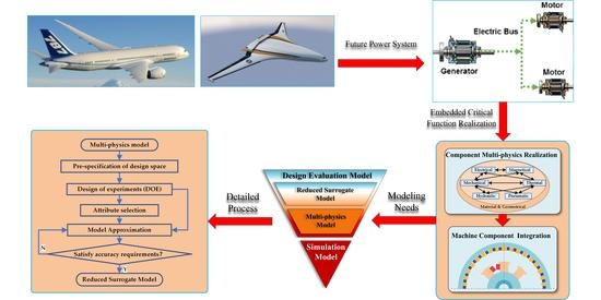
2.1. Modeling Needs Analysis

Traditional machine simulation models calculate variables of power and energy used for the component selections [14]. Both steady-state and dynamic simulations are mandatory due to the complex couplings of multi-physical characteristics. These simulations are usually based on lumped circuit models or field models, and run in environments such as MATLAB/Simulink, Dymola, and ANSOFT. To run this kind of model, it is necessary that all component parameters should be known. Meanwhile, it is highly time-consuming to extract features from models. Therefore, it is suitable for detailed design, analysis, and verification, whereas time-independent symbolic analytical models are preferred for assisting with system integration.

From the perspective of design optimization, design requirements can be translated into design, constraint, and target variables of different levels. Then, the design is conducted hierarchically by algebraic solvers or intelligent algorithms to achieve the best goals with the satisfaction of constraints by well-determined design variables; see Figure 1. As the impacts of variations of variables can be propagated both vertically (from bottom to top, e.g., components, machine, and system) and horizontally (e.g., among components), every design is a combinational optimization problem based on both the underlying design results and the synthesis forms of underlying-level designs, e.g., the selected component technologies and the selected machine structure in the machine design process. Therefore, iterative calculations may occur because of the improper design or integration of the underlying units; in Figure 1, see the red and green-colored directed lines. Therein, the green-colored lines can be avoided by optimization algorithms, whereas the red-colored lines cannot be avoided and may lead to blind designs, due to the invisible and complex cross-links among variables.

Accordingly, the hierarchical designs require a well-structured modeling approach:

• The primary-level model handles the design of the machine for the integration of More-electric systems, linking dimensions and characteristics of selected materials and technologies to multi-physical characteristics of components with full consideration of their energy conversion features [29]. Thus, couplings of variables can be illustrated clearly.
• The secondary-level model allows proper simplification of the primary-level multi-physics model, which focuses on the performance evaluation of the system, and should be consistent with the primary-level model.

In this way, the developed modeling approach covers enough information needed for different levels of design and evaluation, and appears to be the most appropriate means of accelerating the design process, which is the major task and objective of this paper.

2.2. Modular Multi-Physics Model

To demonstrate the propagations of the impacts of variables, both multi-physical characteristics and combinatorial explosions of components are required in the multi-physics model. On the other hand, the modular approach in electrical machines denotes that their parts (the stator, the rotor, or both) are made up of distinctive segments, which can increase flexibility of design. Therefore, the structure of the improved multi-physics model is illustrated in Figure 2.

Every component model comprises three parts, namely, technical parameters, multi-physics coupled constraints, and the design goal, in which the multi-physics coupled constraints represent the core linking the other two parts. Technical parameters comprise the design codes from design experiences, standards, and protocols (i.e., densities and strengths of materials, technology readiness level (TRL), etc.), which are used as pre-specified design requirements. According to the selected configurations in the technical parameters, the multi-physics coupled constraints describe the relationship between design variables and performance according to the principle of energy conversion and transmission; structure parameters describing the geometry and material information can be then obtained. Based on these two parts, the design goal calculates evaluation indexes depending on design requirements.

The component integration model has a similar structure to component models. The difference is in the components coupled constraints describing the cross-links of components. Differently from the traditional machine design method, the machine here is designed based on the direct approach. The detailed process is as follows: according to the required performance (i.e., the rated power, operating points of components, etc.), main radial and axial dimensions are initially calculated by the basic equations of the machine; then, detailed parameters of components (e.g., dimensions of the rotor, stator, yoke, or windings) are determined by optimal technology selections; next, the whole machine is integrated in aspects of structural, electromagnetic, and thermal features; finally, constraints and initial assumptions are checked to verify the design. Calculations in [35] show that the differences between initially assumed parameters and calculated results based on the direct approach are small enough to form the closed loop of design.

In this way, functional and performance characteristics are included and couplings of parameters are demonstrated explicitly in the multi-physics model. With changes in component structures and their integration forms, the trade-off of different machines can be achieved easily. Moreover, design codes are integrated into the model in this paper. Therefore, significant expertise for each component is not required for integrators to implement and shrink the component range to a reduced number of candidate technologies in system-level studies [24].

2.3. MDO-Based Model Simplification

To satisfy the system-level design demands, the MDO method is first used in the simplification of the multi-physics model to generate the simplified model, so that secondary-level models with characteristics of accuracy, simplicity, and consistency can be obtained. This process is illustrated in Figure 3.

By manipulating model inputs according to pre-specified design space, design of experiments (DOE) technology is applied to generate the data sample for the analysis. To describe the whole performance of the multi-physics model effectively, sufficient design points evenly spread in the design space are required. Then the model-based sensitivity analysis method is introduced to explore the design space and find cause-and-effect relationships between the inputs and outputs of the multi-physics model. From the sensitivity analysis, an optimal parameter combination for system-level machine models can be concluded. Based on the data and the optimal selected variable combination, surrogate models, which have been widely used in engineering design due to the low computational cost and high fidelity [36,37], are built for the system-level study. The approximation model can be improved by using better learners and adding additional sample points to achieve better precision.

3. Modular Multi-Physics Model

The variable-speed variable-frequency (VSVF) electrically excited synchronous generator is chosen as the case study to illustrate the improved multi-physics modeling process. The 2D structure of the machine is shown in Figure 4. In this study, the weight and power loss are naturally selected as the objectives. According to the proposed method and [29,35], the improved multi-physics model of machines includes the sub-models as discussed in the following.

3.1. Shaft Model

3.1.1. Multi-Physics Coupled Constraints

The shaft model involves mechanical, structural, and cooling features. The shaft is assumed to be a hollow cylinder, the diameter of which is determined by the electromagnetic power P_em, rotational speed n, and the mechanical properties of the material:

$$D_s=\max \left(\begin{array}{l}{A}_{sh}\sqrt[3]{P_{em}/\left[\left(1-{\alpha }_s^4\right)n\right]}\\ B_{sh}\sqrt[4]{P_{em}/\left[\left(1-{\alpha }_s^4\right)n\right]}\\ \sqrt[3]{F/\left[0.1\left(1-{\alpha }_s^4\right){\left[{\sigma }_{-1}\right]}_b\right]}\end{array}\right)\times {10}^{-3},$$

(1)

where D_s is the outer diameter; A_sh is the coefficient of shear stress; B_sh is the stiffness coefficient of material; [σ₋₁]_b is the admissible bending stress; α_s is the ratio of the inner to outer diameter, and F is the equivalent moment.

P_em can be calculated according to Equations (2) and (3) [38]:

$$P_{em}=\{\begin{array}{l}{K}_{E}P/\cos \phi ,\mathrm{synchronous} \mathrm{generator}\\ K_{E}P/\cos \phi /\eta ,\mathrm{synchronous}/\mathrm{induction} \mathrm{motor}\end{array},$$

(2)

$$K_E=0.931+0.0108\ln P-0.013p,$$

(3)

where P is the rated power; p represents the pole pairs; η is the assumed efficiency; cosφ is the power factor, and K_E is the per-unit value of full-load potential, namely, the ratio of induced electromotive force to the output voltage at full loads.

The gravity center of the rotor is assumed to be at the center of the shaft, and to be at the same position as the circle center of the stator. Thus, F can be calculated according to Equation (4):

$$\{\begin{array}{l}F=\sqrt{F_w^2+0.59F_t^2}\\ F_w=2.45W_r{l}_{ef}\\ F_t=9.55P_c/n\end{array},$$

(4)

where l_ef is the efficient length of machine; F_w is the bending stress caused by the rotor weight W_r, and F_t is the rated torque.

3.1.2. Design Goals

The shaft weight W_sh is shown in Equation (5):

$$\{\begin{array}{l}{V}_{sh}=\pi \left(1-{\alpha }_s^2\right)D_s^2{l}_{ef}/4\\ W_{sh}={\rho }_{sh}{V}_{sh}\end{array},$$

(5)

where V_sh is the shaft volume, and ρ_sh is the material density.

For the VSVF system, the influences of the variable rotational speed should be taken into consideration to ensure security, e.g., the stresses of shaft diameters.

3.2. Yoke Model

3.2.1. Multi-Physics Coupled Constraints

The yoke model involves magnetical, structural, and thermal features. As one of the main dimensions of a hollow cylinder, the yoke’s thickness h_y can be calculated according to the magnetic flux Φ_y and the selected induction B_y. The magnetic potential F_y can be obtained according to the B-H curve of the selected material:

$$\{\begin{array}{l}{h}_y={\Phi }_y/\left(2l_{ef}{k}_c{B}_y\right)\\ F_y=k_c{H}_y\left(2h_y+\pi D_y/p\right)\xi \end{array},$$

(6)

where k_c is the lamination factor [39]; D_y is the average diameter of the yoke; ξ is the length coefficient of the yoke magnetic circuit, and H_y is the yoke magnetic intensity corresponding to B_y.

It is assumed that B_y0 is the yoke induction when the machine is in an idle run, whereas B_yN is the yoke induction when the machine runs at full load. The relationship between B_y0 and B_yN is shown in Equation (7). By Equation (6) and (7), magnetic potentials of the yoke at no load and full load can be calculated. Combined with the magnetic potentials of other components calculated in a similar way, the magnetic circuit can be integrated, and the design requirements of the excitation windings can be obtained.

$$B_{yN}=\left|E_i\right|B_{y0},$$

(7)

where |E_i| is the amplitude of the per-unit value of rated induced electromotive force, and the calculation is introduced in the winding component.

The thermal circuit of the yoke satisfies Equation (8). Note that other components have similar thermal models.

$$\{\begin{array}{l}{T}_y=P_{iron\_y}{R}_y\\ {\displaystyle \int P_y}dt=C_y\Delta T_y\\ P_{y\_o}=P_{iron\_y}-P_{h\_y}\\ C_y=Sp{C}_y{m}_y\end{array},$$

(8)

where T_y is the temperature rise of the yoke; P_{iron_y} is the produced heat by the yoke iron loss; R_y is the thermal resistance of the yoke, which is dependent on the material and proportional to the surface area [20]; P_h__y is the stored thermal power of the yoke; C_y is the yoke thermal capacity, which is the product of the specific heat SpC_y and mass m_y; ΔT_y is the fluctuation of T_y, and P_{y_o} is the thermal power transferring from the yoke to other components.

At the steady heat balance state, as the yoke temperature is fixed, namely ΔT_y = 0, P_{y_o} equals P_{iron_y}, which indicates that the branch of C_y is ignored in the thermal circuit in the design phase.

3.2.2. Design goals

The yoke weight W_y and the iron loss P_y can be calculated according to Equation (9):

$$\{\begin{array}{l}{W}_y=\pi {\rho }_y{l}_{ef}{D}_y{h}_y/2\\ p_y=p_{10/50\_y}{B}_y^2{\left(f/50\right)}^{1.3}\\ P_y=k_{a\_y}{p}_y{W}_y\end{array},$$

(9)

where ρ_y is the density of the yoke material; p_y is the yoke iron loss per kilogram; f is the operating frequency; p_{10/50_y} is the yoke iron loss when B = 1 T and f = 50 Hz, and k_{a_y} is the empirical coefficient, usually determined by Equation (10) [35]

$$k_{a\_y}=\{\begin{array}{l}3.6, \mathrm{DC} \mathrm{machine} \mathrm{or} P<100 \mathrm{kVA} \mathrm{AC} \mathrm{machine}\\ 1.3, P>100 \mathrm{kVA} \mathrm{AC} \mathrm{machine}\end{array}.$$

(10)

3.3. Slot Model

3.3.1. Multi-Physics Coupled Constraints

The slot model involves structural, magnetical, and thermal features. The shape of slots is selected based on the rated power P and armature winding voltage E by experience; see Equation (11) [38]:

$$\{\begin{array}{l}E>1000 \mathrm{V}\Rightarrow \mathrm{open} \mathrm{slot}\\ E<1000 \mathrm{V} \& P>30 \mathrm{kW}\Rightarrow \text{semi-open} \mathrm{slot}\\ E<500 \mathrm{V} \& P\le 30 \mathrm{kW}\Rightarrow \text{semi-closed} \mathrm{slot}\end{array},$$

(11)

where it is assumed that the slot induction B_s equals the induction at a one-third height of the slot from the dedendum; see Figure 4. According to Equation (12), the magnetic potential of slots F_s can be calculated:

$$\{\begin{array}{l}{b}_s=\pi D_a{B}_{\delta }/\left(2Z{k}_c{B}_s\right)\\ F_s=2k_c{H}_s{h}_s\end{array},$$

(12)

where Z is the slot number; b_s and H_s are, respectively, the tooth width and magnetic intensity corresponding to B_s, and h_s is the slot height.

The slot inductions at no load and full load B_s0 and B_sN satisfy

$$B_{sN}=\left|E_i\right|B_{s0}.$$

(13)

3.3.2. Design Goals

Sections of every slot are assumed to be trapezoidal; thus, the slot weight W_s and the iron loss P_s can be calculated according to Equation (14):

$$\{\begin{array}{l}{W}_s=Z{\rho }_y{l}_{ef}\left(b_Z+b_d\right)h_s/2\\ Z=2mp{N}_Z\\ b_d/\left(D_a/2+h_s\right)=2b_Z/D_a=b_s/\left(D_a/2+2h_s/3\right)\\ p_s=p_{10/50\_s}{B}_s^2{\left(f/50\right)}^{1.3}\\ P_s=k_{a\_s}{p}_s{W}_s\end{array},$$

(14)

where ρ_s is density of the yoke material; b_z and b_d are the widths of the addendum and dedendum respectively; N_Z is the slot number per pole per phase; m is the phase number; D_a is the bore diameter; p_s is the slot iron loss per kilogram; p_{10/50_s} is the yoke iron loss when B = 1 T and f = 50 Hz, and k_{a_s} is the empirical coefficient, usually determined by Equation (15) [35]:

$$k_{a\_s}=\{\begin{array}{l}4, \mathrm{DC} \mathrm{machine} \\ 1.8, \mathrm{induction} \mathrm{machine} \\ 2, P<100 \mathrm{kVA} \mathrm{synchronous} \mathrm{machine}\\ 1.7, P>100 \mathrm{kVA} \mathrm{synchronous} \mathrm{machine}\end{array},$$

(15)

3.4. Air-Gap Model

Multi-Physics Coupled Constraints

The air-gap model involves structural, magnetical, and thermal features. The air-gap thickness δ, coefficient k_δ, and magnetic potential F_δ are illustrated in Equation (16) [38]:

$$\{\begin{array}{l}\delta =0.36A\tau /\left[\left(x_d^{\ast }-1\right){\Phi }_{\delta }\right]\times {10}^{-6}\\ k_{\delta }=\left(\pi D_a/Z+10\delta \right)/\left(b_Z++10\delta \right)\\ F_{\delta }=k_{\delta }{B}_{\delta }\delta /{\mu }_0\end{array},$$

(16)

where A is the electric loading; τ is the pole pitch; $x_d^{\ast }$ is the relative direct-axis inductance, ranging from 1.1 to 1.4; Φ_δ is the air-gap magnetic flux; μ₀ is the permeability of vacuum, and B_δ is the air-gap induction:

$$B_{pN}=\left|E_i\right|B_{p0},$$

(17)

where B_δ0 and B_δN are the air-gap inductions at no load and full load.

As the oil spray cooling method is chosen for this machine, the equivalent thermal circuit of cooling oil is included in the thermal model of the air gap. To simplify the calculation, it is assumed that the oil is coated evenly on the surfaces of the stator and rotor.

3.5. Pole Model

3.5.1. Multi-Physics Coupled Constraints

The pole model involves magnetical, thermal, and structural features. The shape of the poles is determined by the machine type.

In this article, as the study case is a salient pole synchronous machine, the pole shape is illustrated in Figure 4. It is assumed that the pole shoes are of the same circle center as the rotor yoke, and its width is assumed to be equal to τ. Then, the pole-core width b_p can be calculated by exciting flux Φ_p and selected pole induction B_p. The magnetic potential of pole F_p can be calculated by the corresponding magnetic intensity H_p and pole height h_p. Therein, B_p has the same meaning as the afore-mentioned B_y; see Equation (19):

$$\{\begin{array}{l}{b}_p={\Phi }_p/\left(B_p{l}_{ef}{k}_c\right)\\ F_p=k_c{H}_p{h}_p\end{array},$$

(18)

$$B_{pN}=\left|E_i\right|B_{p0},$$

(19)

where B_p0 and B_pN are the pole inductions at no load and full load, respectively.

For a PMSG, the volume of the permanent magnet V_m can be estimated by the Larionoff method; see Equation (20) [38]. For the non-salient pole synchronous generator, the volume is calculated via the unsaturated vectogram, which is omitted here.

$$V_m=K_{bh}{P|}_{\cos \phi =0}{K}_{\sigma 0}{K}_{adF}{K}_K^2/\left(f{B}_r{H}_C\right)/\left(K_K-1\right),$$

(20)

where K_bh is a coefficient related to the material and selected operating point of the poles, and pole-arc coefficient, etc.; P|_{cosφ = 0} is the rated power when the power factor is zero; K_σ0 is the leakage flux coefficient at no load, and is dependent on the rotor structure, material, and pole pairs; K_adF is the equivalent coefficient of armature potential, which is dependent on the pole material; B_r and H_C are the remanent induction and coercive force of the pole material, respectively; K_K is the short-circuit current ratio.

Detailed dimensions can be calculated according to the pole structure (shape and magnetization direction); the process is omitted here but can be found in [35].

The selection of the operating point of poles is based on the material, including its magnetic and thermal characteristics. It is assumed that the demagnetization curve of the selected material is linear; thus, the operating point of poles (B_m,H_m) can be calculated by Equations (21) and (22):

$$\{\begin{array}{l}{B}_{rT}=B_{r0}\left[1-\left|{\alpha }_B\right|\left(T-T_0\right)\right]\\ H_{CT}=H_{C0}\left[1-\left|{\alpha }_B\right|\left(T-T_0\right)\right]\\ {\alpha }_B=\left(B_{rh}-B_{rl}\right)/B_{rl}/\left(T_h-T_l\right)\end{array},$$

(21)

where B_rT and H_CT are the remanent induction and coercive forces at temperature T, respectively; B_r0 and H_C0 are the remanent induction and coercive forces at standard temperature T₀, respectively; α_B is the temperature coefficient of remanence; T is the actual operating temperature; T_h and T_l are the upper and lower limits of the allowed temperature, respectively, and B_rh and B_rl are the inductions at T_h and T_l, respectively. The influence of temperature on the irreversible magnetic degradation is ignored here.

$$\{\begin{array}{l}{B}_m=K_{\sigma }{B}_{rT}/2\\ H_m=\left(1-K_{\sigma }/2\right)H_{CT}\end{array},$$

(22)

where K_σ is the leakage flux coefficient.

3.5.2. Design Goals

The pole weight W_p and the iron loss P_p can be calculated according to Equation (23):

$$\{\begin{array}{l}{W}_p={\rho }_p{V}_m\\ p_p=p_{10/50\_p}{B}_p^2{\left(f/50\right)}^{1.3}\\ P_p=p_p{W}_p\end{array},$$

(23)

where ρ_p is the density of the pole material; p_p is the pole iron loss per kilogram, and p_{10/50_p} is the pole iron loss when B = 1 T and f = 50 Hz.

3.6. Winding Model

3.6.1. Multi-Physics Coupled Constraints

The winding model involves electromagnetic and thermal features. The configurations of the armature winding are determined by optimally selecting the magnet wire based on the carrying capacity, which is calculated by the rated power P, the armature winding voltage E, the pitch ratio β, and the current density J_a, whereas those of the excitation winding is determined by the excitation magnetic potential F_f and current density J_f.

In detail, the number of winding turns in series N is determined by E, and the number of paralleled conductors a can be calculated according to the standard MIL-W-5088L and the wire gauge standard [40]; see Equation (24):

$$\{\begin{array}{l}E=4.44fN{k}_W\Phi \\ k_W=\sin \left(\pi \beta /2\right)\sin \left(q\alpha /2\right)\\ q=Z/\left(2pm\right),\alpha =2\pi p/Z\\ I=\pi aJ{d}^2{k}_{sh}{k}_g{k}_T\end{array},$$

(24)

where f is the frequency of the output voltage; k_W is the winding coefficient; Φ is the main magnetic flux; β is the ratio of the winding pitch to the polar pitch τ; q is the number of slots per pole per phase; α is the electrical angle; m is the phase number; J is the current density of the selected wire gauge; d is the diameter of the selected wire gauge; k_sh is the bundling coefficient of conductors; k_g is the altitude correction coefficient of conductors, and k_T is the temperature coefficient of conductors.

According to the requirements of the wire insulation [41], the diameter of the selected electromagnetic wire d_ew satisfies Equation (25):

$$\{\begin{array}{l}t{h}_{ins}=E/{\epsilon }_{ew}\\ d_{ew}=d+2t{h}_{ins}\\ d_{ew}\le d_{\max }\end{array},$$

(25)

where d_max is set as the maximum wire diameter allowed for an inlay technology reason, and ε_ew is the dielectric strength of the insulation.

According to the first-order model of the machine [42], the resistance and inductance can be calculated; see Equations (26) and (27):

$$\{\begin{array}{l}{R}_a=k_{r}N{\rho }_c{l}_c/s_c/a\\ {\rho }_c={\rho }_0\left(1+{\alpha }_c\Delta T\right)\end{array},$$

(26)

where R_a is the resistance of the armature winding; k_r is the coefficient considering the skin effect, which is dependent on the shape, configuration, and frequency of conductor; ρ_c is the electrical resistivity of the conductor, which is dependent on the material (electrical resistivity at 20 °C ρ₀ and temperature coefficient α_c) and temperature rise ΔT, and l_c and s_c are the average conductor length and area per turn, respectively.

$$\{\begin{array}{l}{X}_m=4f{\mu }_0{N}^2{l}_{ef}{\lambda }_m/\left(pq\right)\\ X_M=-4f{\mu }_0{N}^2{l}_{ef}{\lambda }_M/\left(pq\right)\\ X_{\sigma }=4f{\mu }_0{N}^2{l}_{ef}\left({\lambda }_s+{\lambda }_{\delta }+{\lambda }_t+{\lambda }_E\right)/\left(pq\right)\\ X_a=X_m-X_M+X_{\sigma }\end{array},$$

(27)

where X_m, X_M, X_σ, and X_a are the main, mutual, leakage, and total inductances of the armature winding, respectively; the specific permeance coefficients λ_m, λ_M, λ_s, λ_δ, λ_t, and λ_E are dependent on the slot shape and configurations of windings; detailed expressions are omitted here due to the existence of multiple kinds of combined constructs [35].

To integrate the magnetic circuit, the per-unit value of the rated induced electromotive force E_i, which is a gain coefficient to obtain the rated operating points of every component, is calculated according to the impedance of armature windings [29]; see Equation (28):

$$\{\begin{array}{l}{R}_a^{\ast }=R_{a}P/E^2,X_{\sigma }^{\ast }=X_{\sigma }P/E^2\\ E_i=W+\mathrm{j}Q=\sqrt{W^2+Q^2}{e}^{j\epsilon }\\ W=1+R_a^{\ast }\cos \phi +X_{\sigma }^{\ast }\sin \phi \\ Q=X_{\sigma }^{\ast }\cos \phi -R_a^{\ast }\sin \phi \\ \epsilon =\arctan \left(Q/W\right)\end{array},$$

(28)

where $R_a^{\ast }$ and $X_{\sigma }^{\ast }$ are the per-unit value of R_a and X_σ, respectively; W and Q are the real and imaginary parts of E_i, respectively, and ε is the phase angle of E_i.

In addition, the winding thermal model includes the thermal circuit of both wire and insulation.

3.6.2. Design Goals

According to the determined strands of wires, the weight W_aw and power loss P_aw can be calculated; see Equation (29):

$$\{\begin{array}{l}{W}_{aw}=mNa{W}_{aw\_s}\\ W_{aw\_s}=\pi \left(l_{ef}+\tau \right)\left[{\rho }_{ew}{d}^2+{\rho }_{ins}\left(d_{ew}^2-d^2\right)\right]/2\\ P_{ew}=m{I}^2{R}_a\end{array},$$

(29)

where W_{aw_s} is the weight of single-strand wire, and ρ_ew and ρ_ins are the densities of conductor and insulation materials, respectively.

3.7. Integration Model

3.7.1. Components Coupled Constraints

The whole machine model is integrated into aspects of structural, magnetical, and thermal features.

The structural integration is mainly focused on the radial dimensions of components, including the main geometrical parameter shown in Equation (30), constraints of lengths shown in Equation (31), and the space-filling of windings shown in Equation (32):

$$\{\begin{array}{l}CA=D_a^2{l}_{ef}/\left(P_{em}/n\right)=6.1/\left({\alpha }^{\prime }{k}_{W}A{B}_{\delta }\right)\\ \lambda =l_{ef}/\tau \\ D_{sy}=D_a+K_p\tau \end{array},$$

(30)

where CA is the machine constant; D_a is the diameter of the armature; λ is the dimension ratio; the pole-arc coefficient α’ is assumed to be 2/π, which results in a sinusoidal magnetic field; D_sy is the stator outer diameter, and K_p is an empirical coefficient related to p.

As component dimensions are calculated by their respective inductions, when components are integrated into the structure, implicit constraints exist among inductions of components to make sure that they can be put in a limited space. Therefore, component inductions should be properly selected to satisfy Equations (31) and (32):

$$\{\begin{array}{l}{h}_s=\left(D_{sy}-D_a\right)/2-h_{sy}>0\\ h_p=\left(D_a-D_s\right)/2-h_{ry}>0\end{array},$$

(31)

$$\{\begin{array}{l}{b}_p/2+a_w+b_w\tan \mathsf{\theta }=r_r\sin \mathsf{\theta }\\ 0<b_w\le r_r\cos \mathsf{\theta }-\left(D_s/2+h_{ry}\right)\\ r_r=D_s/2+h_{ry}+h_p\\ \mathsf{\theta }=\mathsf{\pi }/2/p\\ 40\%\le K\le 80\%\end{array},$$

(32)

where h_sy and h_ry are the thicknesses of the stator and rotor yoke, respectively; a_w and b_w are the tangential and radial lengths of excitation windings, respectively; r_r is the radius of the rotor; θ is one-quarter of the mechanical angle of machine, and K is the slot fill factor.

The magnetical integration calculates the magnetic circuit, and the excitation requirement is obtained by adding the no-load and full-load magnetic potentials of components; see Equation (33):

$$\{\begin{array}{l}{F}_a=1.1\left(F_{\delta }+F_s+F_{ry}+F_p+F_{sy}\right)\\ F_f=1.05F_a\sqrt{1+{\left(F_{ad}/F_a\right)}^2+2F_{ad}/F_a\sin \left(\phi +\epsilon \right)}\end{array},$$

(33)

where F_ry and F_sy are the magnetic potentials of rotor yoke and stator yoke, respectively; F_a is the magnetic motive force of armature winding, and F_ad is the direct-axis magnetic motive force of armature winding; detailed expressions are omitted here as this is a complex equation.

The thermal integration illustrates the thermal behavior of every component (slot, yoke, etc.) with respect to their resistances, capacities, and ambient conditions, by a thermal circuit, which is coupled with electromagnetic characteristics through losses; see Figure 5. Requirements of the cooling system, e.g., the flow rate of the cooling oil [43], can be deduced from Equation (6) by calculating the thermal resistance and capacity of cooling oil R_co and C_co, which offers a resting interface to the fuel pump system. In addition, the thermal load AJ_a is also given as a constraint here.

3.7.2. Design Goals

The total weight W_G and power loss P_G are calculated by Equation (34):

$$\{\begin{array}{l}{W}_G=W_{sh}+W_{ry}+W_{ew}+W_p+W_s+W_{aw}+W_{sy}\\ P_G=P_f+P_{aw}+P_{ew}+P_{ry}+P_p+P_s+P_{sy}+P_{\Delta }\end{array},$$

(34)

where W_ry, W_ew, W_aw, and W_sy are the weights of the rotor yoke, excitation windings, armature windings, and stator yoke, respectively; P_ew and P_aw are the copper loss of excitation and armature windings, respectively; P_ry and P_sy are the iron loss of the rotor and stator yoke, respectively; P_Δ is the stray loss, and is assumed to be one percent of the rated power, and P_f is the total friction loss; see Equation (35) [44].

Therein, the rotor is assumed to be a cylinder when the windage friction loss is calculated:

$$\{\begin{array}{l}{P}_f=P_{sb}+P_{air}\\ P_{sb}=1.05Fn\times {10}^{-4}\\ P_{air}={\rho }_{air}{\left(D_a-2\delta \right)}^4{\omega }^3\left[K_{f1}\pi l_{ef}+K_{f2}\left(D_a-2\delta \right)/8\right]\\ {\rho }_{air}=1.293p_{ress}/\left(1+0.00367T\right)/760\end{array},$$

(35)

where P_sb and P_air are the friction losses of bearing and windage, respectively; ρ_air is the air density at temperature T (°C) and pressure p_ress (mmHg); ω is the angular velocity of the rotor, and K_f1 and K_f2 are the friction coefficients of the cylinder and disk, and are dependent on the Couette Reynolds Number Re.

It is assumed that K_f1 and K_f2 are equal to K_f, and K_f can be calculated by Equation (36) [45]:

$$K_f=\{\begin{array}{l}0.515C_r{\left[\delta /\left(D_a-2\delta \right)\right]}^{0.3}R{e}^{-0.5},500<Re<{10}^4\\ 0.0325C_r{\left[\delta /\left(D_a-2\delta \right)\right]}^{0.3}R{e}^{-0.2},Re>{10}^4\end{array},$$

(36)

where C_r is the relative roughness coefficient of the rotor, and is assumed to be 1, and Re is obtained according to Equation (37):

$$Re={\left(D_a-2\delta \right)}^2\omega /\nu ,$$

(37)

where ν is the kinematic viscosity of the airflow.

3.8. Summary

3.8.1. Problem Definition

The machine design problem can be sorted into the forms illustrated in Equation (38) by the equations above.

$$\begin{array}{l}Min \left[W_G,P_G\right]\\ s.t.\\ \mathrm{Explicit}: \text{multi-physics} \mathrm{couplings} \mathrm{of} \mathrm{components}\\ \mathrm{Implicit}: \{\begin{array}{l}\mathrm{structural} \mathrm{couplings} \mathrm{among} \mathrm{components}\\ \mathrm{initial} \mathrm{assumptions} \mathrm{verification} \end{array}\end{array}$$

(38)

where the weight, power loss, physical dimensions, and cost of the generator are usually the major design goals of a machine in aircraft applications. In this study, the weight and power loss are naturally selected as the objectives, and the physical dimension of the machine is given in the process of modeling. As the cost can be calculated by multiplying the material price by the weight [44], it is omitted here. Detailed calculations are included in the design goal of every modeling module.

As illustrated in the constraints of every modeling module, the machine has electromagnetic, structural, and thermal features, and the constraints of the problem include multi-physics couplings inside and among components. They can be divided into two kinds, namely, explicit and implicit. The explicit constraints are those expressions in which the outputs can be represented by inputs without iterative calculations, e.g., Equation (1), whereas implicit constraints are those expressions that cannot, e.g., Equation (31). Explicit constraints can be substituted into the goal functions directly, whereas implicit ones cannot. Therefore, considering that the search algorithm has the ability to achieve optimal solutions, if the implicit constraints are not satisfied, the model outputs high penalty factors to break the re-design loop to simplify the calculation.

3.8.2. Model Improvements

Compared with other models, the developed multi-physics model is improved as follows:

• The model is restructured and divided into several replaceable modules to illustrate the couplings of components. Thus, other machine types can be evaluated easily just by changes in shape, material, and radial positions of component modules, which also follows the concurrent design concept.
• Design codes, e.g., the wire gauge, shape selection experiences, and empirical formulas are embedded to realize easier designs for system integrators.
• Inputs are well selected according to the insulation requirements, which offer comprehensive links with practical design requirements, whereas penalty coefficients are used to break the closed loops of the design, which simplifies the calculation.

However, the dimensionality of the built model is greater than that of the model in [29]. This is because some design variables are not independent, e.g., component inductions. For the purpose of power system integration, this high-dimensional design space clearly leads to difficulties in the trade-off. Therefore, simplification is needed to improve the design efficiency.

4. Model Simplification

To further reduce the dimensionality of the built multi-physics model, this section explores its design space by sensitivity analysis methods and then establishes the simplified models used for system integration based on the model approximation technologies. To illustrate this process clearly, materials and empirical coefficients are pre-specified (the 45 carbon steel made shaft, the D41 cold-rolled silicon steel sheet, the fluoropolymer coating insulation, the ratio of the inner and outer diameter, and relative direct-axis inductance, etc.). Variation ranges of other undetermined design variables are listed in

Table 1. Variation ranges of the built generator model.

Design Variables	Lower Levels	Upper Levels
P (kW)	30	300
p	1	6
β	2/3	7/8
cosφ	0.8	0.9
n (r/min)	1000	30,000
λ	0.6	4
ΔT (°C)	0	105
A (A/m)	2.3 × 104	6 × 104
Bp (T)	1.3	1.7
Bry (T)	1.15	1.7
Bst (T)	1.5	2
Bsy (T)	1.35	1.75
Bδ (T)	0.6	1
Ja (A/mm2)	7	11
Jf (A/mm2)	4.5	9
E (V)	115	5000
AJa (A/m∙A/mm2)	2 × 105	5 × 105

, according to the requirements of Class F insulation.

To implement the simplification, a data set, which can efficiently describe the whole performance of the multi-physics model, is required. To obtain the data set, the optimal Latin hypercube design (LHD) algorithm [46,47,48] is applied and the discrepancy of point sets is selected as the optimized criterion objective to generate a design matrix evenly spread in the design space presented in Table 1. To facilitate an accurate analysis, a matrix of 10,000 points is used here. The process is demonstrated in Figure 6. With the increase of design points, the discrepancy of point sets declines evidently first and then remains steady after 800 iterations. Then, by substituting the design points into Equation (38), corresponding outputs of the multi-physics model are obtained. As constraints are not always satisfied, 990 unsuitable points are eliminated before the analysis. As every iteration generates nine points on average, the remaining 9010 design points can be regarded as the results at the 1001st iteration in Figure 6, which verifies the distribution performance of this filtered data set.

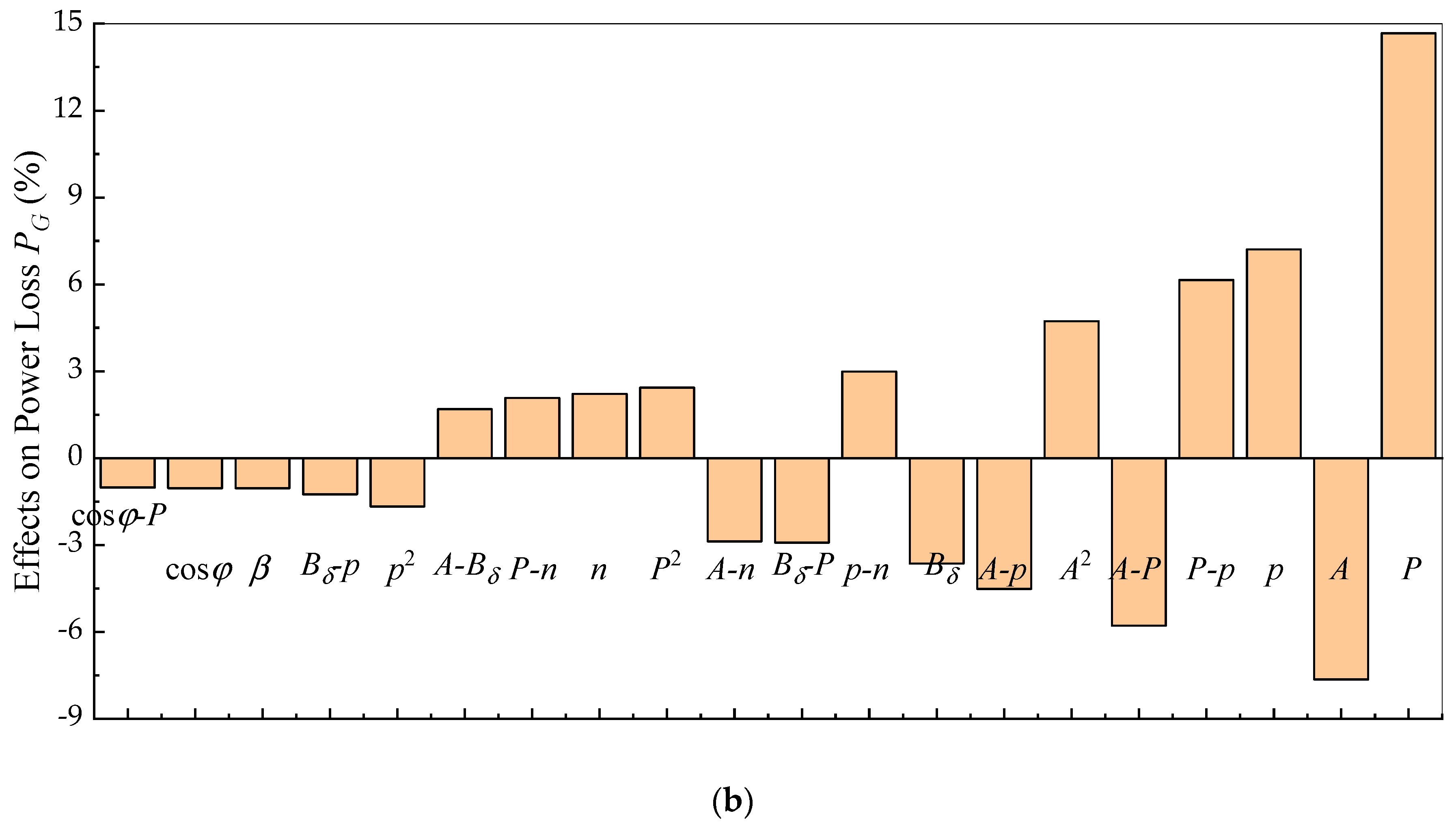
4.1. Sensitivity Analysis

To obtain the optimal parameter combination, this paper analyzes trends between inputs and outputs to identify key factors of the multi-physics model by the multiple quadratic regression method.

Equation (39) illustrates the principle of this method with a binary quadratic function. The differential of y can be divided into main and interaction effects of x₁ and x₂. For example, coefficients c₁ and 2c₃ can reflect the main effects of x₁ on y; c₂ and 2c₄ can reflect the main effects of x₂ on y, and c₅ can reflect the interaction effect of x₁ and x₂ on y. Therefore, based on the multiple quadratic regression model, the influences of design variables on the weight and power loss can be evaluated:

$$\{\begin{array}{l}y=c_0+c_1{x}_1+c_2{x}_2+c_3{x}_1^2+c_4{x}_2^2+c_5{x}_1{x}_2\\ dy=c_{1}d{x}_1+c_{2}d{x}_2+2c_{3}d{x}_1+2c_{4}d{x}_2+c_{5}d\left(x_1{x}_2\right)\end{array}$$

(39)

The determination coefficient (R²) is used to evaluate the imitative effect of the multiple quadratic regression model. The R² of the weight and power loss models are 0.9705 and 0.97848, respectively, which indicates the accuracy of the analysis.

Figure 7 illustrates the main factor plots of weight and power loss. The main factors of the weight W_G are the rotational speed n, rated power P, pole pairs p, and electric loading A, whereas those of the power loss P_G are the rated power P, electric loading A, pole pairs p, rotational speed n, and air-gap induction B_δ. Both weight and power loss rise linearly with the increase of the rated power. Moreover, with the rise of pole pairs, the weight declines whereas the power loss increases. In addition, it is notable that the voltage has few effects on weight and power loss.

Due to different dimensions and ranges of variables, dimensionless processing is executed to achieve fair identification of couplings; the top 20 contributors of design variables and couplings are shown in Figure 8. The weight attributes 83.05% of itself to the couplings of the rated power P, pole pairs p, rotational speed n, electric loading A, air-gap flux density B_δ, and pitch ratio β, whereas the power loss attributes 79.35% of itself to the couplings of the rated power P, pole pairs p, rotational speed n, electric loading A, air-gap flux density B_δ, pitch ratio β, and power factor cosφ.

According to the analysis above, some design variables can be ignored, and model inputs before and after the dimensionality reduction are demonstrated in

Table 2. Candidate variables for simplified models.

Models		Alternative Inputs
Before	WG	P, p, A, n, Bδ, β, cosφ, Bp, Bry, Bst, Bsy, Ja, Jf, λ, and E
	PG
After	WG	P, p, A, n, Bδ, and β
	PG	P, p, A, Bδ, n, β, and cosφ

. The dimensionalities of the weight and power loss models can be reduced from 15 to 6 and 7, respectively. As the input variables of the simplified model are the subset of those of the multi-physics model, they have a consistent interface. For a more comprehensive simplification, the pre-specified parameters can be added into the analysis.

4.2. Model Approximation

According to the reduced input variables in Table 2, the methods of radial basis function (RBF) and quartic response surface model (RSM) are used for the approximations of the data sample generated from DOE. Ten-fold cross-validations are executed by randomly partitioning the sample into nine training subsets to train the model and one test subset to evaluate it.

Comparisons between the built models and the test subsets are illustrated in

Table 3. Cross-validation error results of surrogate models.

Models	Evaluation Indexes	RBF	RSM
WG	R2	0.959	0.783
	Average Error 1/%	2.75	13.12
	Max Error 1/%	18.29	29.29
	RMSE 2	0.06	0.16
PG	R2	0.939	0.98
	Average Error/%	6.701	2.44
	Max Error/%	14.79	11.32
	RMSE	0.076	0.0394

¹ Max and average error are both calculated by absolute values of relative errors. ². Root mean square errors (RMSE) are calculated after normalizations, varying from 0 to 1.

. The RSM-based weight model has a relatively low accuracy and high degree of uncertainty, whereas other models achieve satisfactory results. As only a small amount of data is required by the approximation of the reduced-order quartic RSM-based model, the sample containing 9010 points cannot be covered. Accordingly, although ten-fold cross-validation helps keep models accurate by calculating multiple surrogate models of different subsets, the performance of reduced-order RSM-based models is worthless for large sample data. In other words, RBF-based surrogate models are preferred.

5. Analysis

5.1. Verification

To verify the modeling method, the auxiliary power unit generator (APUG) in a Boeing 787 with known parameters (apparent power P_s = 225 kVA, electric loading A = 60,000 A/m, pole pairs p = 2, rotational speed n varies in the range of 10,800–24,000 r/min, nominal speed n_N = 12,000 r/min, air-gap induction B_δ+ = 0.8 T, pitch ratio β = 0.75, rated voltage E = 230 V, weight W_G = 52 kg, power loss P_G = 20 kW when n = 24,000 r/min and power factor cosφ = 0.85) [49] is used as the case study.

According to the method, the multi-level models are established. As some inputs of the multi-physics model, e.g., operating points B_p, B_ry, B_st, B_sy, J_a, and J_f, and the dimension ratio λ, are not given, the uncertainties clearly result in a Pareto set. Therefore, according to ranges of the uncertain variables in Table 1, NSGA-II (non-dominated sorting genetic algorithm II) with 100 populations and 1000 generations is used, and the Pareto plot comprised of 3171 points obtained is illustrated in Figure 8. The design results of simplified models and the actual solution are also shown in Figure 9. Therein, two optimal solutions (M1 and M2) on the Pareto plot of the multi-physics model are given as examples for the convenience of the analysis.

5.1.1. Multi-Physics Model Analysis

The actual solution is nearly located on the Pareto plot of the multi-physics model with the minimum errors (0.006% of the weight and 2.7% of the power loss, compared with solution M2), which verifies the multi-physics model. The uncertainties lead the calculated weight to a variation ranging from −3.82% to 4.15% and the power loss to a variation ranging from −2.56% to 16.27% of the actual solution, which suggests that the weight of optimal solutions varies less than the power loss. Therefore, although the decision-making model is not studied here, more importance will be attached to the power loss by designers.

5.1.2. Dimensionality Reduction Analysis

To verify the dimensionality reduction of simplified models, data distributions of design variables of the optimal solutions are analyzed. As the power of the excitation system is relatively low and leads to few fluctuations of the results, their design variables are ignored here.

It is noteworthy that the Pareto set can be divided into two parts with the demarcation point M1 by the dimension ratio λ; see Figure 9. Figure 10 demonstrates the data distribution of the dimension ratio λ in the two parts. It can be concluded that a value of the dimension ratio λ exists in the range from 1.263 to 1.267 as the extreme point of the weight model, whereas it exists in the range from 1.591 to 1.593 as the extreme point of the power loss model. The selection of the dimension ratio is determined by the designer, depending on which index is more important. According to the power loss-preferred design, solutions of the 1728 blue-colored circle points in Figure 9 are probably better choices.

Figure 11 illustrates the data distributions of component operating points in preferred optimal schemes. To achieve the best design results, values of pole and rotor yoke inductions (B_p and B_ry) should be at the upper level, whereas those of stator slot and yoke inductions (B_st and B_sy) should be at the lower level, as shown in Figure 11a–d. It indicates that inductions B_p, B_ry, B_st, and B_sy have few influences on the upper-level designs if the machine is well integrated. Therefore, they are local design variables, which can be ignored in the system-level design. In contrast, values of the current densities are spread relatively evenly in the full ranges given in Table 1, compared with other variables; see Figure 11e–f. The maximum changes of weight and power loss resulting from variations of the armature winding current density J_a and the excitation winding current density J_f are 6.88% and 1.91%, respectively, which suggests that current densities can also be ignored. In addition, it is notable that the models are convex functions of the current densities, as few data exist for the current densities of the armature and excitation windings in the ranges of 7.2–7.6 and 5–6.5 A/mm², respectively.

In conclusion, among the undetermined design variables, λ has a relatively large influence on the weight and power loss, but can be ignored with a high-weighted coefficient of power loss considered in the design and evaluation, whereas component operating points (B_p, B_ry, B_st, B_sy, J_a, and J_f) can also be reduced due to the optimal design results with few variations. Therefore, the dimensionality reduction is proved conclusive.

5.1.3. Simplified Model Analysis

Compared with the actual solution, the errors of the simplified weight and power loss models are acceptably low, at 1.06% and −2.03%, respectively. As the surrogate model is a ‘black-box’ model, the established models are of low complexity. Compared with the weight and power loss of simplified models, the relative variation ranges of the optimal solutions obtained from the multi-physics model on the right of M1 are −3.574–3.067% and −0.526–5.299% respectively, which indicates that the models output almost the same results. In summary, they are proved to be accurate, simple, and consistent.

In conclusion, the simplification is proved to be reliable, and the multi-physics model and simplified models are of high accuracy and consistency.

5.2. Comparisons

In order to demonstrate the superior performance of the proposed modeling method in an application of aircraft power systems, the proposed modeling method is compared with the baseline model of the permanent magnet synchronous motor (PMSG) in [29] and the SL-based model of PMSM in [30].

As the design of the whole aircraft power system is a multi-disciplinary problem resulting from strongly coupled parameters, to achieve the maximum benefit, global optimization solutions are the targets of designers, which indicates that all design variables should be considered at the system level. However, the large amount of on-board equipment leads system-level variables to a high-dimensional design space. Therefore, in addition to the precision, the dimensionality of design space is selected as the compared index to evaluate the performance of the model in system-level applications. As the calculation speed cannot be assessed in the same condition, the complexities of models are compared simply in theory.

5.2.1. Comparison with the Baseline Model

To model the PMSG, we replace the electrical excitation modules (silicon steel pole modules and excitation winding modules) by NdFeB magnet poles, and obtain the simplified PMSG model. Design variables are deduced and obtained combining parameters in [29] and equations in this paper, e.g., rated power P = 7.753 kW, pole pairs p = 3, rotational speed n = 735.2 r/min, electric loading A = 3.69 × 10⁴ A/m, air-gap flux density B_δ = 0.856T, and pitch ratio β = 2/3.

According to the improvements of the model mentioned in Section 3.8, the influences of the structure change on the accuracy can be ignored due to the modular modeling structure, whereas those of the integration of design codes and extended input variables remain to be considered, e.g., impacts of different empirical formulas for the calculation of air-gap lengths. As detailed information is not given, only the total model behaviors are compared; see

Table 4. Model results and error comparisons.

Parameters	Prototype in [29]	FEM in [29]	Multi-Physics Model in [29]	Proposed Simplified Model	Errors of FEM in [29]/%	Errors of Multi-Physics Model in [29]/%	Errors of Proposed Models/%
Ra (Ω)	0.14	0.14	0.13	0.1348	0	7.14	3.71
La (mH)	1.42	1.4	1.37	1.34	1.41	3.52	5.63
δ (mm)	1.8	1.17	1.17	1.853	35	35	2.94
lef (mm)	48.5	48.6	48.6	47.4	0.21	0.21	2.27
Da (mm)	141	-	-	137.6	-	-	2.41
Dsy (mm)	211.3	-	-	193.6	-	-	8.38
WG (kg)	9.8	-	-	9.04	-	-	7.76

. It can be noted that, compared with the prototype, there is a remarkable agreement between the results of the proposed simplified model and the corresponding models in [29].

The input number of the weight model in [29] is eight, whereas that of the simplified weight model in this paper is six, which indicates that a lower dimensionality of design space is needed to be considered in the system-level studies using the proposed method, leading to easier designs. Therefore, with the help of the proposed model, lower computational cost and faster development with considerable accuracy can be achieved.

Moreover, the ‘black-box’ characteristic of the proposed model indicates that its calculation speed is clearly superior to that of the baseline model.

5.2.2. Comparison with the SL-Based Model

To model the PMSM, we change the radial positions of the pole module and slot/armature winding modules inside the PMSG model. As products in [50,51] are of the same series, one reference is selected to identify the variables of the built model, e.g., the electric loading A = 5.62 × 10 ⁴ A/m, air-gap flux density B_δ = 0.85 T, and pitch ratio β = 2/3; these values can be used for the whole series.

The relationship between the rated torque and weight is demonstrated in Figure 12. It can be concluded that, although the actual weight includes external accessories besides the active mass, e.g., the resolver and cable, both models achieve results with relatively high accuracy.

The SL-based method requires three inputs for the weight calculation, i.e., rated torque and weight of the reference machine, and rated torque of the machine to be calculated, which is less than the input number of our model. The power loss estimation requires 10 inputs, i.e., values of power and efficiency of the reference in two different conditions of loads (torque and speed) to calculate the coefficients of the Joule loss and iron loss, and torque and speed of the machine to be calculated. The total required input number of the SL-based method is greater than that of the proposed model.

The SL-based model is comprised of several simple polynomials and some data, whereas the proposed model is a relatively complex data network. Therefore, although they have a similar calculation speed, the occupied memory of the proposed model is higher than that of the SL-based model in the optimization process, which can be ignored compared with the generated solutions.

Moreover, the SL-based model cannot reflect the couplings of multi-physics, which cannot satisfy the study requirements of transport electrification.

Therefore, compared with other models used for the integrated design of aircraft power systems, the proposed method is demonstrated to be of similar accuracy, lower computational cost, and faster calculation speed, and promises to be a powerful tool in the multi-level design of aircraft power systems.

6. Conclusions

The objective of this paper was to develop an efficient modeling tool for machine design tasks in different design phases of aircraft power systems. For this purpose, the paper improved the existing multi-physics model and proposes a novel simplification process based on MDO. The major features of the proposed method are:

• The proposed modular modeling structure of the multi-physics model divides the machine into several replaceable sub-models, enabling the evaluation of different machine types by simply changing sub-models and their integration forms. Design codes are embedded in the model to reduce professional requirements for system integrators and to realize the combination of the principle and practical technologies. Moreover, this modeling method can also be applied to other equipment in the aircraft power system and enables efficient and quick designs with optimization algorithms.
• With the knowledge analysis of the improved multi-physics model, sensitive variables are selected from the multi-physics model as the inputs of the simplified models. The similar results of two-level models indicate that the nesting designs of different levels can be achieved with consistent results. Therefore, models of different levels are associated and consistent in aspects of interface and results, and the proposed modeling framework offers a systematic evaluation tool for designs of different levels.
• Compared with existing models for aircraft power system integration, the proposed simplified models of electrical machines have the advantages of lower-dimensional design space and black-box characteristics without reducing the precision. Both fast and accurate designs can be achieved by the method.

Future studies will focus on the simulation-based DOE to extract more detailed performance of machines for holistic evaluations. In addition, power allocations of multiple energy systems, the optimal operating voltage level of power systems, and couplings among More-electric systems (i.e., the gearbox and output frequency, fuel pumps, and cooling, etc.) are planned to be studied for future applications.

References

1. Riu, D.; Sautreuil, M.; Retière, N.; Sename, O. Control and design of DC grids for robust integration of electrical devices. Application to aircraft power systems. Int. J. Electr. Power Energy Syst. 2014, 58, 181–189. [Google Scholar] [CrossRef]
2. Berton, J.J.; Kim, H.D.; Singh, R.; Tong, M.T.; Haller, W.J.; Felder, J.L. Turboelectric distributed propulsion benefits on the N3-X vehicle. Aircr. Eng. Aerosp. Technol. 2014, 86, 558–561. [Google Scholar] [CrossRef]
3. Mai, T.; Jadun, P.; Logan, J.; McMillan, C.; Muratori, M.; Steinberg, D.; Vimmerstedt, L.; Jones, R.; Haley, B.; Nelson, B. Electrification Futures Study: Scenarios of Electric Technology Adoption and Power Consumption for the United States; Tech. Rep. NREL/TP-6A20-71500; National Renewable Energy Laboratory: Golden, CO, USA, 2018.
4. Cao, W.; Mecrow, B.C.; Atkinson, G.J.; Bennett, W.; Atkinson, D.J. Overview of electric motor technologies used for MEA. IEEE Trans. Ind. Electron. 2012, 59, 3523–3531. [Google Scholar] [CrossRef]
5. Sadey, D.J.; Csank, J.; Hanlon, P.A.; Jansen, R.H. A generalized power system architecture sizing and analysis framework. In Proceedings of the 2018 AIAA Joint Propulsion Conference, Cincinnati, OH, USA, 1–11 July 2018. [Google Scholar]
6. Hanlon, P.; Thomas, G.L.; Csank, J.; Sadey, D.J. A tool for modeling and analysis of electrified aircraft power systems. In Proceedings of the AIAA Propulsion an Energy 2019 Forum, Indianapolis, IN, USA, 19–22 August 2019. [Google Scholar]
7. Csank, J.; Sadey, D.J.; Lavelle, T.M.; Garcia, J.; Bergeson, J. Electrical power system sizing within the numerical propulsion system simulation. In Proceedings of the AIAA Propulsion an Energy 2019 Forum, Indianapolis, IN, USA, 19–22 August 2019. [Google Scholar]
8. International Council on Systems Engineering. Systems Engineering Handbook: A Guide for System Life Cycle Processes and Activities, 4th ed.; John Wiley and Sons Inc.: San Diego, CA, USA, 2012; ISBN 9781118999400. [Google Scholar]
9. Kevin, A.R.; Stephen, E.; Russell, P.; Dimitri, M. Methodologies for modeling and simulation in model-based systems engineering tools. In Proceedings of the AIAA SPACE 2016, Long Beach, CA, USA, 13–16 September 2016. [Google Scholar] [CrossRef]
10. Bals, J.; Hofer, G.; Pfeiffer, A.; Schallert, C. Virtual Iron Bird-a Multidisciplinary Modelling and Simulation Plat-Form for New Aircraft System Architectures. In Deutscher Luft-Und Raumfahrkongress; Friedrichshafen, Ed.; German Society for Aeronautics and Astronautics: Bonn, Germany, 2005; pp. 1–9. [Google Scholar]
11. Roboam, X.; Sareni, B.; de Andrade, A. More electricity in the air: Toward optimized electrical networks embedded in more-electrical aircraft. IEEE Ind. Electron. Mag. 2012, 6, 6–17. [Google Scholar] [CrossRef]
12. de Andrade, A.; Lesage, A.; Sareni, B.; Meynard, T.; Roboam, X.; Ruelland, R.; Couderc, M. Integrated optimal design for power systems of more electrical aircraft. In Proceedings of the International Conference Proceedings on More Electric Aircraft, Bordeaux, France, 20–21 November 2012; pp. 1–8. [Google Scholar]
13. Ounis, H.; Sareni, B.; Roboam, X.; de Andrade, A. Multi-level integrated optimal design for power systems of more electric aircraft. Math. Comput. Simul. 2015, 130, 223–235. [Google Scholar] [CrossRef]
14. Budinger, M.; Reysset, A.; Halabi, T.E.; Vasiliu, C.; Maré, J.C. Optimal preliminary design of electromechanical actuators. Proc. Inst. Mech. Eng. Part G J. Aerosp. Eng. 2012, 226, 243–259. [Google Scholar] [CrossRef]
15. Reysset, A. Preliminary Design of Electromechanical Actuators–Development of Tools Dedicated to Technical Specification and Optimal Sizing Sequence Conditioning. Ph. D. Thesis, Department Mechanical Engineering, Université de Toulouse, Toulouse, France, 3 February 2015. [Google Scholar]
16. Wen, B.; Zhang, X.; Effah, F. Integrated design by optimization of electrical power systems for more electric aircraft. In Proceedings of the MEA 2015, Toulouse, France, 3–5 February 2015. [Google Scholar]
17. Fu, J.; Mare, J.C.; Yu, L.; Fu, Y. Multi-level virtual prototyping of electromechanical actuation system for more electric aircraft. Chin. J. Aeronaut. 2018, 31, 892–913. [Google Scholar] [CrossRef]
18. Garriga, A.G.; Govindaraju, P.; Ponnusamy, S.S.; Cimmino, N.; Mainini, L. A modelling framework to support power architecture trade-off studies for more-electric aircraft. Transp. Res. Procedia 2018, 29, 146–156. [Google Scholar] [CrossRef]
19. Xue, L.; Wu, S.; Xu, Y.; Ma, D. A simulation-based multi-objective optimization design method for pump-driven electro-hydrostatic actuators. Processes 2019, 7, 274. [Google Scholar] [CrossRef]
20. Bazzo, T.D.; Kölzer, J.F.; Carlson, R.; Wurtz, F.; Gerbaud, L. Multiphysics design optimization of a permanent magnet synchronous generator. IEEE Trans. Ind. Electron. 2017, 64, 9815–9823. [Google Scholar] [CrossRef]
21. Ostovic, V. Dynamics of Saturated Electric Machines; Springer: New York, NY, USA, 1989; pp. 5–138. ISBN 978-1-4613-8935-4. [Google Scholar]
22. Keysan, O.; Mcdonald, A.; Mueller, M. A Direct Drive Permanent Magnet Generator Design for a Tidal Current Turbine (SeaGen); IEMDC: Niagara Falls, ON, Canada; IEEE: New York, NY, USA, 2011. [Google Scholar]
23. Ursu, D.; Tutelea, L.; Ionel, D.; Boldea, I. Optimal Design of BLDC Multi-Phase Reluctance Machines (MRM) for Variable Speed Drives; OPTIM & ACEMP: Brasov, Romania; IEEE: New York, NY, USA, 2017. [Google Scholar]
24. Bendib, M.; Taib, M.; Mekias, A. Design of Axial Flux Pm Machine for Flywheel Energy Storage System; ICWEAA: Algiers, Algeria; IEEE: New York, NY, USA, 2018. [Google Scholar]
25. Staubach, C.; Wulff, J.; Jenau, F. Particle Swarm Based Simplex Optimization Implemented in a Nonlinear, Multiple-Coupled Finite-Element-Model for Stress Grading in Generator end Windings; OPTIM: Brasov, Romania; IEEE: New York, NY, USA, 2012. [Google Scholar]
26. Stipetic, S.; Miebach, W.; Zarko, D. Optimization in Design of Electric Machines: Methodology and Workflow; ACEMP, OPTIM & ELECTROMOTION: Side, Turkey; IEEE: New York, NY, USA, 2015. [Google Scholar]
27. Saygin, A.; Aksöz, A. Design Optimization for Minimizing Cogging Torque in Axial Flux Permanent Magnet Machines; OPTIM & ACEMP: Brasov, Romania; IEEE: New York, NY, USA, 2017. [Google Scholar]
28. Vivier, S.; Friedrich, G. Comparison between single-model and multimodel optimization methods for multiphysical design of electrical machines. IEEE Trans. Ind. Appl. 2018, 54, 1379–1389. [Google Scholar] [CrossRef]
29. Sareni, B.; Abdelli, A.; Roboam, X.; Tran, D.H. Model simplification and optimization of a passive wind turbine generator. Renew. Energy 2009, 34, 2640–2650. [Google Scholar] [CrossRef] [Green Version]
30. Budinger, M.; Liscouët, J.; Hospital, F.; Maré, J.C. Estimation models for the preliminary design of electro-mechanical actuators. Proc. Inst. Mech. Eng. Part G J. Aerosp. Eng. 2012, 226, 243–259. [Google Scholar] [CrossRef]
31. Mohamed, F.A.; Koivo, H.N. System modeling and online optimal management of microgrid using multi-objective optimization. In Proceedings of the International Conference on Clean Electrical Power, Capri, Itlay, 21–23 May 2007; IEEE: New York, NY, USA, 2007. [Google Scholar]
32. McCarthy, K.; McCarthy, P.; Wu, N.; Alleyne, A.; Koeln, J.; Patnaik, S.; Emo, S.; Cory, J. Model accuracy of variable fidelity vapor cycle system simulations. Sae Tech. Pap. 2014, 2014, 1–13. [Google Scholar] [CrossRef]
33. Wang, L.; Dai, Z.H.; Yang, S.S.; Mao, L.; Yan, Y.G. Review of intelligent design of electrified aircraft power system. Acta Aeronaut. Et Astronaut. Sin. 2019, 40, 522405. [Google Scholar] [CrossRef]
34. Lei, G.; Liu, C.C.; Guo, Y.G.; Zhu, J.G. Robust multidisciplinary design optimization of PM machines with soft magnetic composite cores for batch production. IEEE Trans. Magn. 2015, 52, 1–4. [Google Scholar] [CrossRef]
35. Levi, E. Polyphase Motors: A Direct Approach to Their Design; Wiley: New York, NY, USA, 1984; pp. 131–171. [Google Scholar]
36. Silva, R.C.; Li, M.; Rahman, T.; Lowther, D.A. Surrogate-based MOEA/D for electric motor design with scarce function evaluations. IEEE Trans. Magn. 2017, 53, 7400704. [Google Scholar] [CrossRef]
37. Bramerdorfer, G.; Zăvoianu, A.C. Surrogate-based multi-objective optimization of electrical machine designs facilitating tolerance analysis. IEEE Trans. Magn. 2017, 53, 8107611. [Google Scholar] [CrossRef]
38. Dai, W.J.; Zhang, J.M. Machine Design; Tsinghua University Press: Beijing, China, 2010; pp. 1–2, ISBN ECCE 2015. [Google Scholar]
39. International Electrotechnical Commission. Laminations for transformers and inductors-Part 1: Mechanical and electrical characteristics. In IEC 60740-1:2005; International Electrotechnical Commission: Geneva, Switzerland, 2005. [Google Scholar]
40. SAE AE-8A System Installation Committee. Wiring Aerospace Vehicle, SAE AS50881F; SAE International: Warrendale, PA, USA, 2015. [Google Scholar]
41. International Electrotechnical Commission. Basic Dimensions of Winding Wires, IEC 60182:1984; International Electrotechnical Commission: Geneva, Switzerland, 1984. [Google Scholar]
42. Tran, D.H.; Sareni, B.; Roboam, X.; Espanet, C. Integrated optimal design of a passive wind turbine system: An experimental validation. IEEE Trans. Sustain. Energy 2010, 1, 48–56. [Google Scholar] [CrossRef]
43. Lim, D.H.; Kim, S.C. Thermal performance of oil spray cooling system for in-wheel motor in electric vehicles. Appl. Therm. Eng. 2014, 63, 577–587. [Google Scholar] [CrossRef]
44. Bazzo, T.; Kolzer, J.F.; Carlson, R.; Wurtz, F.; Gerbaud, L. Optimum Design of a High-Efficiency Direct-Drive PMSG; ECCE: Montreal, QC, Canada; IEEE: New York, NY, USA, 2015. [Google Scholar]
45. Saari, J. Thermal Analysis of High-Speed Induction Machines. Ph. D. Thesis, Department EE, Helsinki University of Technology, Helsinki, Finland, 30 June 1998. [Google Scholar]
46. McKay, M.D.; Beckman, R.J.; Conover, W.J. A comparison of three methods for selecting values of input variables in the analysis of output from a computer code. Technometrics 1979, 21, 239–245. [Google Scholar] [CrossRef]
47. Iman, R.L.; Helton, J.C.; Campbell, J.E. An approach to sensitivity analysis of computer models, Part 1. Introduction, input variable selection and preliminary variable assessment. J. Qual. Technol. 1981, 13, 174–183. [Google Scholar] [CrossRef]
48. Jin, R.; Chen, W.; Sudjianto, A. An efficient algorithm for constructing optimal design of computer experiments. J. Stat. Plan. Inference 2004, 134, 268–287. [Google Scholar] [CrossRef]
49. Hamilton Sundstrand Co. Component Maintenance Manual with Illustrated Parts List–Auxiliary Power Unit Start Generator; Hamilton Sundstrand Co.: Windsor Locks, CT, USA, 2015; Revision 18. [Google Scholar]
50. Parker, H. Servomotors NX Series Technical Manual, Edition 03/2017 ed; Parker Hannifin: Longvic Cedex, France, 2017. [Google Scholar]
51. Kollmorgen. Synchronous Servomotors Series GOLDLINE™ BH, Technical Description, Installation, Commissioning, Edition 07/2000 ed; Kollmorgen: Radford, VA, USA, 2000. [Google Scholar]
Figure 1. The hierarchical design process of a More-electric system and required evaluation models.
Energies 12 04173 g001
Figure 2. Multi-physics model of a machine.
Energies 12 04173 g002
Figure 3. Multi-disciplinary design optimization (MDO)-based simplification of the multi-physics model.
Energies 12 04173 g003
Figure 4. Structure of an electrically excited synchronous generator.
Energies 12 04173 g004
Figure 5. The simplified lumped thermal model of the electrically excited synchronous generator.
Energies 12 04173 g005
Figure 6. Optimal Latin hypercube design (LHD)-based design of experiments (DOE) process.
Energies 12 04173 g006
Figure 7. Main effect plots of the generator: (a) main effect plots for the weight; (b) main effect plots for the power loss.
Energies 12 04173 g007
Figure 8. The top 20 contribution plots: (a) contributions to the weight; (b) contributions to the power loss. x-y means the coupling between variable x and variable y.
Energies 12 04173 g008aEnergies 12 04173 g008b
Figure 9. Pareto results of models and actual values.
Energies 12 04173 g009
Figure 10. Pareto results with the dimension ratio λ.
Energies 12 04173 g010
Figure 11. Data distribution of component operating points to be optimized in the preferred Pareto set: (a) pole induction Bp; (b) rotor yoke induction Bry; (c) stator slot induction Bst; (d) slot yoke induction Bsy; (e) armature winding current density Ja; (f) excitation winding current density Jf.
Energies 12 04173 g011
Figure 12. Weights of servo motor series of different models.
Energies 12 04173 g012