Optimal Capacitor Bank Allocation in Electricity Distribution Networks Using Metaheuristic Algorithms


Department of Power Engineering, Gheorghe Asachi Technical University of Iasi, 700050 Iasi, Romania
*
Authors to whom correspondence should be addressed.
Energies 2019, 12(22), 4239; https://doi.org/10.3390/en12224239
Submission received: 16 September 2019
/
Revised: 24 October 2019
/
Accepted: 1 November 2019
/
Published: 6 November 2019
(This article belongs to the Special Issue Fuel Cell Renewable Hybrid Power Systems)
Abstract
:Energy losses and bus voltage levels are key parameters in the operation of electricity distribution networks (EDN), in traditional operating conditions or in modern microgrids with renewable and distributed generation sources. Smart grids are set to bring hardware and software tools to improve the operation of electrical networks, using state-of the art demand management at home or system level and advanced network reconfiguration tools. However, for economic reasons, many network operators will still have to resort to low-cost management solutions, such as bus reactive power compensation using optimally placed capacitor banks. This paper approaches the problem of power and energy loss minimization by optimal allocation of capacitor banks (CB) in medium voltage (MV) EDN buses. A comparison is made between five metaheuristic algorithms used for this purpose: the well-established Genetic Algorithm (GA); Particle Swarm Optimization (PSO); and three newer metaheuristics, the Bat Optimization Algorithm (BOA), the Whale Optimization Algorithm (WOA) and the Sperm-Whale Algorithm (SWA). The algorithms are tested on the IEEE 33-bus system and on a real 215-bus EDN from Romania. The newest SWA algorithm gives the best results, for both test systems.
1. Introduction
Distribution Network Operators take into account the implementation of smart solutions to improve both the voltage level in the subordinate networks and the power factor, with the aim to maintain the balance between power generation and consumption while meeting the quality of supply standards and regulations.
In this context, the use of capacitor banks is an easy solution to be implemented with technical and economic benefits to the smart grid, maximizing the long-term return on investment as the network develops. An intelligent control of capacitor banks leads to improved energy efficiency and voltage level in the buses of distribution networks, resulting in an increase in the percentage of energy delivered to consumers [1].
The advantages of integrating capacitor banks in the flexible smart grid communication and control infrastructure are the increase of network energy efficiency and power quality improvement [2]. Thus, the technologies and modern techniques enable today the large-scale integration of capacitor banks managed with smart control algorithms.
In the literature, many methods have been proposed to solve the Optimal Capacitor Banks Allocation (OCBA) in distribution networks as a combinatorial optimization problem. These techniques can be grouped in four main categories: numerical [3]; analytical [4]; heuristic [5,6,7]; and artificial intelligence, population based (Artificial Neural Networks, metaheuristics) [8,9]. An overview about the metaheuristics used for the problem of capacitor banks allocation is made in the following, highlighting their specific purpose. The OCBA solution for power losses or cost minimization is obtained using a genetic algorithm in [10,11], a fuzzy technique in [12] and an artificial neural network in [9]. Regarding the metaheuristics, a significant number of papers consider the joule loss minimization, voltage bus improvement, and total cost minimization. Thus, in [13,14,15] a Multi-Objective Particle Swarm Optimization (MOPSO) algorithm is proposed. For active power loss reduction using load flow computation, the branch and bound method is generally preferred, for its reduced computation time. For example, for the minimization of the total annual costs, the Crow Search Algorithm (CSA) is used in [16,17], the Particle Swarm Optimization (PSO) and hybrid PSO algorithm are adapted in [18,19,20,21], the Flower Pollination Algorithm (FPA) is preferred in [22,23], and an Improved Harmony Algorithm is chosen in [24]. On the other hand, the OCBA problem based on active power minimization was approached in [25,26] using the Bacterial Foraging Optimization Algorithm, the Intersect Mutation Differential Evolution (IMDE) Algorithm in [27], the Artificial Bee Colony (ABC) in [5,28] and the Ant Lion Optimization Algorithm in [29]. The improvement of the voltage profile carried out using the Symbiotic Organisms Search Algorithm (SOSA) in [30]. Another paper proposes the JAYA optimization algorithm [31] for power factor correction. For voltage profile improvement, the Oppositional Cuckoo Optimization Algorithm (OCOA) was used in [32]. It must be mentioned that the authors’ previous approaches regarding the OCBA problem used several metaheuristic algorithms, such as PSO, BOA, Fireworks Algorithm (FWA), and WOA [33].
A brief description of the papers that use metaheuristics in the CBA problem considering both objective functions (OF) and constraints (C) is presented in Table 1. The considered objective functions are: OF1, active power losses minimization; OF2, voltage profile improvement; OF3, voltage deviation minimization; OF4, cost minimization; OF5—net savings maximization; OF6, voltage stability improvement. The main constraints for the OCBA problem are a combination of the following: C1, bus voltage allowable limits; C2, current flow limits on the branches; C3, bus reactive allowable limits; C4, maximum stock of capacitors; C5, bus apparent power balance; C6, maximum number of transformer tap changer steps; C7, the total reactive power injected should not exceed the total reactive power demand; C8, power flow limits on the branches; and C9, bus power factor limits.
This paper is focused on a comparative study of several metaheuristic algorithms adapted for solving the OCBA problem with the objective of energy loss minimization in MV distribution networks. During the analysis, the well-known GA and PSO are tested against two newer metaheuristics that have seen previous uses in power engineering applications, the BOA and WOA, and another recent but much less used method, the SWA. The latter is shown to outperform all its predecessors, when tested on two MV distribution networks with different characteristics: the smaller IEEE 33—bus test network [5,13,25] and a larger 215—bus 20/0.4 kV distribution network from Romania. During the case study, the algorithms use the same initial population and fitness function. Results are shown regarding active power and energy losses and bus voltage levels, for which the best results are obtained with the SWA.
2. Metaheuristic Algorithms
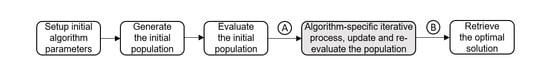
Metaheuristics are a special class of algorithms that can be used to solve search and optimization problems. As described in [34], they are approximate, usually non-deterministic methods that aim to search for solutions near the global optimum, exploring this space through a partly guided and partly random search. While the main disadvantage of metaheuristics is the uncertainty of reaching the global optimal solution, their advantages lie in not being problem-specific (allowing the flexibility of applying the same solving principle to several types of problems) and having intuitive mathematical models, borrowing concepts and approaches from the natural world, rather than from theoretical mathematical models. This contributes to their accessibility for a wider range of users. Most modern metaheuristics are population-based, starting from an initial group of solutions, called ‘population’, generated randomly, and refining it in an iterative process, according to a set of specific steps, until a stopping criterion is met. The performance of each individual from the population is assessed by computing its fitness function. The basic block diagram of a population-based metaheuristic algorithm (PMA) is depicted in Figure 1, where the steps common to all algorithms are represented with white boxes, and the part specific to each algorithm, delimited by symbols (A) and (B) is presented in gray.
The initial parameters are partially common to all algorithms, such as population size N or maximum number of iterations maxit, and partially specific to each algorithm, such as the mutation rate rmut for the Genetic Algorithm (GA) or inertia value w for the Particle Swarm Optimization (PSO). An individual from a population with N members, denoted in the following as
is encoded as a vector with length m, and element types and values dictated by the problem that needs to be solved. It usually represents an input parameter combination or a possible solution for the problem, which must satisfy all the constraints of the optimization model. The fitness evaluation of each population member requires the decoding of the information contained in the solution that it represents, solving the problem and evaluating the results. The optimality degree of the solution is assessed with the fitness function value associated to the respective population member. For a population with N members, Xi, i = 1, ..., N, N fitness functions will be computed and ranked.
The (A) to (B) section from Figure 1 consists of several steps, which describe each specific metaheuristic algorithm. While in the figures accompanying Section 2.1, Section 2.2, Section 2.3, Section 2.4 and Section 2.5 are presented all the details specific to each algorithm, delimited by (A) to (B), Table 2 summarizes their main steps, emphasizing their particularities.
Among the various metaheuristic algorithms available in the literature, those from Table 2 were chosen taking into account the following reasoning: the genetic algorithm and the particle swarm optimization are the best known and widely used metaheuristics, with numerous applications in power systems, which makes them a valid basis for comparison. The bat algorithm and the whale optimization algorithm are newer algorithms, previously used by the authors in solving similar optimization problems and shown to improve the quality of the results, compared with GA and PSO [35,36]. On the other hand, the sperm whale algorithm is a novelty in solving optimization problems in the power systems field. The results from the case study will show that the SWA outperforms the previous algorithms, making it a viable new alternative for solving optimization problems related to power systems applications.
The best-known PMAs are the genetic algorithm and the particle swarm optimization, which also describe two fundamental search principles used by metaheuristic algorithms: the evolutionary and performance-based patterns.
2.1. Genetic Algorithms
The Genetic Algorithm (GA), proposed in [37], is probably the best-known metaheuristic algorithm. In the GA, population members are named ‘chromosomes’, and their elements are ‘genes’. The search and optimization mechanisms use Darwinist natural evolution, based on perpetuation through genetic material exchange and mutation inside a population of same-species individuals, across a significant number of generations (iterations).
For finding new and improved solutions for an optimization problem, the GA relies on changing the population by using in each iteration the three main genetic operators (Figure 2):
- Selection: From the existing population, whole individuals are selected based on their performance, expressed by the fitness function. The better-adapted individuals are favored for surviving. In the standard GA, the population size is constant. Thus, the lesser adapted individuals, which are discarded, are replaced by clones of the survivors.
- Crossover: Pairs of parent chromosomes exchange a number of genes, the resulting offspring having new characteristics, possibly resulting in better solutions for the problem.
- Mutation: Randomly generated variations on gene values, resulting in chromosomes with minor structural changes, simulating genetic mutations of real living organisms.
Optionally, an elitist procedure can also be incorporated in the GA, which ensures the preservation of the best-found optimal solution and its fitness function across generations.
The literature offers a high variety of selection [38] and crossover [39] types, which together with the user-chosen crossover and mutation rates provide significant customization possibilities, making the GA a flexible problem-solving tool.
In this paper, the tournament selection method was used, which draws randomly p members from the existing population, out of which retains the best q, according to their fitness function. The procedure is repeated until a new population of size N is created.
The method of choice for the crossover operator was the uniform crossover, illustrated in Figure 3. Two parents are randomly chosen from the population and, for each gene, a random number is generated. The parents swap the genes only if the generated random number exceeds a customizable threshold tr.
2.2. Particle Swarm Optimization
On the other hand, the PSO algorithm [40] uses a different search method, based on variable travel speeds and position shifting in the search space. Each individual (‘particle’) from the population (‘swarm’) changes its speed in each iteration based on its current distance from two reference points: The best solution found so far by the swarm leader and the best position ever achieved by the particle itself. Compared with the GA, the PSO mechanism, presented in Figure 4, is very simple, requiring for each particle j, j = 1, ..., N, only the computation of its new speed and position:
followed by the update of each particle’s best position and the change of the leader position, if better solutions are found. The particle speeds are initialized with low random values, which would not influence the search direction.
In Equations (2) and (3), spj(it) and spj(it − 1) are the speed of particle xj (j = 1…N) in the previous (it − 1) and current (it) iteration, rnd1 and rnd2 are random vectors, x j,best(it) and x j,crt(it) are the best personal and the current position of particle xj, leader(it) is the position of the leader in iteration it, and xj(it) is the position of particle x in the current iteration. The factor w from Equation (2) is an inertia term, which decreases over the iteration count, larger initial values encouraging exploration, and smaller final values enabling the exploitation or local search around the best-known optimal solution.
It should be noted that while the GA explores the search space using crossover to make random changes of the information that is already present in the population, the mutation probability being much smaller, PSO changes randomly the speed of each particle element, moving it in the direction of the leader and personal best position.
The newer metaheuristic methods used in this paper, while sharing the natural inspiration of GA and PSO, combine elements found in the two algorithms and increase the number of input parameters and the complexity of their mathematical model in order to improve their optimization performance. They are the Bat Optimization Algorithm (BOA), Whale Optimization Algorithm (WOA) and Sperm-Whale Algorithm (SWA).
2.3. The Bat Optimization Algorithm
Bats hunt for prey using echolocation. In the initial search stage, they emit high amplitude/low frequency ultrasound impulses, with low emission rate (10–20 imp/sec), decoding in real time the reflected waves in order to identify the approximate position of the prey. When a potential target is identified, the bat increases the pulse rate up to 200 imp/sec, and the pulse frequency, which enables it to search accurately the space separating it from the prey, identifying the obstacles in its path and precisely locating the victim and its movement pattern.
The bat optimization algorithm [41] uses the PSO principle of changing the speed and position of the population members (here called ‘bats’), but the speed update formula is more elaborated, considering the principle of raising the signal frequency and pulse rate as the bats are getting close to the prey, i.e., to the optimal solution. The basic flowchart of a BOA iteration is depicted in Figure 5.
The bats’ speeds are initialized in the same manner as in the PSO algorithm but are accompanied by the initial signal amplitude, Aj, maximum pulse rate, rj,max and random pulse frequency fj ∈ [fmin, fmax], j = 1, ..., N.
In each iteration it, every bat from the population performs three operations:
- Frequency update:
- Speed update, with an equation inspired from (2):
- Position update, identical to the formulation from (3):
The BOA also includes a local search. The best individuals from the population are randomly moved in the search space, with
where is the average bat amplitude for iteration it and pp ∈ [–1, 1].
The new bat positions computed with Equations (4) to (7) are accepted in the population with random probability and only if the newly obtained position is better than the previous.
At the end of each iteration, if a bat improves its position, its signal amplitude is decreased:
and its pulse emission rate increases:
where α ∈ (0, 1) and γ > 0.
This behavior, much like the inertia term for PSO, increases the probability of performing local searches when the iteration count is nearing itmax.
2.4. The Whale Optimization Algorithm
The hunting behavior of humpback whales is the source of inspiration for the Whale Optimization Algorithm (WOA). The whales hunt in groups, and when they find their prey, consisting of schools of krill or small fish near the water surface, they attack it from below using two maneuvers: encircling and spiraling.
The WOA uses a population of vector solutions (‘whales’), which are hunting for prey independently, guiding their search by following a reference individual, usually their leader, i.e., the whale closest to the problem solution (‘food’), according to its fitness function.
During the algorithm, whales use initially encircling, then spiral attack, in the same way PSO and BOA use the broad exploration and the exploitation of the search space near the optimal solution.
In each iteration it, the encircling performed by each whale j from the population is described by [42]:
where
The coefficient a from equation (11) is a scalar value decreasing during the iterative from a positive value to 0. The (∙) sign denotes the element-by-element multiplying of vectors, and | |, an absolute value.
For the extreme values of a = 0 and a = 1, equations (10) to (12) show that position xj(it+1) will always lie between xj(it) and reference(it), thus moving any whale towards the reference solution used to guide the population. If values larger than 1 are given to a, factor A from (11) will also increase, moving the wales beyond the target and exploring a possibly uncharted portion of the search space.
If the reference position is reference(it) = leader(it), the leader from the current iteration, when A decreases, whales get closer to the leader, encircling the prey or the optimal solution. If another whale is used as reference, reference(it) = random(x(it)), the search will shift towards its path, simulating the exploration of the sea in search for food performed by real whales.
The spiral attack phase is described by an equation that combines oscillatory and exponentially variating components:
with
The initially large, then gradually decreasing values of a, so that first |A| > 1, then |A| < 1, |A| → 0, first move the whales away from the leader in exploration, then encourage encircling, followed by spiral attack. If p denotes a random number, the general equation for changing the position of a whale follows as:
The flowchart of a WOA iteration is presented in Figure 6.
WOA has two specific parameters that can be tuned for better performance: coefficient a from Equation (11) and constant b from (13).
2.5. The Sperm-Whale Algorithm
The search used by the SWA mimics the hunting behavior of sperm whales, which live alone or in small groups at the bottom of the sea and must come to the surface to hunt and breathe [43]. In each iteration, the population of the SWA is split into smaller search groups consisting in uniformly distributed better and worse adapted members (‘sperm whales’). Consequently, the search for the optimal solution occurs independently in each group. First, the sperm whales change their position from the bottom of the sea to the surface. This step is simulated only for the worst adapted member of the group, for which the opposite position is computed. The positions of the leader and of the worst individual in a group g, leader(g,it) and worst(g,it), are used to compute an in-between distance dist(g,it):
The reflex position of worst(g,it) is then computed with Equation (17).
The newly computed individual reflex(g,it) will replace worst(g,it) only if its fitness function is better. At the beginning of the iterative process, when the inertia w from Equation (16) is large, the individual will search beyond leader(g,it) (exploration phase, Figure 7a). As w decreases, the search will focus between worst(g,it) and leader(g,it), exploiting the search space around the known optimal solution (Figure 7b).
In the second stage, a Good Gang is formed within the group, gathering the best gg individuals ranked according to their fitness function. Every Good Gang member performs several local searches in which its elements k are displaced randomly, within a small radius r:
The original Good Gang members are replaced only if better sperm-whale positions are found during the local search.
Finally, the best Good Gang member from the group (the dominant sperm-whale) performs genetic crossover with all other group individuals. One of the two resulting children is chosen randomly to replace the worst of the two parents.
At the end of the iteration, the groups are reunited in the final population, which will repeat the search process until the stopping criterion of the algorithm is met. The basic flowchart of a SWA iteration is presented in Figure 8.
The SWA offers several tuning options for the user. The population size, number of search groups within the population, the inertia w and its decrement, the Good Gang size and number of local searches for its members, the local search radius r, and the crossover method can be adjusted for better performance.
3. The Implementation of the Optimal Reactive Compensation for Loss Minimization Problem
The five metaheuristic algorithms presented in the previous chapter were run in an implementation of the Optimal Capacitor Banks Allocation (OCBA) problem for active energy loss minimization. The approach used in this paper is stated as follows: Find the optimal buses in an EDN where capacitor banks (CB) should be installed and the amount of reactive load compensation in each bus, with the objective of operating the EDN with minimal active power and energy losses for the interval of a typical day. For an EDN with NN buses (nodes) and NB branches, the mathematical expression of the objective function of the OCBA problem was defined as:
The mathematical model of the fitness function considered the following constraints:
Cr1. The available CB stock cannot be exceeded:
Cr2. The compensation level in each bus cannot exceed the reactive bus load (avoid reversed reactive power flows):
Cr3. Branch current flows after compensation cannot exceed the branch rated current:
Cr4. Bus voltages after compensation cannot exceed the maximum allowed value:
In Equations (19) to (22), ΔP[%] is the percent active power loss in the EDN over 24 h, ΔPh is the active power loss in the EDN at hour h, NCBbus is the number of CBs installed in a generic bus; qCB is the reactive power rating of a CB, Qbus is the reactive load of a generic bus, stockCB is the CB stock; Ibr is the current flow on a generic branch br, Imax,br is the rated current of branch br, Ubus is the voltage of a generic bus after compensation, and Umax,bus is the maximum bus voltage allowed in a generic bus.
All the algorithms tested in the case study used the same solution encoding for their population members. They were generated as vectors of the type described by Equation (1), with integer numbers and length equal to the number of buses in which compensation was possible in the network. The significance of the value of a generic element represented the number of CBs placed in the bus to which it was designated. All the algorithms started in the first iteration with the same population, generated randomly but considering constraint Cr2 of maximum allowed number of CBs in each bus and Cr1, the maximum CB stock (Figure 9).
The fitness of the optimal solutions was assessed in all the algorithms using the objective function (19), which also considered the constraints from Equations (20) to (23). The methodology employed for calculating the fitness of each solution is described in Figure 10.
By applying any of the equations (2) to (18) or by genetic crossover and mutation, the changes undergone by population members can result in their invalidation because of
- Non-integer values, leading to invalid number of CBs installed in a bus;
- Values exceeding the interval [0, NCBbus] allowed by the constraint Cr2;
- Violation of constraint Cr1, by exceeding the available CB stock;
- Solutions otherwise valid but which lead to the violation of the constraints Cr3 or Cr4.
Thus, every newly generated population member, for each algorithm, must pass through a validation procedure before being allowed in the population created for the next iteration.
If constraint Cr1 is not satisfied, the solution is always discarded as unfeasible. If the constraint Cr2 is not fulfilled, the solution is modified by setting the unfeasible values to the nearest allowed value, using for each element xj from Figure 1 and Figure 9 the following correction:
For each population member, the active power losses used in equation (19) are computed with the Newton–Raphson load flow (LF) algorithm, which is slower, but generally considered more accurate than the branch-and-bound methods preferred in the analysis of distribution networks. The LF algorithm also provides the results required for checking the constraints Cr3 and Cr4, bus voltage and branch current flow limits. Prior to computing the LF, the compensation solution is simulated subtracting from the bus reactive loads the CB injection for each compensated bus, according to the population member/solution being tested.
4. Results
The OCBA problem was solved using the metaheuristics presented in Section 2, with the aim of comparing the performance of the newer algorithm designs, BOA, WOA, and SWA against the two well established methods, GA and PSO. For comparison purposes, all the algorithms had a common representation for the members of the population, illustrated in Figure 9, and the same fitness function, active power and energy loss minimization, computed with Equation (19) and subjected to the constraints given by Equations (20) to (23), Section 3. The initial parameters used for the algorithms are presented in Table 3.
Since for all algorithms there was no improvement for the optimal solution beyond generation 350, the graphical representations of the results will be limited to the first 360 generations.
Two test networks were used to validate the comparison: the smaller sized IEEE 33-bus MV radial voltage distribution system (Figure 11) and a larger 215-bus MV EDN from a residential area of a major city from Romania (Figure 12).
Synthetic data regarding the physical characteristics for the IEEE 33-bus system is given in Table 4. The system does not include MV/LV transformer data; thus, the active power losses computed by the algorithms do not include transformer losses. The extended data regarding branch characteristics (connecting buses, type line or transformer, electrical parameters resistance and reactance, maximum branch current) is provided in Appendix A, Table A1. For the active and reactive bus loads, the study uses a custom representation consisting of daily 24-h profiles, described below.
For this particular test system, the literature provides only a set of instantaneous active and reactive bus loads. In this paper, these values were used as reference, in conjunction with a set of typical load profiles (TLP) provided in the Supplementary Materials attached to the paper, to create 24-h profiles. The TLPs considered several types of loads, residential, industrial, and their distribution in the network is summarized in Table 5.
The second test system used in the case study is a much larger EDN, consisting of 135 MV buses to which 80 loads are connected through MV/LV transformers. For simplicity, the transformers are omitted in Figure 12, together with the corresponding 80 bus numbers for the transformer LV busbars (from 136 to 215). A summary of the transformer rated power, together with the feeder and bus general information, is given in Table 6. The electrical parameters of the branches are given in Appendix A, Table A2. For this network, the bus loads were also modelled as 24-h daily profiles, being measured by the smart metering infrastructure installed by the local distribution utility for a typical working day.
Because a 24-h voltage profile was not available for the 215-bus network, the voltage reference for the slack bus was recommended by the distribution utility at the value of 1.06 pu. For the IEEE 33-bus system, the setpoint was 1 pu (nominal voltage). The slack bus for both networks is bus 1, and all the other buses are modeled as PQ (consumer) buses.
4.1. Results for the IEEE 33-Bus System
The first step of the study was the choice of the maximum CB stock used for optimization. For this purpose, the load profile of the network for 24 h, given in Figure 13, was analyzed. Since the purpose was to test the performance of each algorithm, the CB stock was set at 70 × 7.5 kVar units, which would ensure a maximum of 525 kVar of VAR compensation, about half of the minimal value of the reactive load, occurring at night hours. In this way, the number of possible CB allocation variants is maximized, while reducing the investment cost.
The GA, PSO, BOA, WOA, and SWA were run using this CB stock, the initial parameters from Table 3, and the same initial population. The solution identified by each algorithm, compared with the reference case (no reactive power compensation), and their corresponding fitness functions (percent losses) are presented in Table 7. The first line of Table 7 also presents the maximum number of CBs that can be allocated in each bus, computed according to the minimal reactive power load, so that constraint Cr2 would be always fulfilled. The same results are displayed graphically in Figure 14. In Figure 15, the parallel evolution of the fitness function of each algorithm over the first 350 generations is presented, on a typical run, emphasizing the fact that the SWA and BOA obtain the solutions corresponding to the lowest loss values, followed by the PSO, GA, and BAT.
The results from Table 7 and Figure 14 show that the best fitness function values are obtained when maximum compensation is applied at buses 18 (feeder end), 29–32 (feeder end), and 12–14, while for other buses with compensation potential, such as 21–25, where the reactive load is high, no capacitor banks are allocated. All the algorithms use the entire CB stock available, with differences in the buses chosen for compensation and number of CBs allocated to each bus.
The results regarding the active power losses, for each hour and algorithm, compared with the reference case are plotted in Figure 16 and presented in Table 8. Table 9 gives the loss reduction in percent, against the reference case, for which the total values are represented in Figure 17. The loss reduction ranges between 6.55% and 16.78%, depending on the algorithm and network load. The improvement is higher in off-peak hours, and the best results are obtained with SWA (8.17% to 16.78%), with a global value of 10.51% over 24 h. PSO, WOA, and SWA are the closest to the optimal solution.
Compared with the reference case, the best compensation solution found by the SWA leads to a loss reduction of 726.73 kW for the analyzed day, which, if it is extrapolated for a year, amounts to 265.26 MW loss saving. The difference between SWA and the second best result, given by WOA, is of 6.25 kW per day or 2.28 MW for an entire year. As Figure 16 shows, SWA achieves these savings mainly during two hours, at 19.00 and 24.00.
Reactive power compensation with capacitor banks is mainly used in EDN for voltage profile improvement, where specific networks configurations and load patterns lead to high voltage drops along the feeders. In the case of the IEEE 33-bus system, the nominal voltage setting for the slack bus and the load profiles from Appendix A lead, in the reference case without compensation, to the voltage profile described by Figure 18.
The values show voltage drops that exceed the lower limit of –10% prescribed by the Romanian standards, in several buses located near the end of the main two supply paths, ending in buses 18 and 33. For bus 18, the voltage has the minimum value of 0.858 pu, at hours 19.00 and 20.00, while for bus 33, the minimum voltage is 0.882 pu, at hour 10.00.
The improvement of the voltages obtained hourly with each algorithm is depicted in Figure 19 for bus 18 and in Figure 20 for bus 33. The percent improvements over the reference values (no compensation) are given in Table 10 and Table 11, respectively. Again, the SWA gives the best results, with the maximum voltage improvement. The minimum reference voltage value of 0.858 pu in bus 18 (hour 10.00) is raised by 1.65%, to 0.872 pu. However, the voltages remain below the 0.9 pu minimum allowed limit, for 10 h from the 24-h analysis interval. Better voltage regulation can be possible using a larger CB stock or raising the voltage in the reference bus, by changing the HV/MV transformer tap position from the substation at bus 1.
The voltage improvements are smaller for bus 33, with a maximum of 1.28% with the SWA, but with three algorithms (SWA, PSO and WOA), the voltage levels are raised after compensation above the maximum –10% deviation allowed by the regulations during 7 h (8.00, 9.00, 12.00, 13.00, 18.00, 19.00, and 20.00), only two hours remaining below this threshold (10.00 and 11.00), as it can be seen in Figure 20.
4.2. Results for the 215-Bus Distribution Network
In this case, the CB stock used for compensation was chosen using the 24-h load profile of the network from Figure 21. In comparison with the IEEE 33-bus system, the minimum off-peak reactive load is reduced, while the number of buses available for compensation increases significantly, allowing a higher number of possible solutions. Thus, the CB stock was set at 90 units of 7.5 kVar each, providing a maximum of 675 kVar of reactive power. As the solutions from Figure 22 and Table 12 show, all the algorithms use the entire stock, with different bus allocation. The SWA provides the best solution (6.19% active power losses), followed by the PSO (6.21%). In Table 12, since the VAR compensation is performed at the LV side of the substation transformers, the bus numbers are given for both the MV buses denoted in Figure 12, and for their corresponding LV transformer busbars. In Figure 22, only the LV bus numbers are used, for better readability. Figure 23 presents the evolution of the fitness function of each metaheuristic algorithm over the first 360 generations, on a typical run.
For this network, as Figure 22 shows, the best two solutions (SWA, PSO) are mainly differentiated by the CB allocation at buses 151, LV side (28, MV side); 153 (31); 155 (34); 156 (35); and 157 (36), located at the beginning of the network, and having significant reactive power loads. This behavior is triggered by the use of the 90 CB stock, which is close to the maximum possible number of CBs that can be allocated for compensation, 107, and because of the sufficient stock, most of the buses can use the maximum possible CB allocation.
The comparison between the hourly active power losses computed by the Newton–Raphson algorithm for the reference case (no compensation) and the losses determined for each best compensation solution found by the metaheuristic algorithms is presented in Table 13 and Figure 24. Furthermore, Table 14 gives the percent reduction in losses obtained using the compensation solutions, while Figure 25 allows for an overview of the total losses obtained in each case, based on the values computed in Table 13.
The best CB allocation solution, obtained with the SWA, achieves a loss reduction of 833.91 kW or 10.36% for the entire network, in 24 h, which amounts to 304.38 MW in an entire year. The next best solution, found with the PSO algorithm, achieves only 816.58 kW (10.15%). The difference between the two solutions is of 17.33 kW in the analyzed day, or 6.32 MW in a year. The improvement over the IEEE 33-bus system regarding the loss reduction can be attributed to the presence of the MV/LV transformers.
The bus voltage levels for all 24 h and buses from the 215-bus network are presented in Figure 26. The length of the main feeder and the bus loadings lead to low voltage levels at the last buses on the main supply path, with values below the 0.9 pu limit at the LV side. At the MV side, the voltages are inside the allowed range, varying from 1.060 pu in the slack bus to 0.940 pu.
Figure 27 and Figure 28 depict the effect of VAR compensation on the voltages at bus 135 (MV) and 215 (LV). By allocating the available CB stock according to the solutions found by the five metaheuristic algorithms, the bus voltages increase with maximum 1.36%, as shown in Table 15 for bus 215 (LV). This increase is not sufficient for raising the lowest voltage values above the desired limit of 0.9 pu. Since the CB stock is near the maximum allowed reactive load compensation which fulfills constraint Cr2 specified by the optimization model, an alternative solution is to change the MV/LV transformer tap settings in the affected buses.
5. Discussions and Conclusions
The reactive power flow in the active electricity distribution networks has an important influence on the bus voltage level and the active power losses. Therefore, in order to control the reactive power absorbed by consumers, their consumption must be characterized by a power factor approximately equal to the neutral value (0.9 in Romania). Optimal allocation of reactive sources in the electricity distribution networks is made for power losses reduction, power factor correction and/or voltage profile improvement.
The optimization model considered in the paper has as main objective the optimal allocation of capacitor banks (CBs) in the medium voltage networks to minimize the power/energy losses, taking into account the technical restrictions imposed by the available CB stock, the compensation level in each bus, branch current flows, and bus voltages. This is very useful for distribution network operators that install now large amounts of capacitor banks (CB) in the distribution networks. In order to optimize the location of these CBs, the used test networks (the IEEE 33-bus system and a real 215-bus EDN from Romania) were modelled considering the MV lines, the MV/LV transformers from the electric distribution substations, where available, and the MV and LV buses. The different algorithms (Genetic Algorithm (GA), Particle Swarm Optimization (PSO), Bat Optimization Algorithm (BOA), Whale Optimization Algorithm (WOA) and Sperm-Whale Algorithm (SWA)) were tested to see which would be the best to solve the problem of capacitor bank allocation. The study, made using the IEEE 33-bus system, highlighted the fact that the SWA leads to the best results compared to the other algorithms. Compared with the reference case, the best compensation solution found by the SWA leads to a loss reduction of 726.73 kW for the analyzed day, which, if it is extrapolated for a year, amounts to 265.26 MW loss saving. The difference between SWA and the second best result, given by WOA, is of 6.25 kW per day or 2.28 MW for an entire year. In the case of the voltage level, an improvement was observed on the entire electricity distribution network, in all nodes, also obtained with the help of SWA. The minimum reference voltage value in bus 18 (the farthest node), at hour 10.00, was increased by 1.65%.
Moreover, the algorithms were tested in a real electricity distribution network (215-bus EDN) from Romania. The best CB allocation solution, obtained again with the SWA, achieves a loss reduction of 833.91 kW or 10.36% for the entire network, in 24 h, which amounts to 304.38 MW in an entire year. The next best solution, found with the PSO algorithm, achieves only 816.58 kW (10.15%). The difference between the two solutions is of 17.33 kW in the analyzed day, or 6.32 MW in a year. The solutions found led to an increase of the voltage in the farthest node (215) with maximum 1.36%.
Based on the obtained results, it can be affirmed that the use of capacitor banks is an easy solution to be implemented with technical and economic benefits to the electricity distribution networks that maximizes long-term return on investment as the network develops. An intelligent control of capacitor banks leads to improved energy efficiency and voltage level in the buses of electricity distribution networks, resulting in an increase in the percentage of energy delivered to consumers. Amongst the tested algorithms, the SWA finds the best compensation solutions, which can lead to significant additional loss savings and shorter investment recovery times.
Supplementary Materials
The following are available online at https://www.mdpi.com/1996-1073/12/22/4239/s1, file IEEE33_load_data.xls, active and reactive load profiles for the IEEE-33bus test system, and file EDN215_load_data.xls, active and reactive load profiles for the 215-bus distribution network.
Author Contributions
Conceptualization, O.I., B.-C.N. and G.G.; methodology, O.I. and G.G.; software, O.I. and B.-C.N.; validation, B.-C.N. and G.G.; formal analysis, M.G.; investigation, O.I. and B.-C.N.; data curation, B.-C.N.; writing—original draft preparation, O.I. and B.-C.N.; writing—B.-C.N., G.G. and M.G.; supervision, M.G.
Funding
This research received no external funding.
Conflicts of Interest
The authors declare no conflict of interest.
Appendix A

Table A1.
Branch parameters for the IEEE 33-bus system.
| Bus 1 | Bus 2 | Imax, A | Type1 | Resistance, Ω | Reactance, Ω |
|---|---|---|---|---|---|
| 1 | 2 | 420 | 1 | 0.092 | 0.047 |
| 2 | 3 | 420 | 1 | 0.493 | 0.251 |
| 3 | 4 | 420 | 1 | 0.366 | 0.186 |
| 4 | 5 | 420 | 1 | 0.381 | 0.194 |
| 5 | 6 | 420 | 1 | 0.819 | 0.707 |
| 6 | 7 | 420 | 1 | 0.187 | 0.619 |
| 7 | 8 | 420 | 1 | 0.711 | 0.235 |
| 8 | 9 | 420 | 1 | 1.03 | 0.74 |
| 9 | 10 | 420 | 1 | 1.044 | 0.74 |
| 10 | 11 | 420 | 1 | 0.197 | 0.065 |
| 11 | 12 | 420 | 1 | 0.374 | 0.124 |
| 12 | 13 | 420 | 1 | 1.468 | 1.155 |
| 13 | 14 | 420 | 1 | 0.542 | 0.713 |
| 14 | 15 | 420 | 1 | 0.591 | 0.526 |
| 15 | 16 | 420 | 1 | 0.746 | 0.545 |
| 16 | 17 | 420 | 1 | 1.289 | 1.721 |
| 17 | 18 | 420 | 1 | 0.732 | 0.574 |
| 19 | 20 | 420 | 1 | 1.504 | 1.356 |
| 2 | 19 | 420 | 1 | 0.164 | 0.157 |
| 20 | 21 | 420 | 1 | 0.41 | 0.478 |
| 21 | 22 | 420 | 1 | 0.709 | 0.937 |
| 23 | 24 | 420 | 1 | 0.898 | 0.709 |
| 24 | 25 | 420 | 1 | 0.896 | 0.701 |
| 26 | 27 | 420 | 1 | 0.284 | 0.145 |
| 27 | 28 | 420 | 1 | 1.059 | 0.934 |
| 28 | 29 | 420 | 1 | 0.804 | 0.701 |
| 29 | 30 | 420 | 1 | 0.508 | 0.259 |
| 3 | 23 | 420 | 1 | 0.451 | 0.308 |
| 30 | 31 | 420 | 1 | 0.975 | 0.963 |
| 31 | 32 | 420 | 1 | 0.311 | 0.362 |
| 32 | 33 | 420 | 1 | 0.341 | 0.53 |
| 6 | 26 | 420 | 1 | 0.203 | 0.103 |
1 Branch type can be 1—line; 2—transformer.
Table A2.
Branch parameters for the 215-bus distribution network.
| Bus 1 | Bus 2 | Imax, A | Type | Resistance, Ω | Reactance, Ω |
|---|---|---|---|---|---|
| 1 | 2 | 235 | 1 | 0.80625 | 0.314159 |
| 2 | 3 | 315 | 1 | 0.1051 | 0.061104 |
| 2 | 4 | 295 | 1 | 0.7701 | 0.358142 |
| 4 | 5 | 295 | 1 | 0.00154 | 0.000716 |
| 4 | 6 | 295 | 1 | 0.30804 | 0.143257 |
| 6 | 7 | 295 | 1 | 0.021306 | 0.009909 |
| 7 | 8 | 295 | 1 | 0.021306 | 0.009909 |
| 8 | 9 | 295 | 1 | 0.272102 | 0.126543 |
| 8 | 29 | 295 | 1 | 0.056474 | 0.026264 |
| 9 | 10 | 295 | 1 | 0.02567 | 0.011938 |
| 9 | 11 | 295 | 1 | 0.213061 | 0.099086 |
| 11 | 12 | 295 | 1 | 0.115515 | 0.053721 |
| 101 | 102 | 295 | 1 | 0.141185 | 0.065659 |
| 101 | 103 | 295 | 1 | 0.02567 | 0.011938 |
| 104 | 105 | 295 | 1 | 0.02567 | 0.011938 |
| 104 | 106 | 295 | 1 | 0.361947 | 0.168327 |
| 106 | 107 | 295 | 1 | 0.02567 | 0.011938 |
| 106 | 108 | 295 | 1 | 0.2567 | 0.119381 |
| 108 | 109 | 295 | 1 | 0.05134 | 0.023876 |
| 108 | 110 | 295 | 1 | 0.467194 | 0.217273 |
| 110 | 111 | 295 | 1 | 0.115515 | 0.053721 |
| 110 | 113 | 295 | 1 | 0.12835 | 0.05969 |
| 12 | 13 | 295 | 1 | 0.07701 | 0.035814 |
| 12 | 14 | 295 | 1 | 0.019253 | 0.008954 |
| 111 | 112 | 295 | 1 | 0.041072 | 0.019101 |
| 113 | 114 | 295 | 1 | 0.2567 | 0.119381 |
| 113 | 125 | 295 | 1 | 0.07701 | 0.035814 |
| 114 | 115 | 295 | 1 | 0.173273 | 0.080582 |
| 114 | 116 | 295 | 1 | 0.035938 | 0.016713 |
| 116 | 117 | 295 | 1 | 0.369648 | 0.171908 |
| 116 | 119 | 295 | 1 | 0.07701 | 0.035814 |
| 117 | 118 | 295 | 1 | 0.202793 | 0.094311 |
| 119 | 120 | 295 | 1 | 0.562173 | 0.261443 |
| 120 | 121 | 295 | 1 | 0.15402 | 0.071628 |
| 120 | 122 | 295 | 1 | 0.110381 | 0.051334 |
| 122 | 123 | 295 | 1 | 0.187391 | 0.087148 |
| 123 | 124 | 295 | 1 | 0.187391 | 0.087148 |
| 125 | 126 | 295 | 1 | 0.038505 | 0.017907 |
| 125 | 127 | 295 | 1 | 0.169422 | 0.078791 |
| 127 | 128 | 295 | 1 | 0.02567 | 0.011938 |
| 127 | 129 | 295 | 1 | 0.064175 | 0.029845 |
| 129 | 130 | 295 | 1 | 0.20536 | 0.095504 |
| 129 | 131 | 295 | 1 | 0.361947 | 0.168327 |
| 14 | 15 | 295 | 1 | 0.097546 | 0.045365 |
| 14 | 22 | 295 | 1 | 0.035938 | 0.016713 |
| 131 | 132 | 295 | 1 | 0.120649 | 0.056109 |
| 131 | 133 | 295 | 1 | 0.17969 | 0.083566 |
| 131 | 134 | 295 | 1 | 0.2567 | 0.119381 |
| 134 | 135 | 295 | 1 | 0.033371 | 0.015519 |
| 15 | 16 | 295 | 1 | 0.15402 | 0.071628 |
| 16 | 17 | 295 | 1 | 0.15402 | 0.071628 |
| 16 | 18 | 295 | 1 | 0.019253 | 0.008954 |
| 18 | 19 | 295 | 1 | 0.17969 | 0.083566 |
| 18 | 20 | 295 | 1 | 0.019253 | 0.008954 |
| 20 | 21 | 295 | 1 | 0.02567 | 0.011938 |
| 22 | 23 | 295 | 1 | 0.351679 | 0.163551 |
| 22 | 24 | 295 | 1 | 0.248999 | 0.115799 |
| 24 | 25 | 295 | 1 | 0.23103 | 0.107442 |
| 25 | 26 | 295 | 1 | 0.071876 | 0.033427 |
| 25 | 27 | 295 | 1 | 0.392751 | 0.182652 |
| 27 | 28 | 295 | 1 | 0.10268 | 0.047752 |
| 29 | 30 | 295 | 1 | 0.038505 | 0.017907 |
| 30 | 31 | 295 | 1 | 0.071876 | 0.033427 |
| 30 | 37 | 295 | 1 | 0.056474 | 0.026264 |
| 31 | 32 | 295 | 1 | 0.123216 | 0.057303 |
| 32 | 33 | 295 | 1 | 0.087278 | 0.040589 |
| 33 | 34 | 295 | 1 | 0.192525 | 0.089535 |
| 33 | 35 | 295 | 1 | 0.071876 | 0.033427 |
| 35 | 36 | 295 | 1 | 0.351679 | 0.163551 |
| 37 | 38 | 295 | 1 | 0.10268 | 0.047752 |
| 37 | 40 | 295 | 1 | 0.318308 | 0.148032 |
| 39 | 38 | 309 | 1 | 0.46244 | 0.268858 |
| 40 | 41 | 295 | 1 | 0.41072 | 0.191009 |
| 40 | 43 | 295 | 1 | 0.403019 | 0.187427 |
| 42 | 41 | 295 | 1 | 0.12835 | 0.05969 |
| 43 | 44 | 295 | 1 | 0.084711 | 0.039396 |
| 44 | 45 | 295 | 1 | 0.33371 | 0.155195 |
| 44 | 47 | 295 | 1 | 0.189958 | 0.088342 |
| 45 | 46 | 295 | 1 | 0.02567 | 0.011938 |
| 47 | 48 | 295 | 1 | 0.238731 | 0.111024 |
| 47 | 56 | 295 | 1 | 0.338844 | 0.157582 |
| 48 | 49 | 295 | 1 | 0.17969 | 0.083566 |
| 48 | 50 | 295 | 1 | 0.238731 | 0.111024 |
| 50 | 51 | 295 | 1 | 0.288788 | 0.134303 |
| 50 | 52 | 295 | 1 | 0.040045 | 0.018623 |
| 52 | 53 | 295 | 1 | 0.07701 | 0.035814 |
| 52 | 54 | 295 | 1 | 0.10268 | 0.047752 |
| 54 | 55 | 295 | 1 | 0.23103 | 0.107442 |
| 56 | 57 | 295 | 1 | 0.05134 | 0.023876 |
| 56 | 59 | 295 | 1 | 0.659719 | 0.306808 |
| 57 | 58 | 295 | 1 | 0.10268 | 0.047752 |
| 59 | 60 | 295 | 1 | 0.043639 | 0.020295 |
| 59 | 66 | 295 | 1 | 0.084711 | 0.039396 |
| 60 | 61 | 295 | 1 | 0.02567 | 0.011938 |
| 60 | 62 | 295 | 1 | 0.074443 | 0.03462 |
| 62 | 63 | 295 | 1 | 0.441524 | 0.205335 |
| 62 | 64 | 295 | 1 | 0.028237 | 0.013132 |
| 64 | 65 | 295 | 1 | 0.17969 | 0.083566 |
| 66 | 67 | 295 | 1 | 0.17969 | 0.083566 |
| 66 | 73 | 295 | 1 | 0.467194 | 0.217273 |
| 67 | 68 | 295 | 1 | 0.10268 | 0.047752 |
| 67 | 69 | 295 | 1 | 0.120649 | 0.056109 |
| 69 | 70 | 295 | 1 | 0.02567 | 0.011938 |
| 69 | 71 | 295 | 1 | 0.210494 | 0.097892 |
| 71 | 72 | 295 | 1 | 0.02567 | 0.011938 |
| 73 | 74 | 295 | 1 | 0.02567 | 0.011938 |
| 73 | 75 | 295 | 1 | 0.467194 | 0.217273 |
| 75 | 76 | 295 | 1 | 0.64175 | 0.298451 |
| 75 | 78 | 295 | 1 | 0.021306 | 0.009909 |
| 76 | 77 | 295 | 1 | 0.30804 | 0.143257 |
| 78 | 79 | 295 | 1 | 0.15402 | 0.071628 |
| 78 | 80 | 295 | 1 | 0.084711 | 0.039396 |
| 80 | 81 | 295 | 1 | 0.02567 | 0.011938 |
| 80 | 82 | 295 | 1 | 0.12835 | 0.05969 |
| 82 | 83 | 295 | 1 | 0.10268 | 0.047752 |
| 82 | 84 | 295 | 1 | 0.189958 | 0.088342 |
| 84 | 85 | 295 | 1 | 0.23103 | 0.107442 |
| 84 | 86 | 295 | 1 | 0.2567 | 0.119381 |
| 86 | 87 | 295 | 1 | 0.05134 | 0.023876 |
| 86 | 88 | 295 | 1 | 0.5134 | 0.238761 |
| 88 | 89 | 295 | 1 | 0.07701 | 0.035814 |
| 88 | 92 | 295 | 1 | 0.084711 | 0.039396 |
| 89 | 90 | 295 | 1 | 0.02567 | 0.011938 |
| 89 | 91 | 295 | 1 | 0.02567 | 0.011938 |
| 92 | 93 | 295 | 1 | 0.5134 | 0.238761 |
| 93 | 94 | 295 | 1 | 0.02567 | 0.011938 |
| 93 | 95 | 295 | 1 | 0.084711 | 0.039396 |
| 95 | 96 | 295 | 1 | 0.07701 | 0.035814 |
| 95 | 98 | 295 | 1 | 0.12835 | 0.05969 |
| 96 | 97 | 295 | 1 | 0.053907 | 0.02507 |
| 98 | 99 | 295 | 1 | 0.084711 | 0.039396 |
| 98 | 100 | 295 | 1 | 0.064175 | 0.029845 |
| 100 | 101 | 295 | 1 | 0.07701 | 0.035814 |
| 100 | 104 | 295 | 1 | 0.12835 | 0.05969 |
| 2 | 136 | 1000 | 2 | 0.06 | 0.082 |
| 3 | 137 | 1000 | 2 | 0.011 | 0.037 |
| 5 | 138 | 1000 | 2 | 0.011 | 0.037 |
| 6 | 139 | 1000 | 2 | 0.011 | 0.037 |
| 7 | 140 | 1000 | 2 | 0.011 | 0.037 |
| 10 | 141 | 1000 | 2 | 0.019 | 0.036 |
| 11 | 142 | 1000 | 2 | 0.06 | 0.082 |
| 102 | 195 | 1000 | 2 | 0.04 | 0.05 |
| 103 | 196 | 1000 | 2 | 0.06 | 0.082 |
| 105 | 197 | 1000 | 2 | 0.011 | 0.037 |
| 107 | 198 | 1000 | 2 | 0.06 | 0.082 |
| 109 | 199 | 1000 | 2 | 0.011 | 0.037 |
| 111 | 200 | 1000 | 2 | 0.006 | 0.023 |
| 112 | 201 | 1000 | 2 | 0.011 | 0.037 |
| 115 | 202 | 1000 | 2 | 0.06 | 0.082 |
| 117 | 203 | 1000 | 2 | 0.06 | 0.082 |
| 118 | 204 | 1000 | 2 | 0.06 | 0.082 |
| 119 | 205 | 1000 | 2 | 0.06 | 0.082 |
| 13 | 143 | 1000 | 2 | 0.019 | 0.036 |
| 121 | 206 | 1000 | 2 | 0.011 | 0.037 |
| 122 | 207 | 1000 | 2 | 0.06 | 0.082 |
| 123 | 208 | 1000 | 2 | 0.06 | 0.082 |
| 124 | 209 | 1000 | 2 | 0.019 | 0.036 |
| 126 | 210 | 1000 | 2 | 0.06 | 0.082 |
| 128 | 211 | 1000 | 2 | 0.019 | 0.036 |
| 130 | 212 | 1000 | 2 | 0.019 | 0.036 |
| 132 | 213 | 1000 | 2 | 0.006 | 0.023 |
| 133 | 214 | 1000 | 2 | 0.06 | 0.082 |
| 135 | 215 | 1000 | 2 | 0.019 | 0.036 |
| 15 | 144 | 1000 | 2 | 0.06 | 0.082 |
| 17 | 145 | 1000 | 2 | 0.04 | 0.05 |
| 19 | 146 | 1000 | 2 | 0.06 | 0.082 |
| 21 | 147 | 1000 | 2 | 0.011 | 0.037 |
| 23 | 148 | 1000 | 2 | 0.06 | 0.082 |
| 24 | 149 | 1000 | 2 | 0.06 | 0.082 |
| 26 | 150 | 1000 | 2 | 0.06 | 0.082 |
| 28 | 151 | 1000 | 2 | 0.019 | 0.036 |
| 29 | 152 | 1000 | 2 | 0.06 | 0.082 |
| 31 | 153 | 1000 | 2 | 0.04 | 0.05 |
| 32 | 154 | 1000 | 2 | 0.019 | 0.036 |
| 34 | 155 | 1000 | 2 | 0.019 | 0.036 |
| 35 | 156 | 1000 | 2 | 0.011 | 0.037 |
| 36 | 157 | 1000 | 2 | 0.04 | 0.05 |
| 38 | 158 | 1000 | 2 | 0.011 | 0.037 |
| 39 | 159 | 1000 | 2 | 0.019 | 0.036 |
| 40 | 160 | 1000 | 2 | 0.019 | 0.036 |
| 41 | 161 | 1000 | 2 | 0.04 | 0.05 |
| 42 | 162 | 1000 | 2 | 0.06 | 0.082 |
| 43 | 163 | 1000 | 2 | 0.019 | 0.036 |
| 45 | 164 | 1000 | 2 | 0.006 | 0.023 |
| 46 | 165 | 1000 | 2 | 0.06 | 0.082 |
| 49 | 166 | 1000 | 2 | 0.06 | 0.082 |
| 51 | 167 | 1000 | 2 | 0.06 | 0.082 |
| 53 | 168 | 1000 | 2 | 0.04 | 0.05 |
| 55 | 169 | 1000 | 2 | 0.04 | 0.05 |
| 57 | 170 | 1000 | 2 | 0.019 | 0.036 |
| 58 | 171 | 1000 | 2 | 0.06 | 0.082 |
| 61 | 172 | 1000 | 2 | 0.011 | 0.037 |
| 63 | 173 | 1000 | 2 | 0.06 | 0.082 |
| 64 | 174 | 1000 | 2 | 0.06 | 0.082 |
| 65 | 175 | 1000 | 2 | 0.06 | 0.082 |
| 68 | 176 | 1000 | 2 | 0.06 | 0.082 |
| 70 | 177 | 1000 | 2 | 0.04 | 0.05 |
| 71 | 178 | 1000 | 2 | 0.06 | 0.082 |
| 72 | 179 | 1000 | 2 | 0.06 | 0.082 |
| 74 | 180 | 1000 | 2 | 0.06 | 0.082 |
| 76 | 181 | 1000 | 2 | 0.06 | 0.082 |
| 77 | 182 | 1000 | 2 | 0.04 | 0.05 |
| 79 | 183 | 1000 | 2 | 0.04 | 0.05 |
| 81 | 184 | 1000 | 2 | 0.06 | 0.082 |
| 83 | 185 | 1000 | 2 | 0.04 | 0.05 |
| 85 | 186 | 1000 | 2 | 0.04 | 0.05 |
| 87 | 187 | 1000 | 2 | 0.011 | 0.037 |
| 90 | 188 | 1000 | 2 | 0.011 | 0.037 |
| 91 | 189 | 1000 | 2 | 0.011 | 0.037 |
| 92 | 190 | 1000 | 2 | 0.06 | 0.082 |
| 94 | 191 | 1000 | 2 | 0.04 | 0.05 |
| 96 | 192 | 1000 | 2 | 0.019 | 0.036 |
| 97 | 193 | 1000 | 2 | 0.04 | 0.05 |
| 99 | 194 | 1000 | 2 | 0.019 | 0.036 |
References
- T&D World Magazine. Capacitor Bank Control Adapts to Evolving Challenges of Smart Grid. Available online: https://www.tdworld.com/test-monitor-amp-control/capacitor-bank-control-adapts-evolving-challenges-smart-grid (accessed on 15 July 2019).
- Cooper Power Series. Smart Grid Ready Capacitor Bank Control Delivers Automation and Efficiency. Available online: https://www.eaton.com/content/dam/eaton/products/utility-and-grid-solutions/grid-automation-systems/capacitor-bank-control/cbc-8000-capacitor-bank-control/cbc-8000-capacitor-bank-pa916001en.pdf (accessed on 15 July 2019).
- Hogan, P.M.; Rettkowski, J.D.; Bala, J.L. Optimal capacitor placement using branch and bound. In Proceedings of the 37th Annual North American Power Symposium, Ames, IA, USA, 25 October 2005; pp. 84–89. [Google Scholar]
- Grainger, J.; Lee, S. Optimum Size and Location of Shunt Capacitors for Reduction of Losses on Distribution Feeders. IEEE Trans. Power Appar. Syst. 1981, 3, 1105–1118. [Google Scholar] [CrossRef]
- Muthukumar, K.; Jayalalitha, S. Optimal placement and sizing of distributed generators and shunt capacitors for power loss minimization in radial distribution networks using hybrid heuristic search optimization technique. Int. J. Electr. Power Energy Syst. 2016, 78, 299–319. [Google Scholar] [CrossRef]
- Segura, S.; Romero, R.; Rider, M.J. Efficient heuristic algorithm used for optimal capacitor placement in distribution systems. Int. J. Electr. Power Energy Syst. 2010, 32, 71–78. [Google Scholar] [CrossRef]
- Biagio, M.A.; Coelho, M.A.; Franco, P.E.C. Heuristic for solving capacitor allocation problems in electric energy radial distribution networks. Pesquisa Oper. 2012, 32, 121–138. [Google Scholar] [CrossRef] [Green Version]
- Bakker, E.; Deljou, V.; Rahmani, J. Optimal Placement of Capacitor Bank in Reorganized Distribution Networks Using Genetic Algorithm. Int. J. Comp. App. Techn. Res. (IJCATR) 2019, 8, 2319–8656. [Google Scholar] [CrossRef]
- Ozgonenel, O.; Karagol, S. A novel generation and capacitor integration technique for today’s distribution systems, Turk. J. Elec. Eng. Comp. Sci. 2017, 25, 2434–2443. [Google Scholar] [CrossRef]
- Villa-Acevedo, W.; López-Lezama, J.; Valencia-Velásquez, J. A novel constraint handling approach for the optimal reactive power dispatch problem. Energies 2018, 11, 2352. [Google Scholar] [CrossRef]
- Rahmani-andebili, M. Simultaneous placement of DG and capacitor in distribution network. Electr. Power Syst. Res. 2016, 131, 1–10. [Google Scholar] [CrossRef]
- Bhattacharya, S.K.; Goswami, S.K. A new fuzzy based solution of the capacitor placement problem in radial distribution system. Expert Syst. Appl. 2009, 36, 4207–4212. [Google Scholar] [CrossRef]
- Kumar, M.; Nallagownden, P.; Elamvazuthi, I. Optimal Placement and Sizing of Renewable Distributed Generations and Capacitor Banks into Radial Distribution Systems. Energies 2017, 10, 811. [Google Scholar] [CrossRef]
- Zeinalzadeh, A.; Mohammadi, Y.; Moradi, M.H. Optimal multi objective placement and sizing of multiple DGs and shunt capacitor banks simultaneously considering load uncertainty via MOPSO approach. Int. J. Electr. Power Energy Syst. 2015, 67, 336–349. [Google Scholar] [CrossRef]
- Sharaf, A.M.; El-Gammal, A.A. Optimal selection of capacitors in distribution networks for voltage stabilization and loss reduction. In Proceedings of the 2010 IEEE Electrical Power & Energy Conference, Halifax, NS, Canada, 25–27 August 2010; pp. 1–5. [Google Scholar]
- Díaz, P.; Pérez-Cisneros, M.; Cuevas, E.; Avalos, O.; Gálvez, J.; Hinojosa, S.; Zaldivar, D. An improved crow search algorithm applied to energy problems. Energies 2018, 11, 571. [Google Scholar] [CrossRef]
- Montazeri, M.; Askarzadeh, A. Capacitor placement in radial distribution networks based on identification of high potential busses. Int. Trans. Elec. Energy Syst. 2019, 29, e2754. [Google Scholar] [CrossRef]
- Jiang, F.; Zhang, Y.; Zhang, Y.; Liu, X.; Chen, C. An Adaptive Particle Swarm Optimization Algorithm Based on Guiding Strategy and Its Application in Reactive Power Optimization. Energies 2019, 12, 1690. [Google Scholar] [CrossRef]
- Elsheikh, A.; Helmy, Y.; Abouelseoud, Y.; Elsherif, A. Optimal capacitor placement and sizing in radial electric power systems. Alex. Eng. J. 2014, 53, 809–816. [Google Scholar] [CrossRef] [Green Version]
- Arulraj, R.; Kumarappan, N. Optimal economic-driven planning of multiple DG and capacitor in distribution network considering different compensation coefficients in feeder’s failure rate evaluation. Eng. Sci. Technol. Int. J. 2019, 22, 67–77. [Google Scholar] [CrossRef]
- Sahli, Z.; Hamouda, A.; Bekrar, A.; Trentesaux, D. Reactive Power Dispatch Optimization with Voltage Profile Improvement Using an Efficient Hybrid Algorithm. Energies 2018, 11, 2134. [Google Scholar] [CrossRef]
- Abdelaziz, A.Y.; Ali, E.S.; Elazim, S.A. Flower pollination algorithm and loss sensitivity factors for optimal sizing and placement of capacitors in radial distribution systems. Int. J. Electr. Power Energy Syst. 2016, 78, 207–214. [Google Scholar] [CrossRef]
- Tamilselvan, V.; Jayabarathi, T.; Raghunathan, T.; Yang, X.S. Optimal capacitor placement in radial distribution systems using flower pollination algorithm. Alex. Eng. J. 2018, 57, 2775–2786. [Google Scholar] [CrossRef]
- Ali, E.S.; Elazim, S.A.; Abdelaziz, A.Y. Improved Harmony Algorithm for optimal locations and sizing of capacitors in radial distribution systems. Int. J. Electr. Power Energy Syst. 2016, 79, 275–284. [Google Scholar] [CrossRef]
- Devabalaji, K.R.; Ravi, K.; Kothari, D.P. Optimal location and sizing of capacitor placement in radial distribution system using bacterial foraging optimization algorithm. Int. J. Electr. Power Energy Syst. 2015, 71, 383–390. [Google Scholar] [CrossRef]
- Kishore, C.; Ghosh, S.; Karar, V. Symmetric fuzzy logic and IBFOA solutions for optimal position and rating of capacitors allocated to radial distribution networks. Energies 2018, 11, 766. [Google Scholar] [CrossRef]
- Khodabakhshian, A.; Andishgar, M.H. Simultaneous placement and sizing of DGs and shunt capacitors in distribution systems by using IMDE algorithm. Int. J. Electr. Power Energy Syst. 2016, 82, 599–607. [Google Scholar] [CrossRef]
- Dixit, M.; Kundu, P.; Jariwala, H.R. Incorporation of distributed generation and shunt capacitor in radial distribution system for techno-economic benefits. Eng. Sci. Technol. Int. J. 2017, 20, 482–493. [Google Scholar] [CrossRef]
- Mouassa, S.; Bouktir, T.; Salhi, A. Ant lion optimizer for solving optimal reactive power dispatch problem in power systems. Eng. Sci. Technol. Int. J. 2017, 20, 885–895. [Google Scholar] [CrossRef]
- Baysal, Y.A.; Altas, İ.H. Power quality improvement via optimal capacitor placement in electrical distribution systems using symbiotic organisms search algorithm. Mugla J. Sci. Technol. 2017, 3, 64–68. [Google Scholar] [CrossRef]
- Helmy, W.; Abbas, M.A.E. Optimal sizing of capacitor-bank types in the low voltage distribution networks using JAYA optimization. In Proceedings of the 9th International Renewable Energy Congress (IREC), Hammamet, Tunisia, 20–22 March 2018; pp. 1–5. [Google Scholar]
- Sultana, S.; Roy, P.K. Capacitor Placement in Radial Distribution System Using Oppositional Cuckoo Optimization Algorithm. Int. J. Swarm Intel. Res. (IJSIR) 2018, 9, 64–95. [Google Scholar] [CrossRef]
- Neagu, B.C.; Ivanov, O.; Gavrilaş, M. A comprehensive solution for optimal capacitor allocation problem in real distribution networks. In Proceedings of the Conference on Electromechanical and Power System (SIELMEN), Iaşi, Romania, 11–13 October 2017; pp. 565–570. [Google Scholar]
- Blum, C.; Roli, A. Metaheuristics in Combinatorial Optimization: Overview and Conceptual Comparison. ACM Comp. Surv. 2003, 35, 268–308. [Google Scholar] [CrossRef]
- Neagu, B.C.; Ivanov, O.; Georgescu, G. Reactive Power Compensation in Distribution Networks Using the Bat Algorithm. In Proceedings of the International Conference and Exposition on Electrical and Power Engineering, Iasi, Romania, 20–22 October 2016; pp. 711–714. [Google Scholar]
- Neagu, B.C.; Ivanov, O.; Gavrilas, M. Voltage profile improvement in distribution networks using the whale optimization algorithm. In Proceedings of the International Conference on Electronics, Computers and Artificial Intelligence (ECAI 2017), Targoviste, Romania, 29 June–1 July 2017. [Google Scholar]
- Holland, J.H. Adaptation in Natural and Artificial Systems: An Introductory Analysis with Applications to Biology, Control and Artificial Systems; University of Michigan Press: Ann Arbor, MI, USA, 1975. [Google Scholar]
- Jebari, K. Selection Methods for Genetic Algorithms. Int. J. Emerg. Sci. 2013, 3, 333–344. [Google Scholar]
- Umbarkar, A.J.; Sheth, P.D. Crossover Operators in Genetic Algorithms: A Review. ICTACT J. Soft Comput. 2015, 6, 1083–1092. [Google Scholar]
- Kennedy, J.; Eberhart, R.C. Particle Swarm Optimization. In Proceedings of the ICNN’95—International Conference on Neural Networks, Perth, WA, Australia, 27 November–1 December 1995; IEEE: Piscataway, NJ, USA, 1995. [Google Scholar]
- Yang, X.S. A New Metaheuristic Bat-Inspired Algorithm. In Nature Inspired Cooperative Strategies for Optimization (NISCO 2010); Cruz, C., González, J.R., Krasnogor, N., Pelta, D.A., Terrazas, G., Eds.; Springer: Berlin, Germany, 2010; pp. 65–74. [Google Scholar] [Green Version]
- Mirjalili, S.; Lewis, A. The Whale Optimization Algorithm. Adv. Eng. Soft. 2016, 95, 51–67. [Google Scholar] [CrossRef]
- Ebrahimi, A.; Khamehchi, E. Sperm whale algorithm: An effective metaheuristic algorithm for production optimization problems. J. Nat. Gas. Sci. Eng. 2016, 29, 211–222. [Google Scholar] [CrossRef]
Figure 1.
The basic flowchart of a population-based metaheuristic algorithm.

Figure 2.
The flowchart of a GA iteration.

Figure 3.
The uniform crossover.

Figure 4.
The flowchart of a PSO iteration.

Figure 5.
The flowchart of a BOA iteration.

Figure 6.
The flowchart of a WOA iteration.

Figure 7.
Reflex search in the SWA algorithm: (a) exploration, (b) exploitation.

Figure 8.
The flowchart of a SWA iteration.

Figure 9.
The encoding of the solutions used by the OCBA problem.

Figure 10.
Fitness computation and solution validation for the OCBA problem.

Figure 11.
The IEEE 33-bus test system.

Figure 12.
The residential 215-bus EDN.

Figure 13.
The active and reactive load profiles of the IEEE 33-bus test system—hourly values.

Figure 14.
The number of CBs allocated in the buses of the IEEE 33-bus system by each algorithm.

Figure 15.
The fitness of the optimal solution found by the metaheuristic algorithms after 360 iterations, for the IEEE 33-bus system.
Figure 15.
The fitness of the optimal solution found by the metaheuristic algorithms after 360 iterations, for the IEEE 33-bus system.

Figure 16.
Hourly active power losses in the IEEE 33-bus system, for each algorithm.

Figure 17.
The total active power loss reduction in the IEEE 33-bus system, in kW, for each algorithm.
Figure 17.
The total active power loss reduction in the IEEE 33-bus system, in kW, for each algorithm.

Figure 18.
The bus voltages in the IEEE 33-bus system without compensation, for each hour from the analyzed day.
Figure 18.
The bus voltages in the IEEE 33-bus system without compensation, for each hour from the analyzed day.

Figure 19.
Voltage improvement after compensation for bus 18, the IEEE 33-bus system.

Figure 20.
Voltage improvement after compensation for bus 33, the IEEE 33-bus system.

Figure 21.
The active and reactive load profiles of the 215-bus network—hourly values.

Figure 22.
The number of CBs allocated in the buses of the 215-bus network by each algorithm: (a)—buses 136-175, (b)—buses 176-215.
Figure 22.
The number of CBs allocated in the buses of the 215-bus network by each algorithm: (a)—buses 136-175, (b)—buses 176-215.

Figure 23.
The fitness of the optimal solution found by the metaheuristic algorithms after 360 iterations, for the 215-bus network.
Figure 23.
The fitness of the optimal solution found by the metaheuristic algorithms after 360 iterations, for the 215-bus network.

Figure 24.
Hourly active power losses in the IEEE 33-bus system, for each algorithm.

Figure 25.
The total active power loss reduction in the 215-bus network, in kW, for each algorithm.

Figure 26.
The bus voltages in the 215-bus network without compensation, for each hour from the analyzed day.
Figure 26.
The bus voltages in the 215-bus network without compensation, for each hour from the analyzed day.

Figure 27.
Voltage improvement after compensation for bus 135, medium voltage, the 215-bus network.

Figure 28.
Voltage improvement after compensation for bus 215, low voltage, the 215-bus network.

Table 1.
Literature review regarding the capacitor allocation problem based on artificial intelligence.
Table 1.
Literature review regarding the capacitor allocation problem based on artificial intelligence.
| Objective Function | Constraints | Test Network | References | ||||||||
|---|---|---|---|---|---|---|---|---|---|---|---|
| C1 | C2 | C3 | C4 | C5 | C6 | C7 | C8 | C9 | |||
| OF1 | X | X | - | - | - | - | - | - | - | 38 bus—Roy–Billinton Test System | [8] |
| X | - | X | - | X | X | - | - | - | IEEE 30, 57, 118 and 300 bus | [10,27,29] | |
| X | - | X | - | X | - | - | - | - | IEEE 33 bus | [13] | |
| X | X | X | X | - | - | - | - | - | IEEE 33 and 94 bus | [14,15] | |
| X | X | X | - | X | X | - | - | - | IEEE 30 bus | [21] | |
| X | X | X | - | X | - | - | - | - | IEEE 33 and 85 bus | [25,28] | |
| X | X | X | X | X | - | - | - | - | IEEE 33 and 119 bus | [5] | |
| OF2 | X | - | - | - | - | - | - | - | - | IEEE 10, 23 and 34 bus | [12] |
| X | - | X | - | X | - | - | - | - | IEEE 22, 69, 85 and 141 bus | [32] | |
| OF3 | X | - | X | - | X | X | - | - | - | IEEE 30, 57, 118 and 300 bus | [10,27] |
| X | X | X | - | X | X | - | - | - | IEEE 30 bus | [21] | |
| OF4 | X | - | X | - | - | - | X | - | X | IEEE 10, 33 and 69 bus | [16,17,22,26] |
| X | - | X | - | - | - | - | X | - | IEEE 10, 15 and 34 bus | [19] | |
| X | - | X | - | - | - | - | - | - | IEEE 30 and 85 bus | [20] | |
| X | - | X | - | - | - | - | - | - | IEEE 33, 34, 69 and 85 bus | [23,27] | |
| X | - | X | - | X | - | X | - | X | IEEE 85 and 118 bus | [24] | |
| OF5 | X | - | - | - | X | - | - | - | - | IEEE 28-bus | [11] |
| X | - | - | - | - | - | - | - | - | IEEE 9-bus | [30] | |
| OF6 | X | - | X | - | - | X | X | - | - | IEEE 30 bus | [18] |
| X | - | X | - | X | X | X | - | - | IEEE 30, 57 and 118 bus | [27] | |
| X | - | X | - | X | - | - | - | - | IEEE 30, 118 and 300 bus | [29] | |
Table 2.
The metaheuristic algorithms used in the paper for solving the OCBA problem.
| Algorithm | Main Steps |
|---|---|
| Genetic Algorithm (GA) | Selection, crossover, mutation, using the entire population |
| Particle Swarm Optimization (PSO) | Speed and position update, using the entire population, and exploration followed by exploitation of the search space |
| The Bat Optimization Algorithm (BOA) | Speed and position update, frequency adaptation, and local search in each iteration, using the entire population, exploration followed by exploitation |
| The Whale Optimization Algorithm (WOA) | Continuous choice between three search methods: exploration, encircling, and spiral attack, using the entire population |
| The Sperm Whale Algorithm (SWA) | Population divided in subgroups that perform the search independently, using dominant crossover in each subgroup |
Table 3.
The initial parameters used for the metaheuristic algorithms.
| Common Parameters for All the Algorithms: |
|---|
| Population size: 40, Number of generations: 500 |
| GA |
| Selection method: tournament—keep best 2 from a random draw of 4 |
| Crossover method: uniform at threshold 0.5 |
| Mutation: random |
| Crossover and mutation rates: 0.9/0.1 |
| PSO |
| Inertia: 0.9 decreasing to 0.4, linear descent |
| BOA |
| Initial amplitude: 1 |
| Initial pulse emission rate: 0.3 |
| Amplitude attenuation rate: 0.7 |
| Pulse emission increase rate: 0.3 |
| Pulse frequency domain: [–0.9, 1.2] |
| Number of bats used for local search: dynamic. If a randomly generated number is greater than the bat’s pulse emission rate, the bat is selected for local search in the current iteration. |
| WOA |
| Coefficient a: decreasing from 3 to 0, linear descent |
| Coefficient l: random |
| Coefficient b: 1 |
| SWA |
| Number of search groups: 4 |
| Good Gang size: half of the search group size, rounded to the nearest integer |
| Number of searches performed by each Good Gang member: 10 |
| Local search radius: 1 |
| Crossover type: uniform |
Table 4.
The physical characteristics of the IEEE 33-bus system.
| Number of Buses | Transformer Rated Power/Number | Feeder Type | Feeder Cross-Section (mm2) | Total Length(km) |
|---|---|---|---|---|
| 12.66 kV: 33 | None | Unknown(1) | Unknown(1) | Unknown(1) |
(1) Only the total resistance and reactance is known for each branch
Table 5.
The TLP categories used for the IEEE 33 -bus system and their bus distribution.
| TLP Category | Bus |
|---|---|
| Residential | 4, 5, 6, 7, 8, 9, 10, 11, 12, 13 14, 15, 16, 17, 18 |
| Industry | 2, 3, 19, 20, 21, 22, 23, 24, 25 |
| Commercial | 26, 27, 28, 29, 30, 31, 32, 33 |
Table 6.
The physical characteristics of the 215-bus EDN.
| Number of Buses | Transformer Rated Power/Number | Feeder Type | Feeder Cross-Section (mm2) | Total Length (km) |
|---|---|---|---|---|
| 20 kV: 135 (1–135) 0.4 kV: 80 (136–215) | 63 kVA: 33; 100 kVA: 14 160 kVA: 15, 250 kVA: 15 400 kVA: 3 | Cable | 3 × 95 3 × 120 3 × 150 | 2.5 84.45 3.2 |
Table 7.
The OCBA solutions found by the metaheuristic algorithms for the IEEE 33-bus system.
| Bus | 2 | 3 | 4 | 5 | 6 | 7 | 8 | 9 | 10 | 11 | 12 | 13 | 14 | 15 | 16 | 17 | 18 | |
|---|---|---|---|---|---|---|---|---|---|---|---|---|---|---|---|---|---|---|
| CB limit | 3 | 2 | 4 | 0 | 0 | 6 | 3 | 1 | 4 | 0 | 6 | 4 | 4 | 0 | 0 | 0 | 14 | |
| Reference | 0 | 0 | 0 | 0 | 0 | 0 | 0 | 0 | 0 | 0 | 0 | 0 | 0 | 0 | 0 | 0 | 0 | |
| GA | 1 | 1 | 1 | 0 | 0 | 1 | 1 | 1 | 2 | 0 | 5 | 1 | 2 | 0 | 0 | 0 | 13 | |
| PSO | 0 | 0 | 0 | 0 | 0 | 4 | 0 | 1 | 0 | 0 | 0 | 4 | 4 | 0 | 0 | 0 | 14 | |
| BAT | 0 | 2 | 4 | 0 | 0 | 3 | 1 | 1 | 1 | 0 | 6 | 4 | 3 | 0 | 0 | 0 | 2 | |
| WOA | 0 | 0 | 0 | 0 | 0 | 0 | 0 | 1 | 0 | 0 | 1 | 4 | 4 | 0 | 0 | 0 | 14 | |
| SWA | 0 | 0 | 0 | 0 | 0 | 0 | 0 | 0 | 0 | 0 | 4 | 4 | 4 | 0 | 0 | 0 | 14 | |
| Bus | 19 | 20 | 21 | 22 | 23 | 24 | 25 | 26 | 27 | 28 | 29 | 30 | 31 | 32 | 33 | CB Used | Fitness | |
| CB limit | 6 | 1 | 17 | 2 | 3 | 7 | 5 | 0 | 0 | 0 | 3 | 39 | 4 | 5 | 0 | 143 | N/A | |
| Reference | 0 | 0 | 0 | 0 | 0 | 0 | 0 | 0 | 0 | 0 | 0 | 0 | 0 | 0 | 0 | 0 | 5.482 | |
| GA | 1 | 1 | 1 | 1 | 1 | 1 | 1 | 0 | 0 | 0 | 1 | 27 | 4 | 2 | 0 | 70 | 4.982 | |
| PSO | 0 | 1 | 0 | 0 | 0 | 0 | 0 | 0 | 0 | 0 | 3 | 39 | 0 | 0 | 0 | 70 | 4.947 | |
| BAT | 0 | 1 | 0 | 1 | 3 | 7 | 2 | 0 | 0 | 0 | 2 | 24 | 2 | 1 | 0 | 70 | 5.038 | |
| WOA | 0 | 1 | 0 | 0 | 0 | 0 | 0 | 0 | 0 | 0 | 0 | 39 | 1 | 5 | 0 | 70 | 4.939 | |
| SWA | 0 | 0 | 0 | 0 | 0 | 0 | 0 | 0 | 0 | 0 | 0 | 35 | 4 | 5 | 0 | 70 | 4.934 | |
Table 8.
Hourly and total active power losses in the IEEE 33-bus system, in kW, for each algorithm.
| Hour | Ref. | BAT | GA | PSO | WOA | SWA |
|---|---|---|---|---|---|---|
| h01 | 140.04 | 122.53 | 120.22 | 118.98 | 118.74 | 118.51 |
| h02 | 128.61 | 111.53 | 109.32 | 108.14 | 107.93 | 107.70 |
| h03 | 122.58 | 105.89 | 103.74 | 102.65 | 102.45 | 102.22 |
| h04 | 119.17 | 102.76 | 100.65 | 99.59 | 99.39 | 99.17 |
| h05 | 118.50 | 102.35 | 100.31 | 99.31 | 99.13 | 98.90 |
| h06 | 128.54 | 112.25 | 110.25 | 109.23 | 109.04 | 108.82 |
| h07 | 205.62 | 184.05 | 181.30 | 179.43 | 178.99 | 178.75 |
| h08 | 314.56 | 287.82 | 284.37 | 281.89 | 281.25 | 280.98 |
| h09 | 374.57 | 345.89 | 342.50 | 340.05 | 339.35 | 339.12 |
| h10 | 448.92 | 416.40 | 412.92 | 410.21 | 409.41 | 409.15 |
| h11 | 462.22 | 427.75 | 424.10 | 421.26 | 420.40 | 420.17 |
| h12 | 404.06 | 373.11 | 370.05 | 367.81 | 367.11 | 366.87 |
| h13 | 408.02 | 377.17 | 373.94 | 371.64 | 370.97 | 370.72 |
| h14 | 364.61 | 335.05 | 331.31 | 328.94 | 328.27 | 328.03 |
| h15 | 324.39 | 296.90 | 293.33 | 291.25 | 290.70 | 290.45 |
| h16 | 277.75 | 254.32 | 251.42 | 250.06 | 249.70 | 249.46 |
| h17 | 298.98 | 275.44 | 272.52 | 271.10 | 270.71 | 270.50 |
| h18 | 421.48 | 391.95 | 388.02 | 385.68 | 385.03 | 384.78 |
| h19 | 466.73 | 436.14 | 431.94 | 429.53 | 428.93 | 428.60 |
| h20 | 458.26 | 427.14 | 422.83 | 420.32 | 419.70 | 419.36 |
| h21 | 329.63 | 302.53 | 298.48 | 295.98 | 295.44 | 295.03 |
| h22 | 273.68 | 248.43 | 244.68 | 242.37 | 241.88 | 241.51 |
| h23 | 187.07 | 167.53 | 164.73 | 163.25 | 162.98 | 162.67 |
| h24 | 139.61 | 123.09 | 120.90 | 119.80 | 119.60 | 119.37 |
| total | 6917.59 | 6328.03 | 6253.83 | 6208.47 | 6197.11 | 6190.86 |
Table 9.
Hourly and total power loss reduction in the IEEE 33-bus system, in %, for each algorithm.
| Hour | BAT | GA | PSO | WOA | SWA |
|---|---|---|---|---|---|
| h01 | 12.50 | 14.15 | 15.03 | 15.21 | 15.37 |
| h02 | 13.28 | 15.00 | 15.91 | 16.08 | 16.26 |
| h03 | 13.62 | 15.37 | 16.26 | 16.42 | 16.61 |
| h04 | 13.77 | 15.54 | 16.43 | 16.60 | 16.78 |
| h05 | 13.62 | 15.35 | 16.19 | 16.35 | 16.54 |
| h06 | 12.67 | 14.22 | 15.02 | 15.17 | 15.34 |
| h07 | 10.49 | 11.83 | 12.74 | 12.95 | 13.06 |
| h08 | 8.50 | 9.60 | 10.39 | 10.59 | 10.67 |
| h09 | 7.66 | 8.56 | 9.22 | 9.40 | 9.47 |
| h10 | 7.24 | 8.02 | 8.62 | 8.80 | 8.86 |
| h11 | 7.46 | 8.25 | 8.86 | 9.05 | 9.10 |
| h12 | 7.66 | 8.42 | 8.97 | 9.15 | 9.20 |
| h13 | 7.56 | 8.35 | 8.92 | 9.08 | 9.14 |
| h14 | 8.11 | 9.13 | 9.78 | 9.97 | 10.03 |
| h15 | 8.47 | 9.57 | 10.21 | 10.38 | 10.46 |
| h16 | 8.44 | 9.48 | 9.97 | 10.10 | 10.18 |
| h17 | 7.87 | 8.85 | 9.32 | 9.46 | 9.53 |
| h18 | 7.00 | 7.94 | 8.49 | 8.65 | 8.71 |
| h19 | 6.55 | 7.46 | 7.97 | 8.10 | 8.17 |
| h20 | 6.79 | 7.73 | 8.28 | 8.41 | 8.49 |
| h21 | 8.22 | 9.45 | 10.21 | 10.37 | 10.50 |
| h22 | 9.23 | 10.60 | 11.44 | 11.62 | 11.76 |
| h23 | 10.45 | 11.94 | 12.73 | 12.88 | 13.04 |
| h24 | 11.83 | 13.40 | 14.19 | 14.33 | 14.49 |
| total | 8.52 | 9.60 | 10.25 | 10.42 | 10.51 |
Table 10.
Hourly reference voltage values for bus 18 and percent improvements after compensation, the IEEE 33-bus test system.
Table 10.
Hourly reference voltage values for bus 18 and percent improvements after compensation, the IEEE 33-bus test system.
| Hour | Voltage, pu | Improvement, % | ||||
|---|---|---|---|---|---|---|
| Ref. | BAT | GA | PSO | WOA | SWA | |
| h01 | 0.914 | 0.82 | 1.26 | 1.38 | 1.38 | 1.42 |
| h02 | 0.919 | 0.81 | 1.25 | 1.37 | 1.37 | 1.41 |
| h03 | 0.921 | 0.80 | 1.24 | 1.36 | 1.36 | 1.40 |
| h04 | 0.922 | 0.80 | 1.23 | 1.36 | 1.36 | 1.40 |
| h05 | 0.922 | 0.80 | 1.23 | 1.36 | 1.36 | 1.40 |
| h06 | 0.919 | 0.80 | 1.24 | 1.36 | 1.36 | 1.40 |
| h07 | 0.905 | 0.84 | 1.29 | 1.42 | 1.42 | 1.46 |
| h08 | 0.888 | 0.88 | 1.35 | 1.48 | 1.48 | 1.53 |
| h09 | 0.886 | 0.88 | 1.36 | 1.49 | 1.49 | 1.54 |
| h10 | 0.879 | 0.90 | 1.38 | 1.52 | 1.52 | 1.56 |
| h11 | 0.878 | 0.91 | 1.39 | 1.53 | 1.53 | 1.57 |
| h12 | 0.882 | 0.89 | 1.37 | 1.50 | 1.50 | 1.55 |
| h13 | 0.882 | 0.89 | 1.37 | 1.51 | 1.51 | 1.55 |
| h14 | 0.885 | 0.89 | 1.36 | 1.50 | 1.50 | 1.54 |
| h15 | 0.890 | 0.88 | 1.35 | 1.48 | 1.48 | 1.52 |
| h16 | 0.895 | 0.86 | 1.32 | 1.45 | 1.45 | 1.50 |
| h17 | 0.892 | 0.86 | 1.33 | 1.46 | 1.46 | 1.51 |
| h18 | 0.870 | 0.92 | 1.41 | 1.55 | 1.55 | 1.60 |
| h19 | 0.858 | 0.95 | 1.45 | 1.60 | 1.60 | 1.65 |
| h20 | 0.858 | 0.95 | 1.45 | 1.60 | 1.60 | 1.65 |
| h21 | 0.869 | 0.92 | 1.42 | 1.55 | 1.56 | 1.60 |
| h22 | 0.882 | 0.89 | 1.37 | 1.51 | 1.51 | 1.55 |
| h23 | 0.898 | 0.85 | 1.31 | 1.44 | 1.44 | 1.48 |
| h24 | 0.913 | 0.82 | 1.26 | 1.38 | 1.39 | 1.43 |
| minimum value, pu | 0.858 | |||||
| max. improvement, % | 0.95 | 1.45 | 1.60 | 1.60 | 1.65 | |
Table 11.
Hourly reference voltage values for bus 33 and percent improvements after compensation, the IEEE 33-bus test system.
Table 11.
Hourly reference voltage values for bus 33 and percent improvements after compensation, the IEEE 33-bus test system.
| Hour | Voltage, pu | Improvement, % | ||||
|---|---|---|---|---|---|---|
| Reference | BAT | GA | PSO | WOA | SWA | |
| h01 | 0.935 | 0.78 | 0.91 | 1.02 | 1.10 | 1.11 |
| h02 | 0.937 | 0.77 | 0.90 | 1.01 | 1.09 | 1.10 |
| h03 | 0.939 | 0.77 | 0.90 | 1.01 | 1.09 | 1.10 |
| h04 | 0.939 | 0.77 | 0.90 | 1.01 | 1.09 | 1.10 |
| h05 | 0.940 | 0.77 | 0.90 | 1.01 | 1.08 | 1.10 |
| h06 | 0.938 | 0.77 | 0.90 | 1.01 | 1.09 | 1.10 |
| h07 | 0.915 | 0.82 | 0.96 | 1.08 | 1.16 | 1.17 |
| h08 | 0.896 | 0.86 | 1.01 | 1.14 | 1.22 | 1.24 |
| h09 | 0.890 | 0.88 | 1.02 | 1.15 | 1.24 | 1.25 |
| h10 | 0.882 | 0.90 | 1.05 | 1.18 | 1.27 | 1.28 |
| h11 | 0.883 | 0.90 | 1.05 | 1.18 | 1.27 | 1.28 |
| h12 | 0.895 | 0.87 | 1.01 | 1.14 | 1.23 | 1.24 |
| h13 | 0.895 | 0.87 | 1.01 | 1.14 | 1.23 | 1.24 |
| h14 | 0.899 | 0.86 | 1.00 | 1.13 | 1.22 | 1.23 |
| h15 | 0.908 | 0.84 | 0.98 | 1.10 | 1.19 | 1.20 |
| h16 | 0.921 | 0.81 | 0.94 | 1.06 | 1.14 | 1.15 |
| h17 | 0.916 | 0.82 | 0.96 | 1.07 | 1.16 | 1.17 |
| h18 | 0.894 | 0.87 | 1.02 | 1.14 | 1.23 | 1.24 |
| h19 | 0.890 | 0.88 | 1.03 | 1.15 | 1.24 | 1.26 |
| h20 | 0.890 | 0.88 | 1.03 | 1.15 | 1.24 | 1.26 |
| h21 | 0.900 | 0.85 | 1.00 | 1.12 | 1.21 | 1.22 |
| h22 | 0.908 | 0.84 | 0.98 | 1.10 | 1.19 | 1.20 |
| h23 | 0.927 | 0.79 | 0.93 | 1.04 | 1.12 | 1.14 |
| h24 | 0.937 | 0.77 | 0.90 | 1.01 | 1.09 | 1.11 |
| minimum value, p.u. | 0.882 | |||||
| max. improvement, % | 0.90 | 1.05 | 1.18 | 1.27 | 1.28 | |
Table 12.
The OCBA solutions found by the metaheuristic algorithms for the 215-bus network.
| MV Bus | 2 | 3 | 5 | 6 | 7 | 10 | 11 | 13 | 15 | 17 | 19 | 21 | 23 | 24 | 26 | 28 | 29 | 31 | 32 | 34 | 35 |
|---|---|---|---|---|---|---|---|---|---|---|---|---|---|---|---|---|---|---|---|---|---|
| LV Bus | 136 | 137 | 138 | 139 | 140 | 141 | 142 | 143 | 144 | 145 | 146 | 147 | 148 | 149 | 150 | 151 | 152 | 153 | 154 | 155 | 156 |
| bus limit | 0 | 5 | 3 | 0 | 1 | 1 | 0 | 2 | 2 | 3 | 1 | 3 | 0 | 0 | 0 | 4 | 1 | 2 | 1 | 2 | 4 |
| reference | 0 | 0 | 0 | 0 | 0 | 0 | 0 | 0 | 0 | 0 | 0 | 0 | 0 | 0 | 0 | 0 | 0 | 0 | 0 | 0 | 0 |
| GA | 0 | 3 | 2 | 0 | 1 | 1 | 0 | 1 | 1 | 3 | 1 | 1 | 0 | 0 | 0 | 4 | 1 | 2 | 1 | 1 | 3 |
| PSO | 0 | 5 | 0 | 0 | 1 | 1 | 0 | 1 | 2 | 3 | 1 | 0 | 0 | 0 | 0 | 4 | 1 | 1 | 1 | 2 | 0 |
| BAT | 0 | 0 | 3 | 0 | 1 | 1 | 0 | 1 | 2 | 0 | 1 | 3 | 0 | 0 | 0 | 4 | 1 | 1 | 1 | 2 | 4 |
| WOA | 0 | 2 | 3 | 0 | 1 | 1 | 0 | 2 | 2 | 1 | 1 | 1 | 0 | 0 | 0 | 2 | 1 | 1 | 1 | 2 | 4 |
| SWA | 0 | 5 | 0 | 0 | 0 | 1 | 0 | 0 | 2 | 3 | 1 | 0 | 0 | 0 | 0 | 3 | 1 | 2 | 0 | 1 | 0 |
| MV Bus | 36 | 38 | 39 | 40 | 41 | 42 | 43 | 45 | 46 | 49 | 51 | 53 | 55 | 57 | 58 | 61 | 63 | 64 | 65 | 68 | 70 |
| LV Bus | 157 | 158 | 159 | 160 | 161 | 162 | 163 | 164 | 165 | 166 | 167 | 168 | 169 | 170 | 171 | 172 | 173 | 174 | 175 | 176 | 177 |
| bus limit | 2 | 1 | 0 | 1 | 0 | 1 | 0 | 5 | 0 | 1 | 0 | 2 | 2 | 1 | 1 | 2 | 0 | 1 | 1 | 1 | 1 |
| reference | 0 | 0 | 0 | 0 | 0 | 0 | 0 | 0 | 0 | 0 | 0 | 0 | 0 | 0 | 0 | 0 | 0 | 0 | 0 | 0 | 0 |
| GA | 1 | 1 | 0 | 1 | 0 | 1 | 0 | 5 | 0 | 1 | 0 | 2 | 2 | 1 | 1 | 2 | 0 | 1 | 1 | 1 | 1 |
| PSO | 1 | 1 | 0 | 1 | 0 | 1 | 0 | 5 | 0 | 1 | 0 | 0 | 2 | 1 | 1 | 2 | 0 | 1 | 1 | 1 | 1 |
| BAT | 1 | 1 | 0 | 1 | 0 | 1 | 0 | 5 | 0 | 1 | 0 | 2 | 2 | 1 | 1 | 2 | 0 | 1 | 1 | 1 | 1 |
| WOA | 1 | 1 | 0 | 1 | 0 | 1 | 0 | 5 | 0 | 1 | 0 | 1 | 1 | 1 | 1 | 2 | 0 | 1 | 1 | 1 | 1 |
| SWA | 2 | 0 | 0 | 1 | 0 | 1 | 0 | 5 | 0 | 1 | 0 | 2 | 2 | 1 | 1 | 2 | 0 | 1 | 1 | 1 | 1 |
| MV Bus | 71 | 72 | 74 | 76 | 77 | 79 | 81 | 83 | 85 | 87 | 90 | 91 | 92 | 94 | 96 | 97 | 99 | 102 | 103 | 105 | 107 |
| LV Bus | 178 | 179 | 180 | 181 | 182 | 183 | 184 | 185 | 186 | 187 | 188 | 189 | 190 | 191 | 192 | 193 | 194 | 195 | 196 | 197 | 198 |
| bus limit | 1 | 1 | 1 | 0 | 1 | 2 | 0 | 3 | 1 | 2 | 1 | 3 | 1 | 1 | 0 | 1 | 0 | 0 | 0 | 4 | 0 |
| reference | 0 | 0 | 0 | 0 | 0 | 0 | 0 | 0 | 0 | 0 | 0 | 0 | 0 | 0 | 0 | 0 | 0 | 0 | 0 | 0 | 0 |
| GA | 1 | 1 | 1 | 0 | 1 | 2 | 0 | 2 | 1 | 2 | 1 | 3 | 1 | 1 | 0 | 1 | 0 | 0 | 0 | 3 | 0 |
| PSO | 1 | 1 | 1 | 0 | 1 | 2 | 0 | 3 | 1 | 2 | 1 | 3 | 1 | 1 | 0 | 1 | 0 | 0 | 0 | 4 | 0 |
| BAT | 1 | 1 | 1 | 0 | 1 | 1 | 0 | 1 | 1 | 1 | 1 | 3 | 1 | 1 | 0 | 1 | 0 | 0 | 0 | 3 | 0 |
| WOA | 1 | 1 | 1 | 0 | 1 | 1 | 0 | 1 | 1 | 1 | 1 | 3 | 1 | 1 | 0 | 1 | 0 | 0 | 0 | 4 | 0 |
| SWA | 1 | 1 | 1 | 0 | 1 | 2 | 0 | 3 | 1 | 2 | 1 | 3 | 1 | 1 | 0 | 1 | 0 | 0 | 0 | 4 | 0 |
| MV Bus | 109 | 111 | 112 | 115 | 117 | 118 | 119 | 121 | 122 | 123 | 124 | 126 | 128 | 130 | 132 | 133 | 135 | ||||
| LV Bus | 199 | 200 | 201 | 202 | 203 | 204 | 205 | 206 | 207 | 208 | 209 | 210 | 211 | 212 | 213 | 214 | 215 | CB Used | Fitness | ||
| bus limit | 1 | 3 | 1 | 1 | 1 | 0 | 0 | 2 | 0 | 1 | 4 | 0 | 2 | 2 | 4 | 1 | 3 | 107 | |||
| reference | 0 | 0 | 0 | 0 | 0 | 0 | 0 | 0 | 0 | 0 | 0 | 0 | 0 | 0 | 0 | 0 | 0 | 0 | 6.8578 | ||
| GA | 1 | 2 | 1 | 1 | 1 | 0 | 0 | 2 | 0 | 1 | 4 | 0 | 1 | 2 | 4 | 1 | 0 | 90 | 6.2385 | ||
| PSO | 1 | 3 | 1 | 1 | 1 | 0 | 0 | 2 | 0 | 1 | 4 | 0 | 0 | 2 | 4 | 1 | 3 | 90 | 6.2050 | ||
| BAT | 1 | 3 | 1 | 1 | 1 | 0 | 0 | 1 | 0 | 1 | 4 | 0 | 2 | 2 | 4 | 1 | 3 | 90 | 6.2278 | ||
| WOA | 1 | 3 | 1 | 1 | 1 | 0 | 0 | 2 | 0 | 1 | 4 | 0 | 2 | 2 | 4 | 1 | 3 | 90 | 6.2175 | ||
| SWA | 1 | 3 | 1 | 1 | 1 | 0 | 0 | 2 | 0 | 1 | 4 | 0 | 2 | 2 | 4 | 1 | 3 | 90 | 6.1910 | ||
Table 13.
Hourly and total active power losses in the 215-bus network, in kW, for each algorithm.
| Hour | Ref. | BAT | GA | PSO | WOA | SWA |
|---|---|---|---|---|---|---|
| h01 | 67.331 | 55.673 | 55.609 | 55.539 | 55.583 | 55.305 |
| h02 | 56.182 | 45.636 | 45.575 | 45.517 | 45.541 | 45.319 |
| h03 | 53.214 | 43.113 | 43.053 | 43.000 | 43.016 | 42.817 |
| h04 | 58.190 | 47.878 | 47.818 | 47.762 | 47.782 | 47.572 |
| h05 | 90.377 | 77.534 | 77.467 | 77.382 | 77.446 | 77.109 |
| h06 | 147.228 | 131.143 | 131.068 | 130.941 | 131.065 | 130.562 |
| h07 | 245.758 | 223.025 | 223.059 | 222.583 | 222.867 | 222.029 |
| h08 | 290.292 | 262.257 | 262.479 | 261.527 | 261.962 | 260.864 |
| h09 | 303.227 | 270.552 | 271.077 | 269.405 | 270.026 | 268.696 |
| h10 | 296.025 | 261.012 | 261.713 | 259.595 | 260.336 | 258.874 |
| h11 | 354.181 | 312.943 | 313.922 | 311.078 | 312.050 | 310.247 |
| h12 | 363.306 | 320.607 | 321.658 | 318.606 | 319.647 | 317.753 |
| h13 | 352.690 | 310.099 | 311.147 | 308.090 | 309.134 | 307.242 |
| h14 | 350.992 | 308.310 | 309.373 | 306.281 | 307.332 | 305.437 |
| h15 | 394.674 | 349.439 | 350.570 | 347.313 | 348.428 | 346.400 |
| h16 | 393.582 | 349.764 | 350.799 | 347.811 | 348.843 | 346.908 |
| h17 | 505.757 | 458.845 | 459.845 | 456.827 | 457.938 | 455.824 |
| h18 | 741.209 | 680.993 | 682.464 | 678.467 | 679.882 | 677.100 |
| h19 | 892.805 | 825.937 | 827.555 | 823.210 | 824.773 | 821.637 |
| h20 | 795.742 | 736.564 | 737.748 | 734.379 | 735.670 | 732.945 |
| h21 | 672.197 | 623.613 | 624.385 | 621.999 | 622.971 | 620.808 |
| h22 | 304.238 | 280.233 | 280.128 | 279.887 | 280.171 | 279.245 |
| h23 | 194.076 | 175.399 | 175.315 | 175.153 | 175.327 | 174.688 |
| h24 | 122.607 | 107.163 | 107.100 | 106.949 | 107.055 | 106.594 |
| total | 8045.88 | 7257.73 | 7270.93 | 7229.30 | 7244.84 | 7211.97 |
Table 14.
Hourly and total power loss reduction in the 215-bus network, in %, for each algorithm.
| Hour | BAT | GA | PSO | WOA | SWA |
|---|---|---|---|---|---|
| h01 | 17.31 | 17.41 | 17.51 | 17.45 | 17.86 |
| h02 | 18.77 | 18.88 | 18.98 | 18.94 | 19.33 |
| h03 | 18.98 | 19.09 | 19.19 | 19.16 | 19.54 |
| h04 | 17.72 | 17.82 | 17.92 | 17.89 | 18.25 |
| h05 | 14.21 | 14.28 | 14.38 | 14.31 | 14.68 |
| h06 | 10.92 | 10.98 | 11.06 | 10.98 | 11.32 |
| h07 | 9.25 | 9.24 | 9.43 | 9.31 | 9.66 |
| h08 | 9.66 | 9.58 | 9.91 | 9.76 | 10.14 |
| h09 | 10.78 | 10.60 | 11.15 | 10.95 | 11.39 |
| h10 | 11.83 | 11.59 | 12.31 | 12.06 | 12.55 |
| h11 | 11.64 | 11.37 | 12.17 | 11.90 | 12.40 |
| h12 | 11.75 | 11.46 | 12.30 | 12.02 | 12.54 |
| h13 | 12.08 | 11.78 | 12.65 | 12.35 | 12.89 |
| h14 | 12.16 | 11.86 | 12.74 | 12.44 | 12.98 |
| h15 | 11.46 | 11.17 | 12.00 | 11.72 | 12.23 |
| h16 | 11.13 | 10.87 | 11.63 | 11.37 | 11.86 |
| h17 | 9.28 | 9.08 | 9.67 | 9.45 | 9.87 |
| h18 | 8.12 | 7.93 | 8.46 | 8.27 | 8.65 |
| h19 | 7.49 | 7.31 | 7.80 | 7.62 | 7.97 |
| h20 | 7.44 | 7.29 | 7.71 | 7.55 | 7.89 |
| h21 | 7.23 | 7.11 | 7.47 | 7.32 | 7.64 |
| h22 | 7.89 | 7.92 | 8.00 | 7.91 | 8.22 |
| h23 | 9.62 | 9.67 | 9.75 | 9.66 | 9.99 |
| h24 | 12.60 | 12.65 | 12.77 | 12.68 | 13.06 |
| total | 9.80 | 9.63 | 10.15 | 9.96 | 10.36 |
Table 15.
Hourly reference voltage values for bus 215 and percent improvements after compensation, the 215-bus network.
Table 15.
Hourly reference voltage values for bus 215 and percent improvements after compensation, the 215-bus network.
| Hour | Voltage, pu | Improvement, % | ||||
|---|---|---|---|---|---|---|
| Ref. | BAT | GA | PSO | WOA | SWA | |
| h01 | 1.019 | 0.86 | 0.36 | 0.86 | 0.87 | 0.88 |
| h02 | 1.022 | 0.85 | 0.35 | 0.86 | 0.86 | 0.87 |
| h03 | 1.022 | 0.85 | 0.35 | 0.86 | 0.86 | 0.87 |
| h04 | 1.021 | 0.86 | 0.35 | 0.86 | 0.86 | 0.87 |
| h05 | 1.014 | 0.87 | 0.36 | 0.87 | 0.88 | 0.89 |
| h06 | 1.004 | 0.89 | 0.37 | 0.89 | 0.90 | 0.91 |
| h07 | 0.983 | 0.94 | 0.39 | 0.94 | 0.95 | 0.96 |
| h08 | 0.965 | 0.99 | 0.41 | 0.99 | 0.99 | 1.01 |
| h09 | 0.948 | 1.04 | 0.43 | 1.04 | 1.04 | 1.06 |
| h10 | 0.940 | 1.06 | 0.45 | 1.07 | 1.07 | 1.09 |
| h11 | 0.922 | 1.12 | 0.47 | 1.13 | 1.13 | 1.15 |
| h12 | 0.917 | 1.14 | 0.48 | 1.15 | 1.15 | 1.16 |
| h13 | 0.918 | 1.14 | 0.48 | 1.14 | 1.15 | 1.16 |
| h14 | 0.918 | 1.14 | 0.48 | 1.14 | 1.15 | 1.16 |
| h15 | 0.911 | 1.16 | 0.49 | 1.17 | 1.17 | 1.18 |
| h16 | 0.916 | 1.14 | 0.48 | 1.15 | 1.15 | 1.17 |
| h17 | 0.905 | 1.17 | 0.49 | 1.18 | 1.18 | 1.20 |
| h18 | 0.876 | 1.28 | 0.54 | 1.28 | 1.29 | 1.30 |
| h19 | 0.863 | 1.33 | 0.57 | 1.33 | 1.34 | 1.36 |
| h20 | 0.884 | 1.24 | 0.53 | 1.25 | 1.25 | 1.27 |
| h21 | 0.903 | 1.17 | 0.50 | 1.17 | 1.18 | 1.19 |
| h22 | 0.985 | 0.93 | 0.39 | 0.94 | 0.94 | 0.95 |
| h23 | 0.998 | 0.90 | 0.38 | 0.91 | 0.91 | 0.92 |
| h24 | 1.008 | 0.88 | 0.37 | 0.89 | 0.89 | 0.90 |
| minimum value, pu | 0.863 | |||||
| max. improvement, % | 1.33 | 0.57 | 1.33 | 1.34 | 1.36 | |
© 2019 by the authors. Licensee MDPI, Basel, Switzerland. This article is an open access article distributed under the terms and conditions of the Creative Commons Attribution (CC BY) license (http://creativecommons.org/licenses/by/4.0/).
Share and Cite
MDPI and ACS Style
Ivanov, O.; Neagu, B.-C.; Grigoras, G.; Gavrilas, M. Optimal Capacitor Bank Allocation in Electricity Distribution Networks Using Metaheuristic Algorithms. Energies 2019, 12, 4239. https://doi.org/10.3390/en12224239
AMA Style
Ivanov O, Neagu B-C, Grigoras G, Gavrilas M. Optimal Capacitor Bank Allocation in Electricity Distribution Networks Using Metaheuristic Algorithms. Energies. 2019; 12(22):4239. https://doi.org/10.3390/en12224239
Chicago/Turabian StyleIvanov, Ovidiu, Bogdan-Constantin Neagu, Gheorghe Grigoras, and Mihai Gavrilas. 2019. "Optimal Capacitor Bank Allocation in Electricity Distribution Networks Using Metaheuristic Algorithms" Energies 12, no. 22: 4239. https://doi.org/10.3390/en12224239
Note that from the first issue of 2016, this journal uses article numbers instead of page numbers. See further details here.