Modelling and Design of Real-Time Energy Management Systems for Fuel Cell/Battery Electric Vehicles


1
Department of Electrical and Electronic Engineering, University of Cagliari, 09123 Cagliari, Italy
2
Novel Electric Propulsion Systems, NEPSY srl, 09127 Cagliari, Italy
*
Author to whom correspondence should be addressed.
Energies 2019, 12(22), 4260; https://doi.org/10.3390/en12224260
Submission received: 7 August 2019
/
Revised: 30 October 2019
/
Accepted: 4 November 2019
/
Published: 8 November 2019
(This article belongs to the Special Issue Hybrid Energy Storage Systems for Electric Vehicles)
Abstract
:Modelling and design of real-time energy management systems for optimising the operating costs of a fuel cell/battery electric vehicle are presented in this paper. The proposed energy management system consists of optimally sharing the propulsion power demand between the fuel cell and battery by enabling them to support each other for operating cost minimisation. The optimisation is achieved through real-time minimisation of a cost function, which accounts for fuel cell and battery degradation, hydrogen consumption and charge sustaining costs. A detailed analysis of each term of the overall cost function is performed and presented, which enables the development of a real-time, advanced energy management system for improving a previously presented simplified version using more accurate modelling and by considering cost function minimisation over a given time horizon. The performance of the proposed advanced energy management system are verified through numerical simulations over different driving cycles; particularly, simulations were performed in MATLAB-Simulink by considering a hysteresis-based energy management system and both simplified and advanced versions of the proposed energy management system for comparison.
1. Introduction
Fuel cell/battery electric vehicles (FCBEVs) are a very promising solution for a more sustainable, future transportation system because fuel cells (FCs) are generally supplied by an on-board hydrogen tank, thus producing only water and heat at the tailpipe [1,2,3] and enabling longer driving ranges and faster refuelling compared to battery electric vehicles (BEVs). However, FCs are best exploited when they mainly supply constant-power loads and are much less suitable for coping with sudden and frequent power variations, such as those occurring during acceleration and braking. For this reason, FCs are generally employed with another energy storage system that is characterised by higher dynamic performances, such as batteries or supercapacitors, resulting in a hybrid energy storage system (HESS) that is characterised by high flexibility and the ability to cope with sudden power variations.
Regarding HESS, the main target is exploiting each energy storage system to the maximum extent. As a result, innovative HESS configurations are under development in order to reduce weight, volume and system complexity, while guaranteeing improved functionalities and management flexibility at the same time [4]. However, combining two or more energy storage systems in a hybrid configuration does not necessarily lead to improved functionalities that are enabled by the energy management system (EMS), which has to fulfil several tasks by splitting the power flow among the energy storage units properly in accordance with a given set of criteria [5,6]. In this regard, it is worth noting that EMS operation should be defined even at the HESS design stage in order to suitably size the energy storage units [7,8,9,10], especially in terms of power and energy capability. Furthermore, the EMS is mandatory to guarantee enhanced performance and efficiency over a wide range of operating conditions [11,12], as well as to avoid fast FC degradation because of frequent start-stop cycles [13]. Consequently, when the EMS is able to exploit the inherent features of each energy storage system effectively, the lifetime of each energy storage unit can be prolonged, resulting also in increased HESS efficiency and, thus, vehicle mileage and driving range.
Despite the additional ESS used with FC, a number of EMSs have been proposed for vehicular applications, which can be roughly classified as pure power split and optimisation-based EMSs [14]. Pure power split EMSs aim at sharing the power among the ESSs in accordance with one or more criteria that may derive from human expertise and/or specific targets. For example, a deterministic set of rules can be set up based on HESS features and operating conditions that are eventually improved by a fuzzy logic control approach [15,16,17,18,19]. Alternatively, filtering techniques allow splitting of the HESS power demand in accordance with different ESS dynamic performances, which are, for example, relatively low for FC and much higher for batteries or supercapacitors [20,21,22]. Model predictive control EMS, state machine EMS and trivial hysteresis-based EMS have been also proposed as valid alternatives to the above-mentioned pure power split methods [23,24,25]. Although pure power split EMSs are relatively simple and easy to implement, even in real-time, power splitting only may not ensure optimal performance, cost minimisation or durability maximisation, which may represent a key point because of the high cost of hydrogen, FC and batteries. For this reason, optimisation-based EMSs have been developed that aim at finding an optimal solution by minimising a suitable cost function. Several approaches can be employed to find the optimal solution [26,27], including dynamic programming [28,29,30], model predictive control [31], Pontryagin’s Minimum Principle [32,33], nonlinear algorithms [34,35], and heuristic methods [36]. Among these, global optimisation approaches require prior information on the expected HESS power profile, as well as good knowledge of the system structure over the medium to long term [28,29,30,31,32,34]. Consequently, these approaches are especially suitable for smart grid applications [37,38], in which forecasting of expected generation and load power profiles are much more accurate and feasible than the vehicle driving pattern and load [39]. As opposed to global optimisation approaches, real-time approaches minimise a cost function through the knowledge of instantaneous parameter estimation and/or operating conditions only [33,35,36]. For instance, the equivalent consumption minimisation strategy has been proposed to reduce fuel consumption by turning a global optimisation problem into an instantaneous minimisation problem [27,35]. Therefore, real-time EMSs are generally less effective than global optimisation EMSs, but more feasible to implement when vehicular applications are concerned.
In this scenario, a real-time EMS for FCBEVs has been presented in [40]. In particular, a simplified EMS (S-EMS) was developed within the competition promoted by [41] with the aim of determining the most suitable power split between the FC and battery (B) for any given operating condition. Therefore, the FCBEV mathematical modelling and cost function presented in [41] were first considered. The cost function was suitably rearranged in order to split it into instantaneous and integrating parts, which enables the real-time optimisation of the cost function based on instantaneous FC and B current values only. The power split was achieved by a simplified FC-B power constraint, which significantly eases S-EMS implementation. The effectiveness of S-EMS has been proven by a simulation study performed in the MATLAB-Simulink environment and regards the comparison with a hysteresis-based EMS (H-EMS) over different driving cycles. Furthermore, S-EMS effectiveness was proved also by the fact that it ranked third in the above-mentioned competition [42], as it was able to achieve FCBEV operating cost minimisation near the optimal solution achieved by dynamic programming.
Given the very good performances achieved by S-EMS, a more detailed and extensive analysis of its design criteria and performances are presented in this paper by highlighting its most important strengths and weaknesses. Based on these, an advanced EMS (A-EMS) is proposed that aims at overcoming S-EMS weaknesses in order to further minimise FCBEV operating costs. In particular, A-EMS has been developed based on more accurate FCBEV mathematical modelling to achieve enhanced performances compared to S-EMS by reducing the number of assumptions made in the design stage. In addition, A-EMS determines the instantaneous power split between FC and B by considering the minimisation of the cost function over a given upcoming time interval by accounting for the state-of-charge of the B and upcoming voltage variations. These steps are performed to reduce the negative impact of increasing the B state-of-charge excessively, which cannot be prevented with S-EMS because the latter is based on only instantaneous minimisation. The comparison between S-EMS and A-EMS was performed by numerical simulations in MATLAB-Simulink, whose corresponding results are presented and discussed extensively.
The paper is structured as follows: mathematical modelling of the FCBEV propulsion system from [41] is resumed in Section 2 and the cost function is analysed in Section 3. Section 4 is devoted to both S-EMS and A-EMS, which are presented and extensively analysed. Simulation results are presented in Section 5 and discussed in Section 6. Section 7 concludes the paper, while all symbols employed are outlined in Appendix A (Table A1 and Table A2).
2. Modelling of the FCBEV Propulsion System
The general overview of the FCBEV electric propulsion system is depicted in Figure 1 [41]; the FC is connected to the DC-link through a unidirectional boost converter, which enables proper coupling in terms of voltage and current ratings. Alternatively, B is coupled directly to the DC-link as there is no need for adapting its voltage and current capability to those of the DC-link. The DC-link supplies the DC/AC traction inverter, which, in turn, supplies the traction motor (M) in accordance with its power demand and regenerative braking needs. Mathematical models of FC, B and M are fundamental to developing the EMS; therefore, although they have been already presented in [40,41], they are also briefly described.
2.1. Fuel Cell
The FC is modelled as a current-dependent voltage source (uFC) based on its static polarisation curve [41] with the following relationship:
in which iFC denotes the FC current, while the coefficients ak are resumed in Table A2. Considering the boost converter, its average voltage equation can be expressed as:
in which rL and L denote resistance and inductance of the boost converter inductor, while uCH denotes the average voltage across the switch T. The latter can be further expressed by means of the duty cycle of switch T and the DC-link voltage (d and uB respectively), leading to:
Therefore, the average current of the boost converter (iCH) can be computed by denoting the average efficiency of the boost converter by ηCH:
Hence, based on (1)–(4), the FC and boost converter powers can be expressed respectively as:
2.2. Battery
Battery is modelled as the equivalent circuit shown in Figure 1, whose parameters are outlined in Table A2 [41]. This circuit consists of a charge-dependent voltage source (u0), an equivalent series resistance (rS) and an RC parallel branch; in particular, u0 depends on the B state-of-charge (εB) through the following relationship:
in which the coefficients μ0 and μ1 are summarized in Table A2. Furthermore, the B voltage and current equations are respectively:
where iB is the overall B current, while vB, rC and C are the voltage, resistance and capacitance of the RC branch, respectively. Regarding εB, this depends on iB and on the B rated capacity (QB) through the following relationship:
2.3. Traction Motor
Considering a simplified steady-state model of M, the power drawn at the DC-link is:
where FM denotes the M traction effort and v is the vehicle speed. Furthermore, ξM and ςM are two a-dimensional coefficients that depend on the M efficiency (ηM) as:
In this regard, it is worth emphasising that ηM varies with both FM and v in accordance with the M efficiency map [41]. The overall traction effort on vehicle wheels (FT) is thus:
in which Fb is the braking force exerted by mechanical braking devices. Therefore, Fb is zero when FT is positive because no braking is needed. Otherwise (FT < 0), regenerative braking may occur in accordance with the value of the regenerative braking coefficient (kD):
Therefore, different kD values could be chosen depending on the FC usage and/or B charging needs.
3. FCBEV Cost Function
The EMS should be developed in order to minimise the following FCBEV cost function [41]:
in which ϕFC and ϕB account for FC and B degradation, ϕH2 for the H2 consumption and ϕST for the ‘charge sustaining’ cost:
Considering (17)–(20), all of them come from [41], although the ϕB expression is rearranged compared to the expression reported in [41] in order to make it more compact, while all coefficient values and meanings are summed up in Table A1 and Table A2. Focusing on ϕFC at first, it consists of a proportional and an integral term: the former accounts for FC degradation due to the number of starts and stops, while the latter estimates FC degradation due to usage. In this regard, minimum FC degradation is achieved by turning on FC once and running it at its rated power. Regarding ϕH2, it is proportional to the overall H2 consumption, while ϕB depends on both B actual state-of-charge and depth of charge/discharge; in this regard, B discharging (iB < 0) is weighted slightly more than B charging (iB > 0), as highlighted by the integral term of (19). Considering ϕST, it accounts for the cost of fully recharging B at the end of the driving cycle and at the best FC efficiency, as identified in [41].
Considering (16)–(20), Φ consists of both proportional and integral terms. Specifically, proportional terms account for FC start and stop degradation and charge sustaining costs, as highlighted in (17) and (20), respectively. Alternatively, integral terms account for FC and B degradation, as well as for H2 consumption. It is worth noting that the presence of proportional terms in (16) should be avoided as much as possible in the development of a real-time EMS. In particular, the rules of the competition promoted in [41] require that the EMS minimises Φ in real time for any given traction effort FT by selecting the most suitable combination of kD and iFC without any prior information on the driving cycle. Consequently, it is not possible to plan the number of FC starts and stops, as well as minimise ϕST at each time instant. Instead, it is possible for all of the integral terms of Φ because their minimisation can be carried out by referring to instantaneous values of pM, kD, iFC, iB, and εB only.
The issues arising from proportional terms in (16) can be overcome by assuming that FC, once started, never stops; in addition, by combining (20) with (11) properly, ϕST can be expressed as:
As a result, Φ can be rearranged as:
in which Φ0 is defined as:
while the cost function φ is:
which accounts for (7), (17)–(19) and (21). As a result, Φ minimisation can be performed by minimising its integral term φ at every time instant for given pM and εB values.
4. Proposed Energy Management Systems
4.1. Simplified EMS
The real-time S-EMS proposed in [40] has been developed based on the following assumptions:
- The FCBEV propulsion system is at steady-state operation and, thus, time derivatives of iFC and vB have been assumed equal to zero in (2) and (10), respectively:
- The FC polarisation curve is approximated by a linear function of iFC:
- εB is considered an input of the EMS, like pM, because it is not possible to plan any εB evolution due to the knowledge of only instantaneous iB values.
Therefore, the power balance at the DC-link must be considered first as:
in which pCH is expressed by (6), while pB is the B power that can be expressed based on (9) as:
In particular, (27) enables determining iFC and iB as a function of pM because both FC and B currents contribute to pM and, thus, to the traction effort FT that must be achieved. Hence, considering (2) and (10), the assumption of being at steady-state operation leads to:
As a result, by substituting (26) in (29) and, in turn, (29) in (6), the boost converter power can be expressed as:
The substitution of (30) in (28) yields:
As a result, the substitution of (31) and (32) in (27) makes the latter a conic as it depends on both quadratic functions of iFC and iB because (1) is simplified as (26), thus highlighting the usefulness of the assumption. Therefore, based on previous considerations, (27) can be rearranged as:
in which:
Referring to the (iFC,iB) plane, (33) defines a family of ellipses, as highlighted in Figure 2. In particular, ellipse centres depend on some FC and B parameters/variables, while ellipse radii depend also on the traction power pM. Consequently, all of the iFC and iB pairs of values that satisfy (33) are:
in which parameter ϑ is constrained by ϑmin and ϑmax that depends on the minimum and maximum value of iFC, respectively.
Therefore, by substituting (35) in (24), φ minimisation can be achieved with respect to ϑ, as shown in Figure 3, Figure 4 and Figure 5. In particular, nine different cases have been considered that correspond to different (pM,εB) pairs of values. Furthermore, just the integral parts of each cost function have been depicted (φx instead of ϕx) and as a function of iFC instead of ϑ for convenience. A first overview of these figures reveals that φB and, especially, φFC have relatively small values compared to both φH2 and φST. Furthermore, φH2 is always positive and increases with iFC due to their linear relationship highlighted in (24). Nearly the opposite occurs for φST; it is generally negative and always decreases with iFC.
Focusing on the cases of pM = −8 kW first (Figure 3), the optimal iFC value is relatively low (approximately 60 A), especially if compared with the value that minimises φFC (approximately 120 A) B is expected to be recharged through regenerative braking, therefore iFC has to be reduced properly in order to avoid B overcharging and, thus causing excessive B degradation and H2 consumption. This following consideration is valid: whatever the εB value, an increase has limited effects on both optimal iFC and φ values.
Considering the case of pM = 0 kW (Figure 4), FC operates near its optimal value as optimal iFC is very close to the value that minimises φFC. Since no traction power is demanded, FC is just charging B. This is convenient because FC degradation and H2 consumption costs are more than compensated by the reduction of the ‘charge sustaining’ cost until the optimal iFC is reached. Consequently, recharging B at an optimal rate is still profitable in this case, revealing the importance of φST in minimising φ properly. Regarding εB, its increase determines the same effects as in the previous case: the optimal iFC and φ values slightly vary with εB.
For the case of pM = 8 kW (Figure 5), the optimal iFC is beyond the value that minimises φFC (170–190 A instead of about 120 A), which is justified by the increased pM value compared to the previous cases that forces FC to deliver all of the traction power and to recharge B at the same time.
It is worth noting that this outcome is not trivial, as it is expected that B supports FC in delivering the required traction power when it is relatively high. However, discharging B would lead to a very high ‘charge sustaining’ cost, resulting in weak φ minimisation. For this reason, B discharging is convenient only when very high power is demanded. These considerations are valid for any εB value, whose increase has only minor effects, as previously mentioned.
The overall optimisation results achieved for any (pM,εB) pairs of values are depicted in Figure 6, Figure 7, Figure 8 and Figure 9, in which pM is expressed per unit with reference to a base value of 15 kW. These figures are achieved by considering the optimal (iFC,iB) pairs of values that minimise φ at each operating condition. Therefore, Figure 6 confirms that φ minimisation nearly coincides with φFC minimisation for any εB value when pM is around zero. Furthermore, Figure 7 shows that B degradation is minimised within a relatively large part of the (pM,εB) plane, especially corresponding to high pM values.
Regarding φH2 and φST (right panels of Figure 6 and Figure 7), they both increase with pM, and φST is negative until very high pM values are required, indicating that B should be recharged at most of FCBEV operating conditions, as confirmed by the optimal iB values shown in Figure 8. Alternatively, Figure 9 reveals that kD should always be maximised because φ always decreases when pM decreases.
Focusing on Figure 9 only, although instantaneous φ minimisation surely benefits from B recharging in correspondence with the majority of the FCBEV operating conditions, the φ minimisation capability generally decreases as εB increases. In particular, the optimal (pM,εB) trajectory depicted in Figure 9 reveals that εB should be relatively low or even zero in order to achieve the minimum value of φ when pM is within a certain threshold (approximately 11 kW). Beyond this threshold, εB should be maximum. Consequently, increasing εB may lead to unsuitable performances in terms of Φ minimisation, which is the final goal of the proposed S-EMS. This is especially true when relatively low power demands are of concern over a wide time horizon, which would result in unsuitable B charging. This disadvantage could be overcome by considering the variation of εB over an upcoming time horizon in order to achieve a suitable trade-off between instantaneous minimisation and reduced minimisation capability, as described in following subsection.
4.2. Advanced EMS
In order to improve the S-EMS, the assumptions made for its development and implementation should be removed or reduced as much as possible. In this regard, the relationship between uFC and iFC should not be further simplified, thus leading to a more accurate φ assessment and minimisation. Consequently, by substituting (1) in (29) and, in turn, (29) in (6), the latter becomes:
It is worth noting that it is still reasonable to consider the time derivative of iFC equal to zero for EMS development purposes, thus preserving the validity of (29). However, similar considerations do not apply for vB because of the very large time constant of the RC branch, as is easily detectable from numerical values reported in Table A2. Consequently, (30) leads to significant mismatches in estimating B voltage and current values, which results in weak φ assessment and minimisation. This drawback can be overcome by considering vB as an EMS input, like the case of εB and pM.
Therefore, based on the previous considerations, (31) and (32) should be replaced by (28) and (36), and substituted into (27), leading to:
Assuming iFC is the independent variable, iB can be computed by solving (37) as:
in which only the negative solution is considered because the other leads to excessive B usage without bringing any additional benefit. Therefore, by substituting (38) in (24), φ can be minimised with respect to iFC for any given (pM,εB,vB) triplet of values, as highlighted in Figure 10 and Figure 11. Additionally, in this case, kD should always be maximised because φ always decreases when pM decreases.
The comparison of Figure 8 and Figure 9 with Figure 10 and Figure 11 highlights the similar optimisation achieved by S-EMS and the proposed advanced EMS (A-EMS), with some differences. In particular, the comparison between Figure 9 and Figure 11 illustrates that greater εB values are desirable for achieving better φ minimisation in the low pM range. However, the switching threshold of the optimal (pM,εB) trajectory moves from approximately 11 kW to approximately 11.6 kW, resulting in the need for low εB values in a wider pM range.
The differences between S-EMS and A-EMS are also highlighted in Figure 12, and were achieved by subtracting the optimal iFC and iB values obtained through S-EMS from those achieved by A-EMS for a given vB value. Similarly, Figure 13 shows the differences between the φ values obtained using optimal (iFC,iB) pairs of values determined by S-EMS and A-EMS. Optimal iFC (or iB) is generally increased (or decreased) by A-EMS compared to S-EMS for relatively low pM values, whereas the opposite occurs beyond a certain pM threshold. In any case, A-EMS leads to better φ minimisation for nearly all the (pM,εB) pairs of values; in this regard, worse performances seem to be achieved by A-EMS for low εB and high pM values, as shown in Figure 13. However, these differences are due to the fact that the optimal (iFC,iB) pairs of values achieved by S-EMS do not comply with (37), which is instead always satisfied by A-EMS at the cost of reduced φ minimisation capability.
Another improvement that can be introduced in designing the A-EMS consists of considering εB and vB variations with iB over an upcoming time interval (ΔT). Although assuming both εB and vB constant seems quite reasonable, especially because no ‘a priori’ information is available on the pM profile, the upcoming variation of vB and, especially, of εB with iB should be considered in minimising φ. This is important because both εB and vB affect the upcoming values of iB in accordance with (8) and (38). Therefore, instead of minimising the instantaneous value of φ, reference can be made to ψ, which is the average φ approximation within the upcoming time interval ΔT. This new cost function can be expressed as:
in which the time derivative of φ within ΔT can be computed analytically with respect to both vB and εB as:
As a result, minimising ψ instead of φ may improve Φ minimisation depending on the chosen ΔT value, as well as the FCBEV control system performances in terms of FC current tracking.
5. Simulation Results
The performances achieved by both S-EMS and A-EMS were verified through numerical simulations in the MATLAB-Simulink environment. Three different driving cycles were considered, NEDC, WLTC and REAL, as well as the hysteresis-based EMS (H-EMS) provided by the competition promoted in [41] as a useful benchmark. H-EMS consists of turning on/off the FC depending on the value of εB. If εB drops below a minimum threshold (0.4), FC is turned on at its maximum power (16 kW), thus recharging B as fast as possible. As soon as εB reaches a maximum threshold (0.7), FC is turned off and is not used any more until εB drops below the minimum threshold (0.4). As a result, just a hysteresis regulator is needed for implementing the H-EMS, which does not guarantee optimal power and energy evolutions. Instead, both S-EMS and A-EMS were implemented in accordance with the equivalent scheme depicted in Figure 14. A look-up table provides the most suitable iFC reference values for any given pM, εB and, in the case of A-EMS, vB values. Regarding iB, its reference value is computed automatically in order to comply with the reference traction effort imposed by the driving cycle. Alternatively, kD is always maximised on a condition in which εB is below a maximum threshold value (0.95); otherwise, kD is set to zero and iFC is minimised in order to prevent B overcharging.
Simulation results achieved by H-EMS and S-EMS over the NEDC driving cycle are reported in Figure 15 and Figure 16. H-EMS turns on FC quite late compared to S-EMS, just when B is discharged to the minimum εB threshold. S-EMS turns on FC immediately at the start of the driving cycle in order to recharge B optimally in accordance with the φ minimisation needs. Furthermore, the pFC profile achieved by H-EMS is constant at an unoptimised value (16 kW), whereas that achieved by S-EMS slowly tracks pM in accordance with FC dynamic performances. In this regard, the reference iFC profile is pre-filtered before sending it to the control system in order to prevent fast and sudden current variations. Consequently, B has to compensate for sudden power fluctuations due to vehicle accelerations and decelerations. As shown in Figure 15 and Figure 16, the average FC power achieved by S-EMS is slightly greater than the required traction power because S-EMS aims at recharging B slowly during the driving cycle, whereas this task is mostly performed by H-EMS after the end of the driving cycle. Consequently, the final value of εB achieved by S-EMS is much greater than that achieved by H-EMS. This difference is related to the need to optimally minimise ‘charge sustaining’ costs, as highlighted in the bottom graph of Figure 16.
Similar considerations are used for the WLTC driving cycle, as shown in Figure 17 and Figure 18, with some differences. In particular, H-EMS turns off FC nearly at the end of the driving cycle. However, there is the need to turn on FC again after the end of the driving cycle because of B charging needs, resulting in high FC operating costs. Different considerations occur instead for the REAL driving cycle, as highlighted in Figure 19 and Figure 20. Particularly, FC is never turned on by H-EMS due to the relatively short duration of this driving cycle, which prevents B from reaching the minimum εB threshold. However, even in this case, the turning on the FC turn occurs at the end of the driving cycle in order to comply with B charging reinstatement. As opposed to H-EMS, the proposed S-EMS turns on FC immediately; therefore, pFC slowly tracks the highly variable pM profile, while B successfully compensates for sudden and frequent pM variations. Furthermore, as for both NEDC and WLTC driving cycles, the FC average power achieved by S-EMS slightly overcomes the average traction power demand in order to slowly recharge B during the driving cycle.
The values of the cost functions achieved by both H-EMS and S-EMS are summarized in Figure 21 and Table 1. Similarly, the simulation results achieved by A-EMS over different time horizons are summarised in Table 2, together with those of S-EMS for comparison purposes. In this regard, no evolution of voltage, power, energy, state-of-charge and costs are presented for A-EMS because they are nearly the same by S-EMS and, thus, would be weakly informative. Reference is thus made only to the final values of the cost functions in order to assess if and how A-EMS performs better than S-EMS. Based on both Table 1 and Table 2, some interesting remarks can be drawn, as reported in the following section.
6. Discussion
The performance comparison of H-EMS and S-EMS highlighted in Figure 21 and Table 1 reveals that S-EMS slightly reduces FC and B degradation costs compared to H-EMS, but significantly increases H2 consumption. However, the additional H2 consumption with S-EMS is more than compensated by the reduction of ‘charge sustaining’ costs, which leads to lower overall FCBEV operating costs by S-EMS compared to H-EMS for the considered driving cycles. In this regard, the ‘charge sustaining’ costs represent a significant share of the overall FCBEV operating costs and must be carefully considered in minimising the overall FCBEV cost function. This is the case of S-EMS due to the conversion of the global optimisation problem into an instantaneous problem using (22), specifically by minimising φ instead of Φ. Consequently, S-EMS could outperform H-EMS over any driving cycle, revealing its general usefulness.
Considering the comparison of S-EMS and A-EMS, the last rows of Table 2 shows that A-EMS surprisingly achieves worse Φ minimisation compared to S-EMS in the case of NEDC and WLTC driving cycles, whereas it improves the FCBEV operating performances in the last case (REAL). In particular, A-EMS increases H2 consumption and B degradation costs compared to S-EMS with the aim of reducing ‘charge sustaining’ costs further. However, the ϕST reduction is more than compensated by the cost increase of some of the other Φ contributions over both the NEDC and WLTC driving cycles, leading to a small but detectable increase in Φ. In this regard, the slightly worse performances achieved by A-EMS are not totally unexpected, especially with respect to the considerations presented in Section 4.1. Since A-EMS tends to increase instantaneous B charging compared to S-EMS, the average εB value over each driving cycle of A-EMS is greater than with S-EMS, leading to reduced φ minimisation in the upcoming time intervals. This consideration is proved by the fact that A-EMS performances improve as ΔT increases over both NEDC and WLTC driving cycles, whereas they worsen in the case of the REAL driving cycle, as highlighted in Table 2. If φ minimisation accounts for a relatively large upcoming time interval, the increase of εB can be limited because its negative impact on Φ minimisation can be properly considered. However, this is valid unless too large ΔT is considered, which prevents B from being charged properly. Furthermore, the assumption that iFC and pM are constant over excessively wider time horizons becomes unrealistic, highlighting the need for prior information in order to further improve S-EMS and A-EMS performances.
Despite the above-mentioned issues, the analysis of simulation results reveals very good performances achieved by both S-EMS and A-EMS. Although both S-EMS and A-EMS have been implemented through look-up tables, which have been computed off-line, their relatively simple structure enables them to be performed analytically, without massive computational effort. This feature, which is achieved by converting a global optimisation problem into an instantaneous problem, is particularly attractive, especially with respect to real-time implementation. Consequently, both S-EMS and A-EMS can benefit from updated FCBEV parameter values, which may vary due to different operating conditions and/or ageing effects. In addition, further improvements of A-EMS are possible, on the condition that some prior information on the driving cycle are available.
7. Conclusions
Two real-time energy management systems (EMSs) for fuel cell/battery electric vehicles (FCBEVs) were presented and compared. In particular, FCBEV mathematical modelling was first resumed, then a previously presented simplified EMS (S-EMS) [40] was analysed in detail by highlighting its most important strengths and weaknesses. The analysis focused on each contribution of the FCBEV cost function and revealed the need of recharging the battery for maximising the ‘charge sustaining’ cost reduction. However, the analysis also reveals that relatively high values of the battery state-of-charge may be unsuitable over large time intervals. Therefore, based on these considerations, an advanced EMS (A-EMS) was proposed to overcome the weaknesses of S-EMS, thus ensuring enhanced FCBEV operating cost minimisation. A-EMS is based on more accurate mathematical modelling and considers the minimisation of the FCBEV cost function over an upcoming time interval, which would result in improved performances compared to S-EMS. However, numerical simulations highlighted contradictory results depending on the chosen driving cycle. In particular, A-EMS performs slightly worse than S-EMS over relatively long driving cycles due to excessive battery charging, which can be partially prevented by considering relatively long upcoming time intervals, within which A-EMS is able to consider the negative impact of a high battery state-of-charge. Alternatively, A-EMS achieves better optimisation results than S-EMS with a short driving cycle and low battery state-of-charge.
Author Contributions
Conceptualization, A.S. and M.P.; Data curation, A.S. and M.P.; Formal analysis, A.S. and M.P.; Investigation, A.S. and M.P.; Methodology, A.S. and M.P.; Software, A.S. and M.P.; Validation, A.S. and M.P.; Writing—original draft, A.S. and M.P.
Funding
This research received no external funding.
Conflicts of Interest
The authors declare no conflict of interest.
Appendix A

Table A1.
List of variables.
| Symbol | Meaning | Value | Unit |
|---|---|---|---|
| uFC (iFC) | FC voltage (current) | - | V (A) |
| pFC | FC power | - | W |
| uCH (iCH) | average voltage (current) of the boost converter | - | V (A) |
| pCH | average power of the boost converter | - | W |
| d | duty cycle of the switch T of the boost converter | - | - |
| uB | DC-link voltage | - | V |
| u0 | B voltage source | - | V |
| iB (εB) | B current (state-of-charge) | - | A (-) |
| vB | voltage of the RC branch of B | - | V |
| pM | M power at the DC-link | - | W |
| FM | M traction effort | - | N |
| FT | overall traction effort | - | N |
| Fb | braking force | - | N |
| kD | regenerative braking coefficient | - | - |
| v | vehicle speed | - | m/s |
| n | number of FC starts | - | - |
| Φ | overall cost function | - | $ |
| Φ0 | instantaneous component of Φ | - | $ |
| φ | integrating component of Φ | - | $/s |
| ϕFC | FC cost function | - | $ |
| φFC | integrating component of ϕFC | - | $/s |
| ϕH2 | H2 cost function | - | $ |
| φH2 | integrating component of ϕH2 | - | $/s |
| ϕB | B cost function | - | $ |
| φB | integrating component of ϕB | - | $/s |
| ϕST | “charge sustaining” cost function | - | $ |
| φST | integrating component of ϕST | - | $/s |
| ϑ | polar variable of current ellipse | - | rad |
| ΔT | time interval | - | s |
| ψ | average value of φ within ΔT | - | $/s |
Table A2.
List of parameters [41].
Table A2.
List of parameters [41].
| Symbol | Meaning | Value | Unit |
|---|---|---|---|
| a0 | coefficient of the FC polarization curve | 59.12 | V |
| a1 | coefficient of the FC polarization curve | −0.119 | V/A |
| a2 | coefficient of the FC polarization curve | 0.449 | mV/A2 |
| a3 | coefficient of the FC polarization curve | −0.678 | µV/A3 |
| rL (L) | resistance (inductance) of the boost converter | - | Ω (H) |
| γ0 | coefficient of the H2 consumption curve | 23.7 | g/s |
| γ1 | coefficient of the H2 consumption curve | 0.786 | g/s/A |
| ηch | average efficiency of the boost converter | 0.95 | - |
| µ0 | coefficient of the B voltage source curve | 74.0829 | V |
| µ1 | coefficient of the B voltage source curve | 11.4857 | V |
| rs | B series resistance | 28 | mΩ |
| rC, C | resistance and capacitance of the RC branch of B | 141.7 (3529.4) | mΩ (F) |
| QB | B rated capacity | 40 | Ah |
| ηM | M efficiency | - | - |
| ξM, ςM | efficiency-based M coefficients | - | - |
| cFC | FC specific cost | 600 | $ |
| ΔFC | FC start-stop coefficient | 2.5·10−4 | - |
| kFC | FC load coefficient | 1.3889·10−8 | s−1 |
| α | FC load coefficient | 4 | - |
| PFC | FC rated power | 6 | kW |
| cH2 | Hydrogen cost | 3.5·10−3 | $/g |
| cB | B specific cost | 640 | $ |
| kB | B load coefficient | 4.6296·10−10 | C−1 |
| IB | B rated current | 40 | A |
| p3 | “charge sustaining” coefficient | −0.0286 | $ |
| p2 | “charge sustaining” coefficient | 0.2527 | $ |
| p1 | “charge sustaining” coefficient | −1.3620 | $ |
| p0 | “charge sustaining” coefficient | 1.1376 | $ |
| aFC | gain coefficient of current ellipse | - | Ω½ |
| aB | gain coefficient of current ellipse | - | Ω½ |
| cFC | iFC-axis component of current ellipse center | - | A |
| cB | iB-axis component of current ellipse center | - | A |
| r | equivalent radius of current ellipse | - | A/Ω½ |
| b1 | coefficient of the iB-iFC relationship | - | A |
| b0 | coefficient of the iB-iFC relationship | - | A2 |
References
- Ehsani, M.; Gao, Y.; Emadi, A. Modern Electric, Hybrid. Electric, and Fuel Cell Vehicles: Fundamentals, Theory, and Design, 2nd ed.; CRC Press: Boca Raton, FL, USA, 2009; ISBN 978-1-4200-5400-2. [Google Scholar]
- Das, H.S.; Tan, C.W.; Yatim, A.H.M. Fuel cell hybrid electric vehicles: A review on power conditioning units and topologies. Renew. Sustain. Energy Rev. 2017, 76, 268–291. [Google Scholar] [CrossRef]
- Gurz, M.; Baltacioglu, E.; Hames, Y.; Kaya, K. The meeting of hydrogen and automotive: A review. Int. J. Hydrogen Energy 2017, 42, 23334–23346. [Google Scholar] [CrossRef]
- Xun, Q.; Liu, Y.; Holmberg, E. A Comparative Study of Fuel Cell Electric Vehicles Hybridization with Battery or Supercapacitor. In Proceedings of the 2018 International Symposium on Power Electronics, Electrical Drives, Automation and Motion (SPEEDAM), Amalfi, Italy, 20–22 June 2018; pp. 389–394. [Google Scholar]
- Hemmati, R.; Saboori, H. Emergence of hybrid energy storage systems in renewable energy and transport applications—A review. Renew. Sustain. Energy Rev. 2016, 65, 11–23. [Google Scholar] [CrossRef]
- Sulaiman, N.; Hannan, M.A.; Mohamed, A.; Majlan, E.H.; Wan Daud, W.R. A review on energy management system for fuel cell hybrid electric vehicle: Issues and challenges. Renew. Sustain. Energy Rev. 2015, 52, 802–814. [Google Scholar] [CrossRef]
- Feroldi, D.; Carignano, M. Sizing for fuel cell/supercapacitor hybrid vehicles based on stochastic driving cycles. Appl. Energy 2016, 183, 645–658. [Google Scholar] [CrossRef]
- Xu, L.; Mueller, C.D.; Li, J.; Ouyang, M.; Hu, Z. Multi-objective component sizing based on optimal energy management strategy of fuel cell electric vehicles. Appl. Energy 2015, 157, 664–674. [Google Scholar] [CrossRef]
- Xu, L.; Ouyang, M.; Li, J.; Yang, F.; Lu, L.; Hua, J. Optimal sizing of plug-in fuel cell electric vehicles using models of vehicle performance and system cost. Appl. Energy 2013, 103, 477–487. [Google Scholar] [CrossRef]
- Sampietro, J.L.; Puig, V.; Costa-Castelló, R. Optimal Sizing of Storage Elements for a Vehicle Based on Fuel Cells, Supercapacitors, and Batteries. Energies 2019, 12, 925. [Google Scholar] [CrossRef]
- Wang, L.; Collins, E.G., Jr.; Li, H. Optimal Design and Real-Time Control for Energy Management in Electric Vehicles. IEEE Trans. Veh. Technol. 2011, 60, 1419–1429. [Google Scholar] [CrossRef]
- Livint, G.; Stan, A.G. Control strategies for hybrid electric vehicles with two energy sources on board. In Proceedings of the International Conference and Exposition on Electrical and Power Engineering (EPE 2014), Iasi, Romania, 16–18 October 2014; pp. 142–147. [Google Scholar]
- Zhang, T.; Wang, P.; Chen, H.; Pei, P. A review of automotive proton exchange membrane fuel cell degradation under start-stop operating condition. Appl. Energy 2018, 223, 249–262. [Google Scholar] [CrossRef]
- Sulaiman, N.; Hannan, M.A.; Mohamed, A.; Ker, P.J.; Majlan, E.H.; Wan Daud, W.R. Optimization of energy management system for fuel-cell hybrid electric vehicles: Issues and recommendations. Appl. Energy 2018, 228, 2061–2079. [Google Scholar] [CrossRef]
- Li, X.; Li, J.; Xu, L.; Ouyang, M. Power management and economic estimation of fuel cell hybrid vehicle using fuzzy logic. In Proceedings of the 5th IEEE Vehicle Power and Propulsion Conference (VPPC 2009), Dearborn, MI, USA, 7–10 September 2009; pp. 1749–1754. [Google Scholar]
- Ravey, A.; Mohammadi, A.; Bouquain, D. Control strategy of fuel cell electric vehicle including degradation process. In Proceedings of the 41st Annual Conference of the IEEE Industrial Electronics Society (IECON 2015), Yokohama, Japan, 9–12 November 2015; pp. 003508–003513. [Google Scholar]
- Jawadi, S.; Slama, S.B.; Zafar, B.; Cherif, A. An efficient control strategy for hybrid PEMFC/Supercapacitor power source applied for automotive application. In Proceedings of the 16th International Conference on Sciences and Techniques of Automatic Control and Computer Engineering (STA 2015), Monastir, Tunisia, 21–23 December 2015; pp. 432–437. [Google Scholar]
- Kaya, K.; Hames, Y. Two new control strategies: For hydrogen fuel saving and extend the life cycle in the hydrogen fuel cell vehicles. Int. J. Hydrogen Energy 2019, 44, 18967–18980. [Google Scholar] [CrossRef]
- Weyers, C.; Bocklisch, T. Simulation-based investigation of energy management concepts for fuel cell–battery–hybrid energy storage systems in mobile applications. Energy Procedia 2018, 155, 295–308. [Google Scholar] [CrossRef]
- Marzougui, H.; Kadri, A.; Amari, M.; Bacha, F. Frequency separation based energy management strategy for fuel cell electrical vehicle with super-capacitor storage system. In Proceedings of the 9th International Renewable Energy Congress (IREC 2018), Hammamet, Tunisia, 20–22 March 2018; pp. 1–6. [Google Scholar]
- Tani, A.; Camara, M.B.; Dakyo, B. Energy Management Based on Frequency Approach for Hybrid Electric Vehicle Applications: Fuel-Cell/Lithium-Battery and Ultracapacitors. IEEE Trans. Veh. Technol. 2012, 61, 3375–3386. [Google Scholar] [CrossRef]
- Badji, A.; Abdeslam, D.O.; Becherif, M.; Eltoumi, F.; Benamrouche, N. Analyze and evaluate of energy management system for fuel cell electric vehicle based on frequency splitting. Math. Comput. Simul. 2019, 167, 65–77. [Google Scholar] [CrossRef]
- Ettihir, K.; Boulon, L.; Agbossou, K. Energy management strategy for a fuel cell hybrid vehicle based on maximum efficiency and maximum power identification. IET Electr. Syst. Transp. 2016, 6, 261–268. [Google Scholar] [CrossRef]
- Pregelj, B.; Micor, M.; Dolanc, G.; Petrovčič, J.; Jovan, V. Impact of fuel cell and battery size to overall system performance—A diesel fuel-cell APU case study. Appl. Energy 2016, 182, 365–375. [Google Scholar] [CrossRef]
- Zhang, H.; Li, X.; Liu, X.; Yan, J. Enhancing fuel cell durability for fuel cell plug-in hybrid electric vehicles through strategic power management. Appl. Energy 2019, 241, 483–490. [Google Scholar] [CrossRef]
- Bizon, N. Energy optimization of fuel cell system by using global extremum seeking algorithm. Appl. Energy 2017, 206, 458–474. [Google Scholar] [CrossRef]
- Li, H.; Ravey, A.; N’Diaye, A.; Djerdir, A. A novel equivalent consumption minimization strategy for hybrid electric vehicle powered by fuel cell, battery and supercapacitor. J. Power Sources 2018, 395, 262–270. [Google Scholar] [CrossRef]
- Cheng, G.; Hao, L.; Xinbo, C.; Shaoming, Q. Parameter design of the powertrain of fuel cell electric vehicle and the energy management strategy. In Proceedings of the 34th Chinese Control Conference (CCC 2015), Hangzhou, China, 28–30 July 2015; pp. 8027–8032. [Google Scholar]
- Wang, Y.; Moura, S.J.; Advani, S.G.; Prasad, A.K. Power management system for a fuel cell/battery hybrid vehicle incorporating fuel cell and battery degradation. Int. J. Hydrogen Energy 2019, 44, 8479–8492. [Google Scholar] [CrossRef]
- Jiang, H.; Xu, L.; Li, J.; Hu, Z.; Ouyang, M. Energy management and component sizing for a fuel cell/battery/supercapacitor hybrid powertrain based on two-dimensional optimization algorithms. Energy 2019, 177, 386–396. [Google Scholar] [CrossRef]
- Bambang, R.T.; Rohman, A.S.; Dronkers, C.J.; Ortega, R.; Sasongko, A. Energy Management of Fuel Cell/Battery/Supercapacitor Hybrid Power Sources Using Model Predictive Control. IEEE Trans. Ind. Inform. 2014, 10, 1992–2002. [Google Scholar]
- da Fonseca, R.; Bideaux, E.; Jeanneret, B.; Gerard, M.; Desbois-Renaudin, M.; Sari, A. Energy management strategy for hybrid fuel cell vehicle. In Proceedings of the 12th International Conference on Control, Automation and Systems (ICCAS 2012), Jeju Island, Korea, 17–21 October 2012; pp. 485–490. [Google Scholar]
- Tribioli, L.; Cozzolino, R.; Chiappini, D.; Iora, P. Energy management of a plug-in fuel cell/battery hybrid vehicle with on-board fuel processing. Appl. Energy 2016, 184, 140–154. [Google Scholar] [CrossRef]
- Gaoua, Y.; Caux, S.; Lopez, P.; Raga, C.; Barrado, A.; Lazaro, A. Hybrid Systems Energy Management Using Optimization Method Based on Dynamic Sources Models. In Proceedings of the 10th IEEE Vehicle Power and Propulsion Conference (VPPC 2014), Coimbra, Portugal, 27–30 October 2014; pp. 1–6. [Google Scholar]
- Li, H.; Ravey, A.; N’Diaye, A.; Djerdir, A. Equivalent consumption minimization strategy for hybrid electric vehicle powered by fuel cell, battery and supercapacitor. In Proceedings of the 42nd Annual Conference of the IEEE Industrial Electronics Society (IECON 2016), Florence, Italy, 23–26 October 2016; pp. 4401–4406. [Google Scholar]
- Morales-Morales, J.; Cervantes, I.; Cano-Castillo, U. On the Design of Robust Energy Management Strategies for FCHEV. IEEE Trans. Veh. Technol. 2015, 64, 1716–1728. [Google Scholar] [CrossRef]
- Serpi, A.; Porru, M.; Damiano, A. An Optimal Power and Energy Management by Hybrid Energy Storage Systems in Microgrids. Energies 2017, 10, 1909. [Google Scholar] [CrossRef]
- Weitzel, T.; Glock, C.H. Energy management for stationary electric energy storage systems: A systematic literature review. Eur. J. Oper. Res. 2018, 264, 582–606. [Google Scholar] [CrossRef]
- Agüera-Pérez, A.; Palomares-Salas, J.C.; González de la Rosa, J.J.; Florencias-Oliveros, O. Weather forecasts for microgrid energy management: Review, discussion and recommendations. Appl. Energy 2018, 228, 265–278. [Google Scholar] [CrossRef]
- Serpi, A.; Porru, M. A Real-Time Energy Management System for Operating Cost Minimization of Fuel Cell/Battery Electric Vehicles. In Proceedings of the 13th IEEE Vehicle Power and Propulsion Conference (VPPC 2017), Belfort, France, 11–14 December 2017; pp. 1–5. [Google Scholar]
- Depature, C.; Jemei, S.; Boulon, L.; Bouscayrol, A.; Marx, N.; Morando, S.; Castaings, A. IEEE VTS Motor Vehicles Challenge 2017—Energy Management of a Fuel Cell/Battery Vehicle. In Proceedings of the Proc. of 12nd IEEE Vehicle Power and Propulsion Conference (VPPC 2016), Hangzhou, China, 17–20 October 2016; pp. 1–6. [Google Scholar]
- Depature, C.; Jemei, S.; Boulon, L.; Bouscayrol, A.; Marx, N.; Morando, S.; Castaings, A. Energy Management in Fuel-Cell\/Battery Vehicles: Key Issues Identified in the IEEE Vehicular Technology Society Motor Vehicle Challenge 2017. IEEE Vehicular Technol. Mag. 2018, 13, 144–151. [Google Scholar] [CrossRef]
Figure 1.
The FCBEV electric propulsion system: fuel cell (FC), boost converter (CH), battery (B), and traction motor (M).
Figure 1.
The FCBEV electric propulsion system: fuel cell (FC), boost converter (CH), battery (B), and traction motor (M).

Figure 2.
Constant pM loci.
Figure 3.
Evolution of the cost functions with iFC at pM = −8 kW and εB = 0.3 (left), 0.5 (middle) and 0.7 (right), in which the minimum value of some curves has been highlighted by a dot: φFC (red), φH2 (orange), φB (blue), φST (cyan), and φ (green).
Figure 3.
Evolution of the cost functions with iFC at pM = −8 kW and εB = 0.3 (left), 0.5 (middle) and 0.7 (right), in which the minimum value of some curves has been highlighted by a dot: φFC (red), φH2 (orange), φB (blue), φST (cyan), and φ (green).
Figure 4.
Evolution of the cost functions with iFC at pM = 0 kW and εB = 0.3 (left), 0.5 (middle) and 0.7 (right), in which the minimum value of some curves has been highlighted by a dot: φFC (red), φH2 (orange), φB (blue), φST (cyan), and φ (green).
Figure 4.
Evolution of the cost functions with iFC at pM = 0 kW and εB = 0.3 (left), 0.5 (middle) and 0.7 (right), in which the minimum value of some curves has been highlighted by a dot: φFC (red), φH2 (orange), φB (blue), φST (cyan), and φ (green).

Figure 5.
Evolution of the cost functions with iFC at pM = 8 kW and εB = 0.3 (left), 0.5 (middle) and 0.7 (right), in which the minimum value of some curves has been highlighted by a dot: φFC (red), φH2 (orange), φB (blue), φST (cyan), and φ (green).
Figure 5.
Evolution of the cost functions with iFC at pM = 8 kW and εB = 0.3 (left), 0.5 (middle) and 0.7 (right), in which the minimum value of some curves has been highlighted by a dot: φFC (red), φH2 (orange), φB (blue), φST (cyan), and φ (green).
Figure 6.
The optimal φFC (left) and φH2 (right) loci (in $/h) on the (pM,εB) plane.

Figure 7.
The optimal φB (left) and φST (right) loci (in $/h) on the (pM,εB) plane.
Figure 8.
The optimal iFC (left) and iB (right) loci (in A) on the (pM,εB) plane.

Figure 9.
The optimal φ locus (in $/h) on the (pM,εB) plane, together with the optimal (pM,εB) trajectory (in red).
Figure 9.
The optimal φ locus (in $/h) on the (pM,εB) plane, together with the optimal (pM,εB) trajectory (in red).

Figure 10.
The optimal iFC (left) and iB (right) loci (in A) on the (pM,εB) plane for vB = 0.

Figure 11.
Optimal φ locus (in $/h) on the (pM,εB) plane and optimal (pM,εB) trajectory (in red, vB = 0).
Figure 11.
Optimal φ locus (in $/h) on the (pM,εB) plane and optimal (pM,εB) trajectory (in red, vB = 0).

Figure 12.
Differences between optimal iFC (left) and iB (right) loci (in A) on the (pM,εB) plane achieved by A-EMS for vB = 0 and S-EMS.
Figure 12.
Differences between optimal iFC (left) and iB (right) loci (in A) on the (pM,εB) plane achieved by A-EMS for vB = 0 and S-EMS.

Figure 13.
Differences between optimal φ loci (in $/h) on the (pM,εB) plane achieved by A-EMS for vB = 0 and S-EMS.
Figure 13.
Differences between optimal φ loci (in $/h) on the (pM,εB) plane achieved by A-EMS for vB = 0 and S-EMS.

Figure 14.
Schematic representation of either S-EMS or A-EMS.

Figure 15.
Powers and energies achieved over NEDC by H-EMS (left) and S-EMS (right).
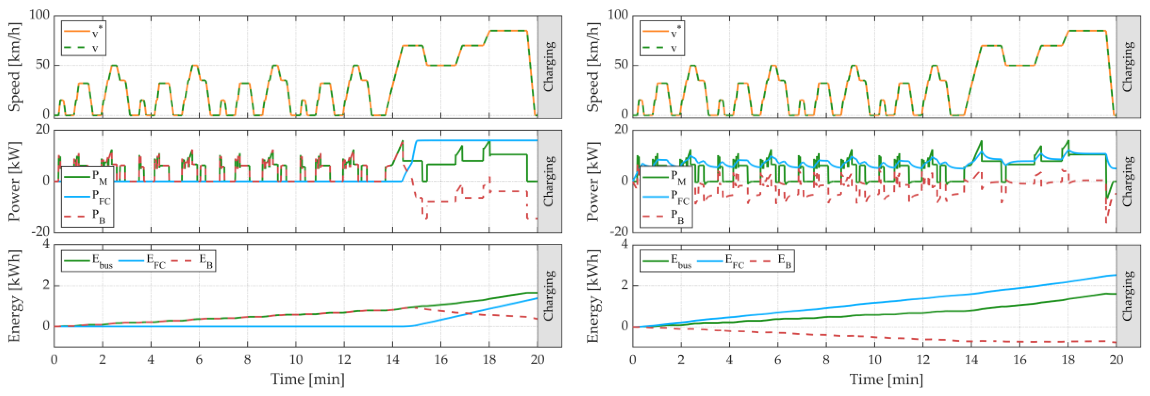
Figure 16.
Voltages, state-of-charge and costs achieved over NEDC by H-EMS (left) and S-EMS (right).
Figure 16.
Voltages, state-of-charge and costs achieved over NEDC by H-EMS (left) and S-EMS (right).

Figure 17.
Powers and energies achieved over WLTC by H-EMS (left) and S-EMS (right).
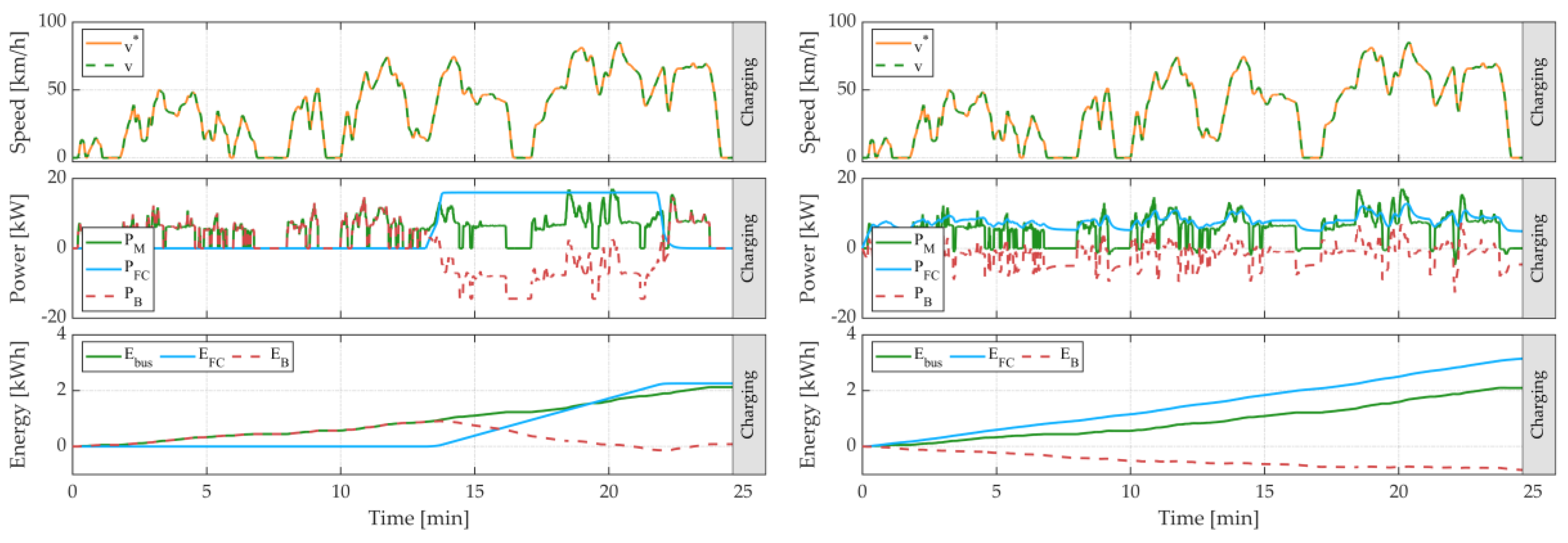
Figure 18.
Voltages, state-of-charge and costs achieved over WLTC by H-EMS (left) and S-EMS (right).
Figure 18.
Voltages, state-of-charge and costs achieved over WLTC by H-EMS (left) and S-EMS (right).

Figure 19.
Powers and energies achieved over REAL by H-EMS (left) and S-EMS (right).

Figure 20.
Voltages, state-of-charge and costs achieved over REAL by H-EMS (on the left) and S-EMS (right).
Figure 20.
Voltages, state-of-charge and costs achieved over REAL by H-EMS (on the left) and S-EMS (right).
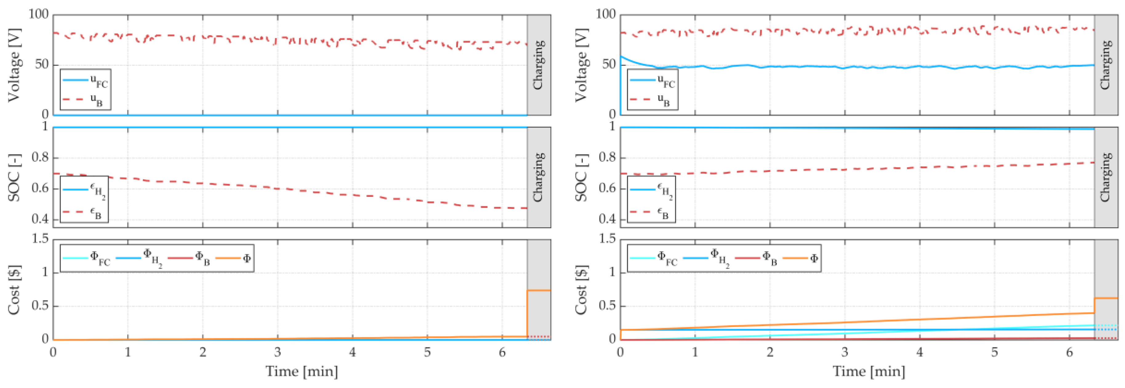
Figure 21.
Performance comparison between H-EMS (blue bars) and S-EMS (red bars) in terms of cost function contributions over different driving cycles.
Figure 21.
Performance comparison between H-EMS (blue bars) and S-EMS (red bars) in terms of cost function contributions over different driving cycles.
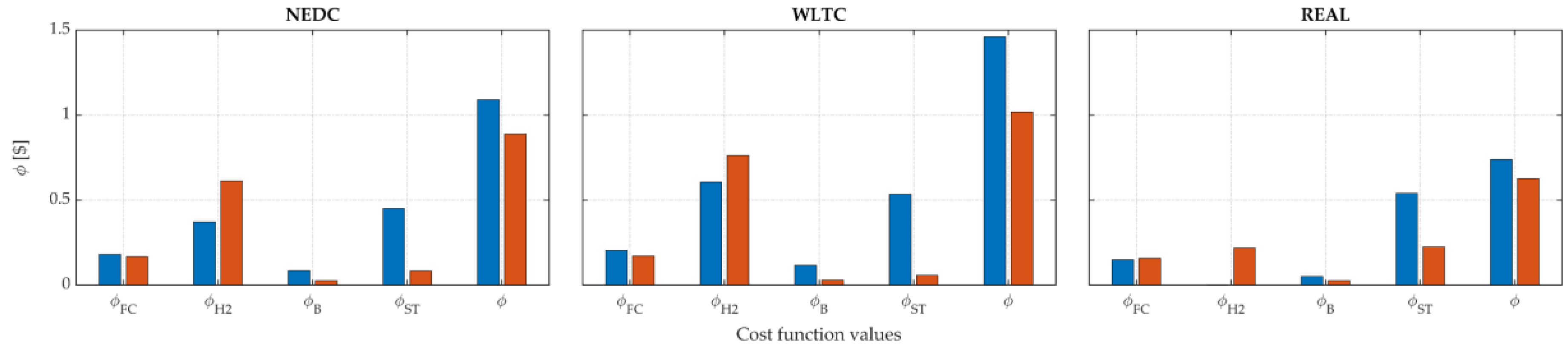
Table 1.
Cost function values (H-EMS and S-EMS).
| EMS | NEDC | WLTC | REAL | |
|---|---|---|---|---|
| ϕFC [$] | H-EMS | 0.1812 | 0.2043 | 0.1500 |
| S-EMS | 0.1665 | 0.1702 | 0.1568 | |
| ϕH2 [$] | H-EMS | 0.3720 | 0.6062 | 0.0000 |
| S-EMS | 0.6131 | 0.7625 | 0.2171 | |
| ϕB [$] | H-EMS | 0.0842 | 0.1162 | 0.0493 |
| S-EMS | 0.0259 | 0.0286 | 0.0269 | |
| ϕST [$] | H-EMS | 0.4522 | 0.5338 | 0.5405 |
| S-EMS | 0.0826 | 0.0575 | 0.2240 | |
| Φ [$] | H-EMS | 1.0897 | 1.4605 | 0.7398 |
| S-EMS | 0.8881 | 1.0187 | 0.6248 |
Table 2.
Cost function values (S-EMS and A-EMS).
| ΔT [s] | Cycle | S-EMS | A-EMS | ||||||||||
|---|---|---|---|---|---|---|---|---|---|---|---|---|---|
| - | 0 | 0 | 5 | 20 | 60 | 120 | 180 | 240 | 300 | 360 | 420 | 480 | |
| ϕFC [$] | NEDC | 0.1665 | 0.1669 | 0.1669 | 0.1669 | 0.1668 | 0.1668 | 0.1668 | 0.1669 | 0.1670 | 0.1670 | 0.1671 | 0.1672 |
| WLTC | 0.1702 | 0.1711 | 0.1711 | 0.1710 | 0.1708 | 0.1704 | 0.1704 | 0.1704 | 0.1704 | 0.1705 | 0.1705 | 0.1706 | |
| REAL | 0.1568 | 0.1571 | 0.1571 | 0.1570 | 0.1569 | 0.1567 | 0.1565 | 0.1564 | 0.1562 | 0.1561 | 0.1560 | 0.1558 | |
| ϕH2 [$] | NEDC | 0.6131 | 0.6409 | 0.6405 | 0.6391 | 0.6354 | 0.6301 | 0.6253 | 0.6207 | 0.6162 | 0.6119 | 0.6077 | 0.6037 |
| WLTC | 0.7625 | 0.7827 | 0.7825 | 0.7821 | 0.7807 | 0.7786 | 0.7749 | 0.7698 | 0.7650 | 0.7603 | 0.7558 | 0.7515 | |
| REAL | 0.2171 | 0.2246 | 0.2243 | 0.2237 | 0.2219 | 0.2192 | 0.2167 | 0.2143 | 0.2121 | 0.2099 | 0.2077 | 0.2056 | |
| ϕB [$] | NEDC | 0.0259 | 0.0290 | 0.0290 | 0.0288 | 0.0283 | 0.0276 | 0.0270 | 0.0265 | 0.0260 | 0.0255 | 0.0251 | 0.0247 |
| WLTC | 0.0286 | 0.0312 | 0.0311 | 0.0310 | 0.0308 | 0.0305 | 0.0300 | 0.0293 | 0.0288 | 0.0282 | 0.0278 | 0.0274 | |
| REAL | 0.0269 | 0.0274 | 0.0274 | 0.0274 | 0.0272 | 0.0271 | 0.0269 | 0.0268 | 0.0267 | 0.0266 | 0.0266 | 0.0266 | |
| ϕST [$] | NEDC | 0.0826 | 0.0526 | 0.0531 | 0.0545 | 0.0584 | 0.0641 | 0.0694 | 0.0744 | 0.0794 | 0.0842 | 0.0889 | 0.0935 |
| WLTC | 0.0575 | 0.0382 | 0.0383 | 0.0385 | 0.0391 | 0.0403 | 0.0441 | 0.0496 | 0.0549 | 0.0602 | 0.0652 | 0.0701 | |
| REAL | 0.2240 | 0.2149 | 0.2152 | 0.2160 | 0.2181 | 0.2212 | 0.2242 | 0.2271 | 0.0230 | 0.2326 | 0.2353 | 0.2379 | |
| Φ [$] | NEDC | 0.8881 | 0.8894 | 0.8894 | 0.8892 | 0.8889 | 0.8886 | 0.8885 | 0.8884 | 0.8885 | 0.8886 | 0.8888 | 0.8891 |
| WLTC | 1.0187 | 1.0231 | 1.0230 | 1.0226 | 1.0213 | 1.0198 | 1.0193 | 1.0191 | 1.0191 | 1.0191 | 1.0192 | 1.0195 | |
| REAL | 0.6248 | 0.6240 | 0.6240 | 0.6240 | 0.6241 | 0.6242 | 0.6244 | 0.6246 | 0.6248 | 0.6251 | 0.6255 | 0.6259 | |
© 2019 by the authors. Licensee MDPI, Basel, Switzerland. This article is an open access article distributed under the terms and conditions of the Creative Commons Attribution (CC BY) license (http://creativecommons.org/licenses/by/4.0/).
Share and Cite
MDPI and ACS Style
Serpi, A.; Porru, M. Modelling and Design of Real-Time Energy Management Systems for Fuel Cell/Battery Electric Vehicles. Energies 2019, 12, 4260. https://doi.org/10.3390/en12224260
AMA Style
Serpi A, Porru M. Modelling and Design of Real-Time Energy Management Systems for Fuel Cell/Battery Electric Vehicles. Energies. 2019; 12(22):4260. https://doi.org/10.3390/en12224260
Chicago/Turabian StyleSerpi, Alessandro, and Mario Porru. 2019. "Modelling and Design of Real-Time Energy Management Systems for Fuel Cell/Battery Electric Vehicles" Energies 12, no. 22: 4260. https://doi.org/10.3390/en12224260
Note that from the first issue of 2016, this journal uses article numbers instead of page numbers. See further details here.