Article

Fluid–Structure Interaction and Flow Redistribution in Membrane-Bounded Channels

1
Dipartimento di Ingegneria, Università degli Studi di Palermo, viale delle Scienze Ed. 6, 90128 Palermo, Italy
2
Department of Mathematical Sciences, University of Liverpool, Liverpool L3 5TR, UK
3
Associated Laboratory for Green Chemistry—Clean Technologies and Processes (LAQV), REQUIMTE, Chemistry Department, FCT, Universidade NOVA de Lisboa, 2829-516 Caparica, Portugal
*
Author to whom correspondence should be addressed.
Energies 2019, 12(22), 4259; https://doi.org/10.3390/en12224259
Submission received: 27 September 2019 / Revised: 31 October 2019 / Accepted: 5 November 2019 / Published: 8 November 2019
(This article belongs to the Special Issue Blue Energy)

Abstract

:
The hydrodynamics of electrodialysis and reverse electrodialysis is commonly studied by neglecting membrane deformation caused by transmembrane pressure (TMP). However, large frictional pressure drops and differences in fluid velocity or physical properties in adjacent channels may lead to significant TMP values. In previous works, we conducted one-way coupled structural-CFD simulations at the scale of one periodic unit of a profiled membrane/channel assembly and computed its deformation and frictional characteristics as functions of TMP. In this work, a novel fluid–structure interaction model is presented, which predicts, at the channel pair scale, the changes in flow distribution associated with membrane deformations. The continuity and Darcy equations are solved in two adjacent channels by treating them as porous media and using the previous CFD results to express their hydraulic permeability as a function of the local TMP. Results are presented for square stacks of 0.6-m sides in cross and counter flow at superficial velocities of 1 to 10 cm/s. At low velocities, the corresponding low TMP does not significantly affect the flow distribution. As the velocity increases, the larger membrane deformation causes significant fluid redistribution. In the cross flow, the departure of the local superficial velocity from a mean value of 10 cm/s ranges between −27% and +39%.

1. Introduction

1.1. Hydrodynamics in Undeformed Membrane-Bounded Systems

Electrodialysis (ED) and reverse electrodialysis (RED) are ion-exchange membrane-based technologies for producing drinking water from saline water, and for producing electric energy from the controlled mixing of two solutions of different salinity, respectively [1,2]. RED and ED units consist of a series of anion- and cation-exchange membranes alternately stacked and kept separated by means of spacers or built-in profiles, which define the channels through which the two solutions flow. A repetitive unit of a RED/ED system consists of a diluate compartment, a cation-exchange membrane, a concentrate compartment, and an anion-exchange membrane, and is commonly defined as a “cell pair”.
The hydrodynamics in the fluid-filled channels has a significant impact on several process aspects, such as the pressure drop and mass transfer. Pawlowski et al. [3] investigated the effect of the cell pair number on the pressure drop in RED stacks with a variable number of cell pairs both theoretically and experimentally. In lab-scale stacks, the pressure drop in the flow channels was found to be the dominant contribution, especially for narrower channels and lower fluid flow rates. For large-scale stacks, model simulations showed that the partial pressure drop in the branches could become dominant, leading to significant deviations from a uniform fluid flow distribution. The use of chevron-profiled membranes (instead of spacers) was observed to improve the fluid mixing in a lab-scale RED stack [4]. However, since the swelling degrees of the anion- and cation-exchange membranes used were found to be slightly different, the dimensions of the resulting corrugations were also different and in some regions of the fluid compartments, did not align perfectly well, which might cause channel deformations that affect flow patterns and mixing.
A number of authors have systematically addressed, by experimental and computational methods, the effect of the geometry of spacers or membrane profiles and of their orientation with respect to the flow. Computational fluid dynamics (CFD) has largely been employed as a powerful tool for hydrodynamic simulations and predictions. 2-D and 3-D models have been developed and, in particular, 3-D simulations have allowed considerable insight into fluid flow phenomena [5,6,7,8]. In the presence of geometrical complexities, the large computational effort and long computation time required by very fine discretization limit the applicability of CFD to the simulation of a single or a few repetitive spatially periodic domains (unit cells). Therefore, some authors, e.g., Dirkse et al. [9], Kostoglou and Karabelas [10,11], Kodým et al. [12], and Pánek et al. [13], have proposed simplified models allowing the simulation of an entire channel of different membrane systems.

1.2. Motivation and Strategy of the Present Study

To date, the hydrodynamics in membrane-bounded channels equipped with net spacers or profiled membranes has been investigated assuming an undeformed (reference or nominal) geometry. However, many membrane processes, including ED and RED, may experience membrane deformation due to a transmembrane pressure (TMP) between fluid channels [14,15,16,17,18,19,20]. For example, Hong et al. [21] performed experimental and numerical studies of an RED stack with 200 cell pairs, showing a high pressure difference between seawater and fresh water channels.
The transmembrane pressure between concentrate and diluate compartments is an important module design parameter. In particular:
  • In the ideal case of a uniform (along the whole channel) transmembrane pressure (TMP), a relatively simple chain of effects and consequences would be triggered: (a) Membrane/channel deformation; (b) changes in the friction coefficients in both fluid compartments with respect to those in the undeformed configuration; and, finally, (c) consequent changes in the solutions flow rates for any given inlet-to-outlet imposed pressure drop. Such TMP effects in ED and RED processes were documented in our previous studies [22,23], which revealed a significant influence of membrane deformation on the hydrodynamics and mass transfer in channels equipped with different profiled membranes.
  • In the realistic case of a non-uniform TMP, the above chain becomes a closed loop (a two-way fluid–structure interaction, FSI) made up of: (a) Space-dependent membrane/channel deformation; (b) space-dependent changes in the friction coefficients, f, in both fluid compartments; (c) consequent space-dependent changes in the flow rates for any given inlet-to-outlet imposed pressure drop; (d) space-dependent changes in the frictional pressure losses and, thus, in the pressure distribution in both channels; and, finally, (e) changes in the spatial distribution of TMP (leading us back to point a). Once an equilibrium configuration is attained by the system, the flow distribution will generally turn out to be uneven (redistribution), also affecting the concentrations, solute mass transfer rates, and electric current densities.
To the best of the authors’ knowledge, the present work is the first attempt to investigate the above phenomena at the cell pair scale (of course, assuming a stack to be made up of identical cell pairs, the same description applies also at the stack scale). In principle, a two-way FSI model could be implemented in a sufficiently powerful simulation tool, such as COMSOL Multiphysics® or Ansys®. However, 3-D simulations of an entire channel equipped with spacers or profiled membranes would require an inordinate computational effort. Therefore, a hybrid 3-D/2-D modelling approach was chosen, following a strategy similar to that proposed by Kostoglou and Karabelas for undeformed channels in pressure-driven membrane processes [10,11].
The coupling between 3-D and 2-D simulations can be summarized as follows:
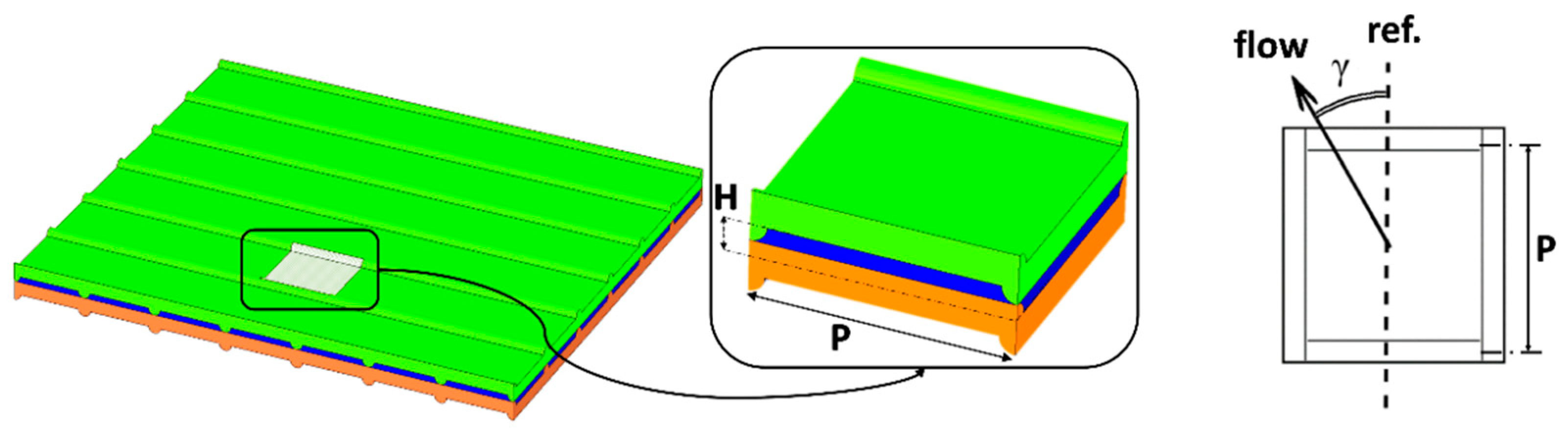
  • At the small scale of the unit cell (periodic domain identified by the membrane profiles), fully three-dimensional structural mechanics simulations were conducted by using the Ansys-Mechanical® code in order to compute the deformation of membranes/channels under different values of the transmembrane pressure, TMP, as discussed in a previous paper [22].
  • Still at the unit cell scale, fully three-dimensional CFD simulations were conducted for each deformed configuration using the Ansys-CFX® code; these simulations provided the relation between the flow rate and driving pressure gradient (hydraulic characteristic) as a function of the amount of deformation, and thus of the applied TMP, as discussed in the same paper [22].
  • In the present study, focused on the larger cell pair scale, the above results were summarized in the form of a correlation between the apparent hydraulic permeability (itself a function of the flow rate) and the transmembrane pressure, as will be discussed in Section 2.2.
  • Finally, the above information was fed to a 2-D simplified model of the cell pair as will be described in Section 2.4 and Section 2.5.
In particular, at the cell pair scale, a two-dimensional, porous medium approach for FSI simulation was developed in the present paper. Each fluid compartment was simulated as a 2-D domain characterized by a continuous distribution of pressure, flow rate, deformation, and permeability, and the continuity equation along with a generalized Darcy equation for a continuous porous medium were solved by an in-house code, involving an iterative algorithm, to evaluate the fluid distribution in both channels of a cell pair.

2. Materials and Methods

2.1. From a Small- to Large-Scale Description of Membrane-Bounded Channels

In our previous works [22,23], in order to investigate the flow characteristics in fluid-filled channels provided with profiled membranes (either in their nominal, i.e., undeformed configuration, or deformed by a transmembrane pressure), the “unit cell” approach was employed. In particular, Figure 1 shows how a periodic unit can be isolated from a fluid channel delimited by profiled membranes of the overlapped crossed filaments (OCFs) type. The central inset shows a detail of the shape of the profiles; they can be modelled as semi-cylinders protruding from both membrane sides at 90° with respect to each other. The geometry investigated in the present work is characterized by P/H = 8.
The following definitions are used throughout this study. First, the channel thickness, H, is defined under undeformed conditions as the distance between the plane regions of opposite membranes. The equivalent channel thickness, h, is defined as the ratio of the fluid volume in a unit cell to the projected membrane area (P2 for a square-planform unit cell). Note that in an undeformed channel, h is <H due to the volume occupied by the membrane profiles; in a compressed channel, h is always <H; in an expanded channel, h may be either <H or even >H. Values of h under different load conditions are reported in Table A1 of Appendix A.
The superficial velocity, U s , along a generic direction, s, is defined as the ratio between the flow rate through a cross section of the channel orthogonal to s, having width W, and its undeformed and void area H × W. The interstitial velocity, Uinter,s, along the same generic direction, s, is defined as the volume average of the s-component of the actual fluid velocity in the unit cell, and can be computed as UsH/h. It takes into account both the presence of membrane profiles and the possible deformation (compression or expansion) of the channel.
Following the approach adopted in previous papers [5,6,22,23], the velocity and length scale used for the definition of the Reynolds number were the superficial velocity, Us, and the hydraulic diameter of the void and undeformed plane channel, 2H:
R e = 2 U s H ν .
This choice allows a better appreciation of the effects of the membrane profiles and of the membrane/channel deformation. The superficial velocity was also used in the definition of drag-related quantities, such as the friction coefficient and the hydraulic permeability (see below).
The friction characteristics of a channel bounded by OCF-profiled membranes, previously computed by fully 3-D CFD simulations [22], were expressed in terms of a mean Darcy friction coefficient, fs:
f s = | p s | 4   H ρ U s 2 ,
where | p s | is the driving pressure gradient along the direction, s; ρ is the fluid density; and Us and H were defined previously.
The dependency of fs on the flow attack angle was systematically investigated both for profiled membrane configurations and for spacer-filled channels. The former results (see, for example, Figure 7 in [22]) showed that for OCF profiles with P/H = 8, up to Re ≈ 100, the equivalent friction coefficient varied in a negligible way with the flow attack angle, γ, thus exhibiting an isotropic behavior, and that no pressure gradient orthogonal to the main flow direction arose.
The equivalent friction coefficient, fs, was proportional to Re−1 (i.e., the relation between the velocity and pressure drop was linear) only up to Re ≈ 10, indicating a regime of creeping flow characterized by the self-similarity of the flow field. At higher Re, the dependence of the pressure drop on the velocity became nonlinear due to inertial effects.
In the whole range of Re ≤ 100 investigated, the flow was assumed to be steady. This assumption is justified by our previous experimental and direct numerical simulation studies for the closely related geometry of spacer-filled channels [24], in which unsteadiness was observed only for Re > 300 even at the much lower pitch to height ratio of P/H = 2. Even larger values of the transitional Reynolds number can be expected at the present large P/H (8).
At the larger scale of a whole cell pair (and thus of a whole stack), like that investigated in the present study, the single unit cell is no more resolved, and the flow can be described as flow in a porous medium [10,11,25]. Under the assumption of flat channels, the generic channel can be treated as a two-dimensional domain. In view of the above-discussed invariance of the equivalent friction coefficient with the flow attack angle, the permeability can be assumed to be isotropic and the relation between the pressure gradient and the superficial velocity is a generalized Darcy equation:
p s = μ K a p p U s ,
where μ is the fluid viscosity and Kapp is a (scalar) apparent permeability, independent of the flow direction, s. At low Reynolds numbers (i.e., <10), Kapp attains a constant value, K, independent of the velocity, Us, and Equation (3) takes the form of the classical Darcy law. At higher Reynolds numbers, when inertial effects occur, the Darcy law is replaced by the Darcy–Forchheimer equation:
p s = μ K U s + ρ F U s 2 ,
containing two characteristics of the porous medium, namely a Darcy permeability, K, and a Forchheimer coefficient, F [26]. Equation (4) can still be expressed in the form of Equation (3) provided the apparent permeability is expressed as Kapp = K/(1 + ρKFUs/μ).
The apparent permeability is related to the friction factor, fs, by:
K a p p = 4 μ H ρ U s 1 f s .
The value of Kapp deduced from the friction coefficient using Equation (5) can then be employed in Equation (3) to estimate the superficial velocity associated with a given pressure gradient in the fluid domain. A straightforward solution of Equation (3) is not possible if the channel permeability varies in space as a function of the local transmembrane pressure and the closed-loop interactions mentioned in Section 1.2 occur. The following sections present a mathematical model based on an iterative algorithm dealing with this issue, thus computing the steady-state fluid distribution in the channels in the presence of significant membrane deformation.

2.2. Computational Domain and Modelling Assumptions

The model simulates two whole adjacent channels, a diluate (DIL, low electrolyte concentration) and a concentrate (CON, high electrolyte concentration), together with the associated AEM and CEM membranes (the “cell pair”). Figure 2 shows a schematic representation of a cell pair equipped with OCFs-profiled membranes and a sketch of the computational “molecules” adopted in the present model for the formulation of balance equations in the discrete form.
Membranes are not actually included in the computational domain. The hydrodynamic effects of the profiled membranes and their deformation are taken into account by using constitutive equations expressing the channel’s apparent permeability as a function of the transmembrane pressure and superficial velocity, as defined in Section 2.1.
As discussed above, such equations can be derived from our previous 3-D mechanical-fluid dynamics investigation at the lower scale level of a unit cell [22,23]. The sign convention for TMP adopted in the present paper is consistent with that adopted in our previous work: TMP is positive if the concentrate channel is compressed and the diluate channel is expanded, whereas it is negative if the concentrate channel is expanded and the diluate channel is compressed.
For the geometry investigated here (OCF profiles with a pitch-to-height ratio of P/H = 8), the apparent permeability, Kapp, of the concentrate channel is reported in Figure 3 as a function of the superficial velocity, Us, for different TMP values. It can be observed that the assumption of Darcyan flow (i.e., of a linear dependence of the velocity on the pressure gradient, with K constant and independent of Us) is well satisfied only for velocities of the order of a few cm/s (Re ≈ 10 for H = 200 μm), which are common in RED but rather low in ED.
The other assumptions made in the present model are:
(a)
The flow field is steady.
(b)
The fluid properties are constant and are the same in both the DIL and CON channels (the values ρ = 997 kg/m3 and μ = 8.89·10−4 Pa·s were used in the examples discussed in this paper).
(c)
AEM and CEM membranes share the same mechanical properties and profiles geometry, so that the same correlation for the channel apparent permeability applies to both channels.
(d)
Transmembrane water transport (due to osmotic flow and electro-osmotic drag) is neglected. Therefore, the inlet flow rate coincides with the outlet flow rate. This assumption is justified by the fact that the transmembrane water flow rate is much less than the main water flow rate along the channels. For example, even in the unrealistically extreme case of ED with a large concentration gradient (seawater–freshwater), a high current density (100 A/m2), large channel length/thickness ratio (3000, e.g., L = 0.6 m, H = 200 μm), low superficial velocity (1 cm/s) in both channels, large membrane osmotic permeability (10 mL/(m2 h bar)), and hydration number of 7 (water molecules/ion), the total transmembrane water flow rate estimated by elementary balances is less than 8% of the axial flow rate of each solution.
In addition, the following conventions are adopted:
  • Flow rates exiting a computational block are assumed to be positive, while flow rates entering a block are assumed to be negative.
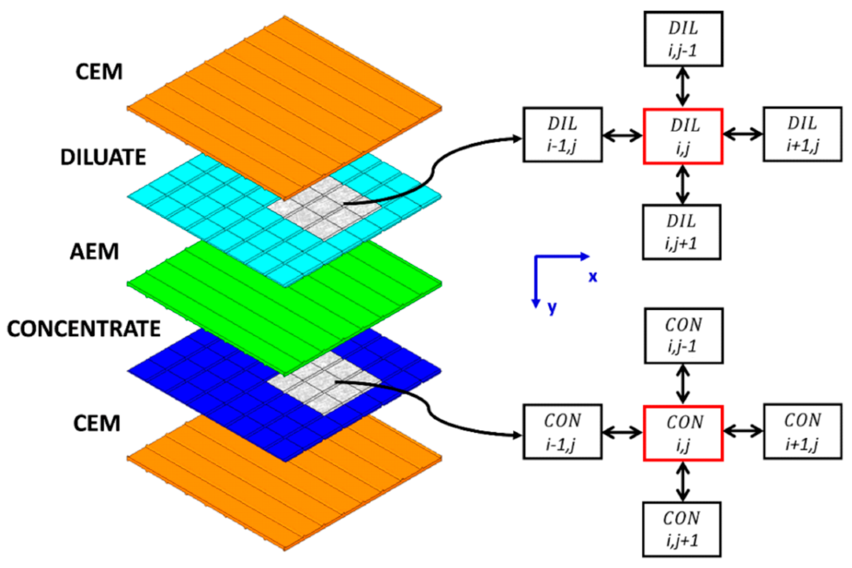
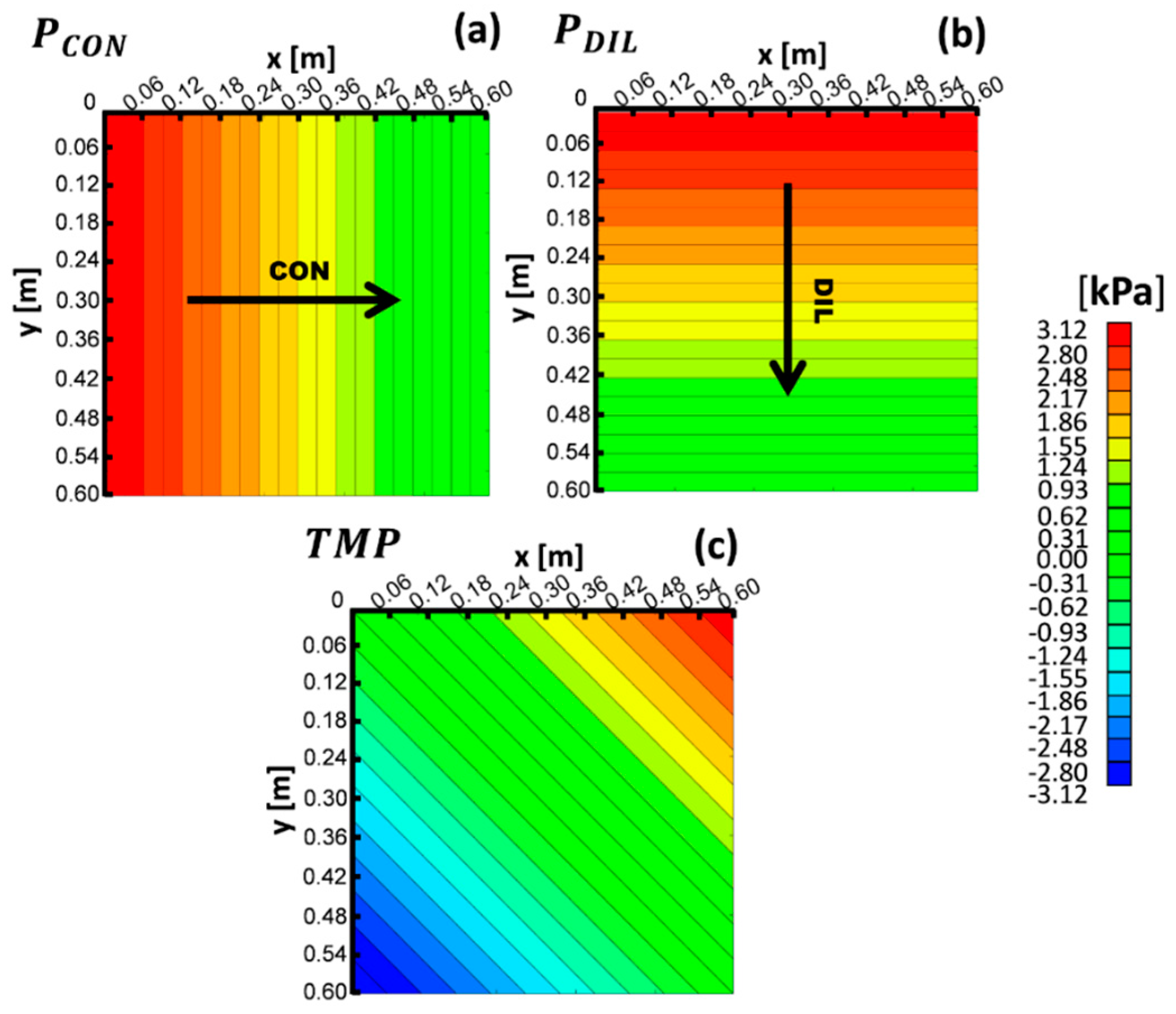
  • The TMP is calculated as the difference between the local pressures in the DIL and CON compartments ( T M P i , j = P i , j D I L P i , j C O N C ), so that, as mentioned above, it is positive when DIL is expanded and CON compressed. By definition, if the CON compartment locally experiences a given value of TMP, at the corresponding location, the DIL compartment is subjected to −TMP.
The model was implemented in the Matlab® environment.

2.3. Discretized Continuity Equation

We assume that each of the two coupled CON and DIL channels, of an overall size of Lx × Ly, is divided into Nx × Ny rectangular blocks of size Δx = Lx/Nx, Δy = Ly/Ny. Each channel is treated as a continuous, porous, two-dimensional medium, and the block size, being an arbitrary computational construct, is unrelated to the size of the individual unit cell as defined by the membrane profiles.
For either channel, considering a steady state flow regime and making reference to the sketch in Figure 2, the continuity equation at the generic computational block, i, j, can be written as:
U i , j + 1 i , j + U i + 1 , j i , j U i , j i 1 , j U i , j i , j 1 = 0 ,
in which each U is the volume flow rate through the corresponding block interface divided by HΔx or HΔy (undeformed and void-channel area of the same interface). Superscripts indicate the grid block from which the flow exits while subscripts indicate the block into which the flow is entering. Signs are attributed according to convention I.

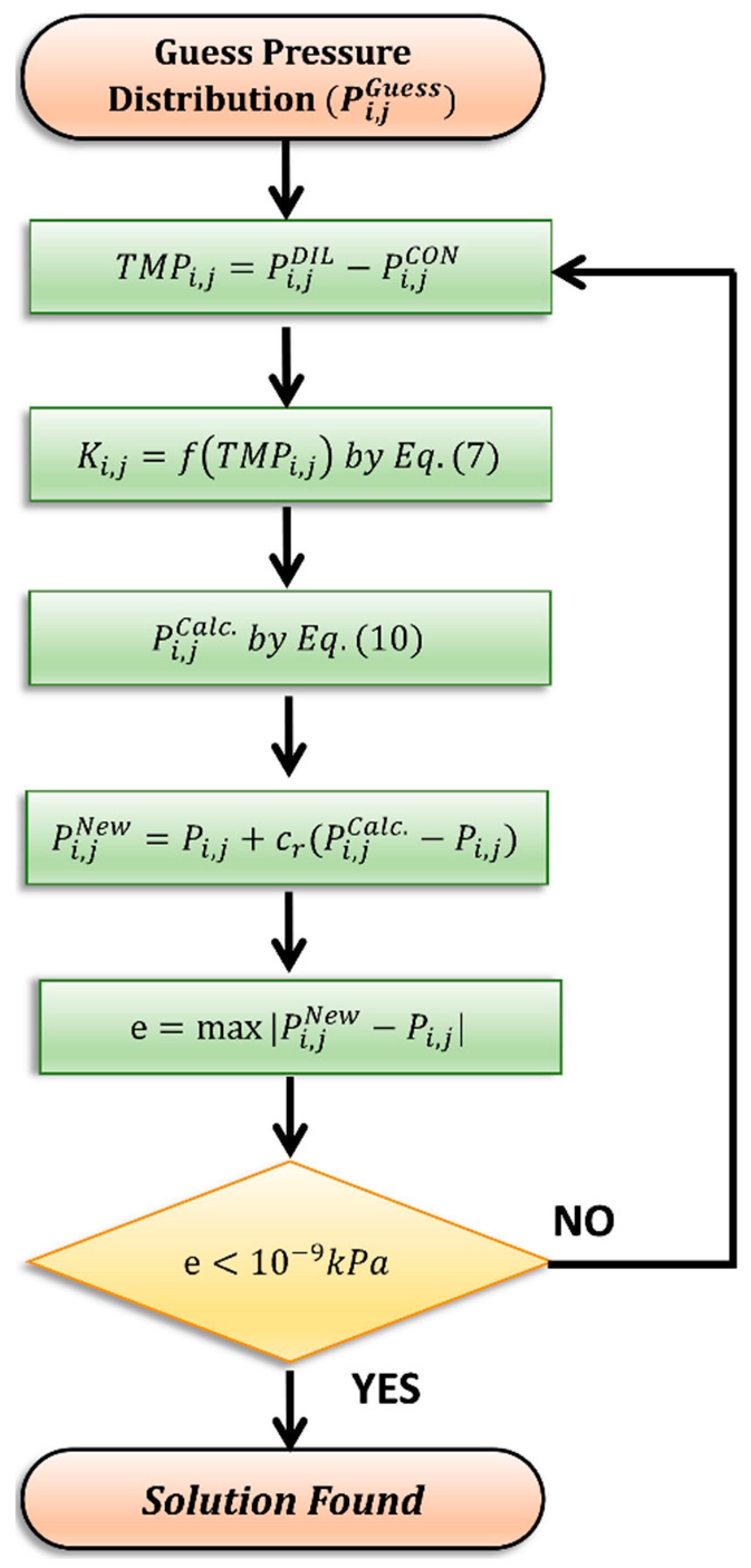
2.4. Discretized Darcy Equation for the Case of Low Velocity

In the limit of low Us, the apparent permeability in Figure 3 becomes a function of transmembrane pressure only and is shown in Figure 4.
The function K(TMP) can be approximated well by a quadratic function:
K = 2.405 · 10 13 · TMP 2 3.4 · 10 11 · TMP + 1.656 · 10 9 ,
in which K is in m2 and TMP is in kPa.
The non-Darcyan range of higher velocities, in which Kapp depends not only on TMP but also on Us, requires a slightly more complex treatment and will be separately discussed in Section 2.5.
By approximating the derivatives in the Darcy equation (Equation (2)) with reference to the block sizes Δx or Δy, the superficial velocities of the fluid can be expressed as:
U i + 1 , j i , j = K i , j μ · P i + 1 , j P i , j Δ x ,
U i , j + 1 i , j = K i , j μ · P i , j + 1 P i , j Δ y ,
and are similar for the velocities at interfaces (i − 1, j) and (i, j − 1).
By substituting Equations (8) and (9) into Equation (6), and considering for simplicity Δx = Δy, the pressure in block (i, j) can be expressed as:
P i , j C a l c = K i , j · P i + 1 , j + K i , j · P i , j + 1 + K i 1 , j · P i 1 , j + K i , j 1 · P i , j 1 K i 1 , j + 2 K i , j + K i , j 1 .
The steady state pressure distribution in deformed channels must simultaneously satisfy Equation (10) (which was derived from the continuity and Darcy equations) and the constitutive law, e.g., Equation (7), expressing the dependence of the channel’s permeability on the local TMP. An iterative algorithm was developed in order to perform this coupling; its flow chart is schematically shown in Figure 5 and is briefly commented below.
First, a guess for pressure is imposed in both channels at each grid block ( P i , j G u e s s ). Random values distributed between −40 and +40 kPa were used in the present applications. Then, the local TMP is calculated by using convention II, and the K i , j values in both channels are determined by using Equation (7). A new pressure value, P i , j C a l c . , is computed at each block (i, j) by using Equation (10). Finally, under-relaxation is applied before starting a new iteration:
P i , j N e w = P i , j + c r ( P i , j C a l c . P i , j ) ,
where c r is an under-relaxation factor for which a value of 0.7 was chosen as a reasonable trade-off between the computing time and convergence stability. The algorithm terminates when the maximum difference between the old and new pressures over all grid blocks becomes less than a prescribed small value (10−9 kPa). Once convergence is attained, superficial velocities are computed from Equations (8) and (9).

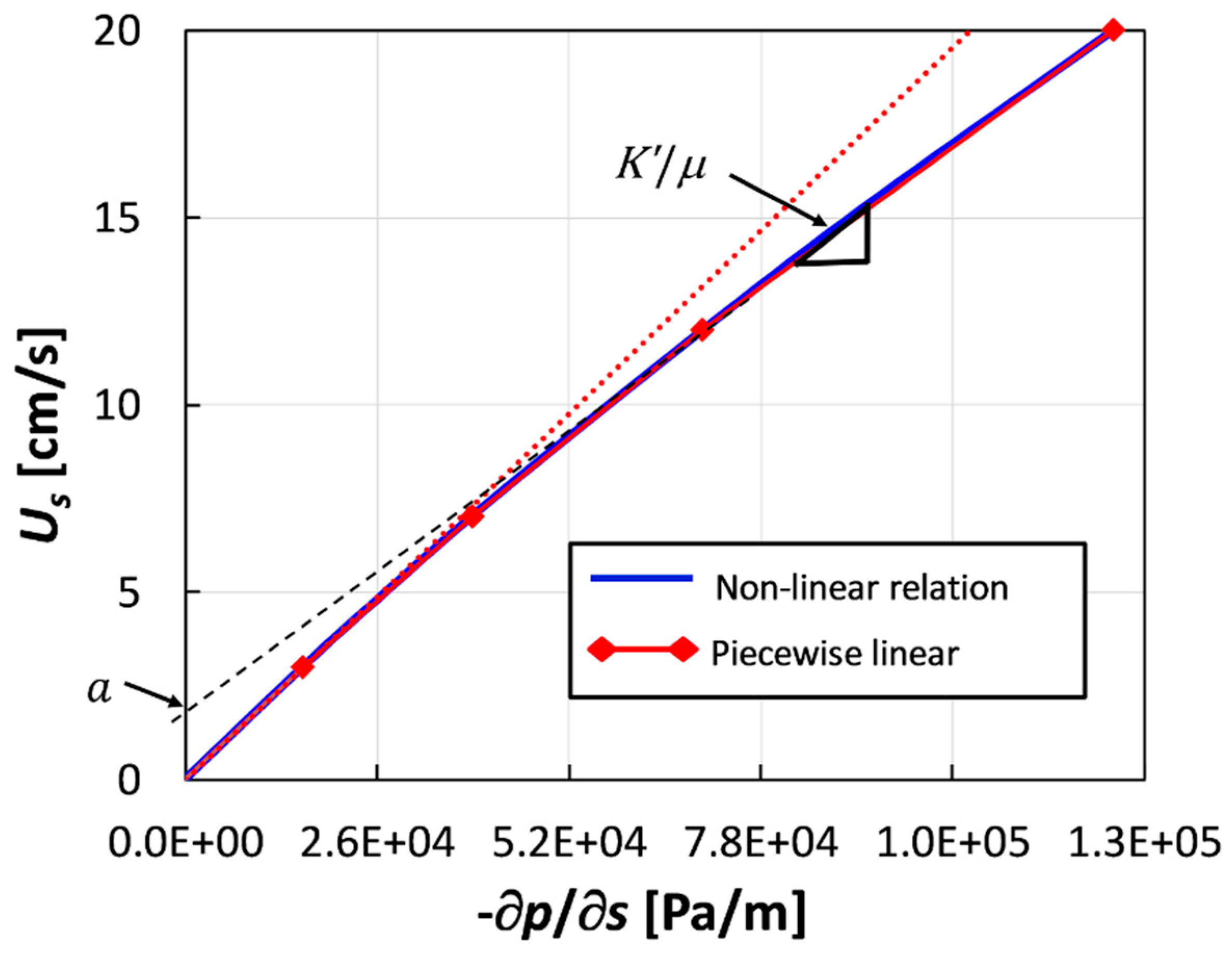
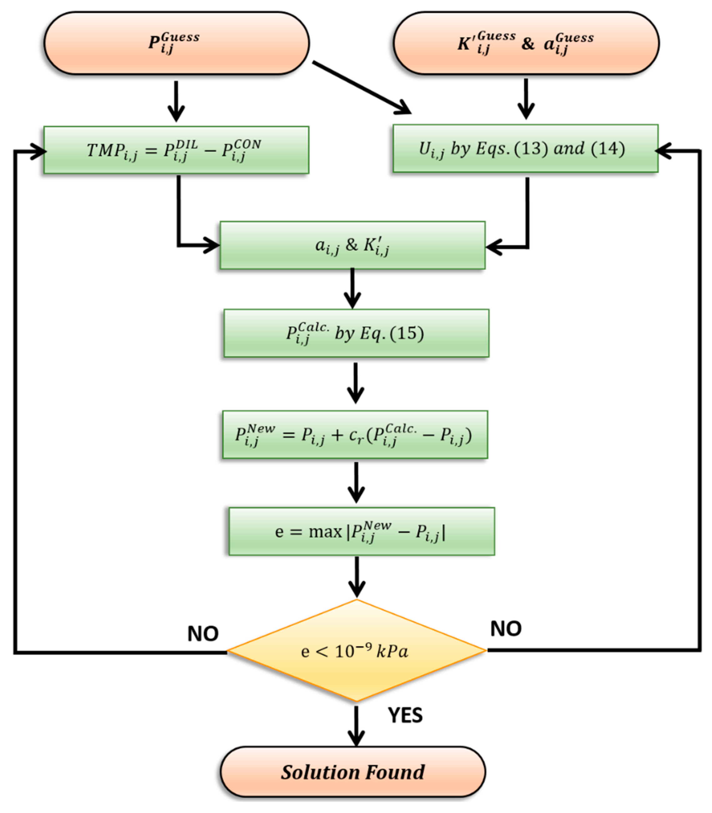
2.5. Model Adjustment for Non-Darcyan Flow Regime

Industrial electro-membrane processes, especially ED, often experience fluid velocities larger than a few cm/s and channel thicknesses larger than 200 μm [1,27]. Under these conditions, yielding Reynolds numbers of the order of 102, the linear relation between the velocity and pressure gradient expressed by the Darcy law is no longer valid, i.e., Kapp depends on Us. For the sake of clarity, the relation between the velocity and pressure gradient obtained from 3-D CFD simulations [22] is reported in Figure 6 for the undeformed case; in the presence of deformation, a similar graph applies for each value of TMP. The blue solid line represents the Us vs. ∂p/∂s relation computed by CFD while the dotted red line represents the linear extrapolation of the behavior observed in the limit of low velocity. A significant departure from the linear behavior is observed for velocities larger than ~10 cm/s. Therefore, in order to investigate higher flow regimes without excessively modifying the proposed model, a piecewise linear fitting (represented in Figure 6 by the red line segments separated by symbols) was applied to capture the dependence of the apparent channel permeability on the velocity. Each linear segment is identified by its slope, K’/μ, and its intercept, a, as shown in Figure 6, with K’ = K and a = 0 in the first segment.
The same procedure was repeated for all the values of TMP investigated between −40 and +40 kPa; Table A2 and Table A3 in Appendix A report the slopes and intercepts of each straight line segment.
Accordingly, the Darcy equation (Equation (2)) can be replaced by:
U s = K μ ( p s ) + a ,
in which K′ and a are constant for each segment of the piecewise linear approximation.
In the discretized form, Equations (8) and (9) are modified as follows:
U i + 1 , j i , j = K i , j , x μ · P i + 1 , j P i , j Δ x s g n ( P i + 1 , j P i , j ) · a i , j x ,
U i , j + 1 i , j = K i , j , y μ · P i , j + 1 P i , j Δ y s g n ( P i , j + 1 P i , j ) · a i , j y ,
and are similar for velocities (i − 1, j) and (i, j − 1). The terms a i , j x , a i , j y and K i , j , x / μ , K i , j , y / μ are the intercepts and the slopes of the straight line segments, respectively. The terms a i , j x   and   a i , j y are multiplied by the sign of the pressure difference between two consecutive computational blocks to account for the direction of the flow. The terms K i , j , x and K i , j , y may be different despite the isotropy of the medium because of the different values of the velocity along x and y. At low velocity, both K i , j , x and K i , j , y reduce to K i , j , which is the proportionality constant of the Darcy equation (Equation (2)) while the term a i , j vanishes.
Substituting Equations (13) and (14) into Equation (6), and considering for simplicity Δx = Δy, one obtains:
P i , j C a l c = 1 K i , j , y + K i , j , x + K i 1 , j , x + K i , j 1 , y { ( K i , j , x · P i + 1 , j + K i , j , y · P i , j + 1 + K i 1 , j , x · P i 1 , j + K i , j 1 , y · P i , j 1 ) + μ Δ x [ a i , j y s g n ( P i , j + 1 P i , j ) + a i , j x s g n ( P i + 1 , j P i , j ) a i 1 , j x s g n ( P i , j P i 1 , j ) a i , j 1 y s g n ( P i , j P i , j 1 ) ] } .
Equation (15) must be employed instead of Equation (10) to evaluate the pressure value at each computational block in either channel. It requires an initial distribution of K i , j , x , y and a i , j x , y to calculate the flow velocity at each computational block. Therefore, some additional steps must be added to the algorithm, as illustrated by the flowchart in Figure 7.
First, initial (guess) values, P i , j G u e s s ,   K i , j , G u e s s , and a i , j G u e s s , of pressures and non-Darcyan parameters are set in both channels at each grid block and the corresponding TMP and velocities are calculated by using convention II and Equations (13) and (14), respectively. On the basis of the local TMP and superficial velocities, new K i , j , x , y and a i , j x , y values are computed by linear interpolation of the data reported in Table A2 and Table A3. Then, pressures P i , j C a l c are calculated by using Equation (15). Finally, after applying under-relaxation using Equation (11) (as in the Darcyan case), the error is evaluated and, until it decreases below the prescribed value, a new iteration is performed.
Guess values, K i , j , G u e s s and a i , j G u e s s , too far from the equilibrium values may hinder the convergence of the algorithm. Therefore, in the present work, the guess pressure distribution, P i , j G u e s s , was obtained by running the simplified (Darcyan) model while the guess a i , j x , y values were set to zero at each block and the guess K i , j , x , y values were assumed equal to the K i , j values of the simplified model.

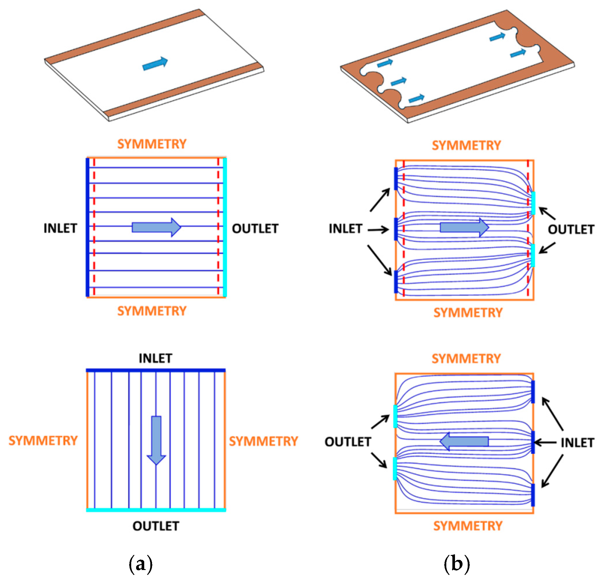
2.6. Flow Arrangement and Boundary Conditions

The most common fluid flow arrangements employed in RED and ED applications are: (i) parallel flow, (ii) counter flow, and (iii) cross flow. The advantages and disadvantages of these layouts have amply been discussed in the literature [1,2]. Parallel flow assures the lowest TMP values between fluid channels, thus minimizing leakages and membrane deformation issues (ideally TMP = 0 if the two solutions share the same velocity and physical properties and the channels share the same geometrical configuration). On the other hand, the parallel flow arrangement suffers from a strong axial variation of concentration difference, which, in turn, reduces the driving force in RED and increases the energy consumption in ED. Counter flow is characterized by a more uniform distribution of the concentration difference along the channel length but exhibits the largest TMP. Finally, the cross flow layout has shown a more uniform electric current distribution and promising process performances in RED [28].
In the present work, the fluid flow distribution in a square stack with a 0.6-m side was analyzed in the cross flow and counter flow arrangements. For the aforementioned reasons, parallel flow does not pose significant TMP issues and therefore was not investigated. A channel length of 0.6 m allowed for an investigation of the superficial velocities up to ~10 cm/s with an inlet-outlet pressure drop below 40 kPa, corresponding to the highest TMP value for which correlations for K were obtained. This size is close to that of square prototype stacks that have actually been used in RED applications [28,29]. The choice of a square stack simplifies the calculations and the interpretation of the results obtained. Of course, the model could also be applied to rectangular geometries, which are often employed in industrial ED units [30].
The two flow arrangements investigated in the present work are shown in Figure 8. In cross flow, fluid enters and exits each channel through two opposite slots of height H in the lateral gasket located beside the channel area where membrane profiles are, running through the whole width, W, of each channel. In the case of counter flow, inlets and outlets are shorter slots connecting the channels with manifolds orthogonal to the membranes; they were simulated here as straight segments, three at the inlet and two at the outlet. The inlet slots were placed 3 cm away from the upper and lower side walls and the outflow ones were 14 cm away. All slots were 10 cm wide and the distance between adjacent slots was 12 cm.
In all cases, the pressure was set to zero at the outlet boundaries and to a uniform value, Pin, at the inlet boundaries. In the cross flow case, values of 3.12, 16.29, and 34.3 kPa were set for Pin, yielding superficial velocities in the undeformed channels of 1, 5, and 10 cm/s, respectively. Only the value of Pin = 34.3 kPa was investigated in the case of the counter flow configuration, where it yielded a superficial velocity in the undeformed channels of ~8.5 cm/s.
In regard to the side boundaries, where neither inlet nor outlet boundaries were specified, the most physically appropriate boundary condition would be the no slip one. However, since no slip conditions are not fully consistent with the Darcy approximation, pressure symmetry conditions were used instead. CFD simulations for the counter flow configuration were performed in which either symmetry or no slip wall conditions were imposed on the side boundaries, and discrepancies of less than 1% were observed in the computed pressure distribution.
Grid dependence, i.e., the effect of the number of channel blocks on the model’s results, was analyzed by comparing five grids of increasing resolution. Results for a single undeformed channel were also compared with the CFD predictions obtained using the Ansys-CFX® code. Details of these comparisons are reported in Appendix B.

3. Results and Discussion

3.1. Cross Flow Arrangement

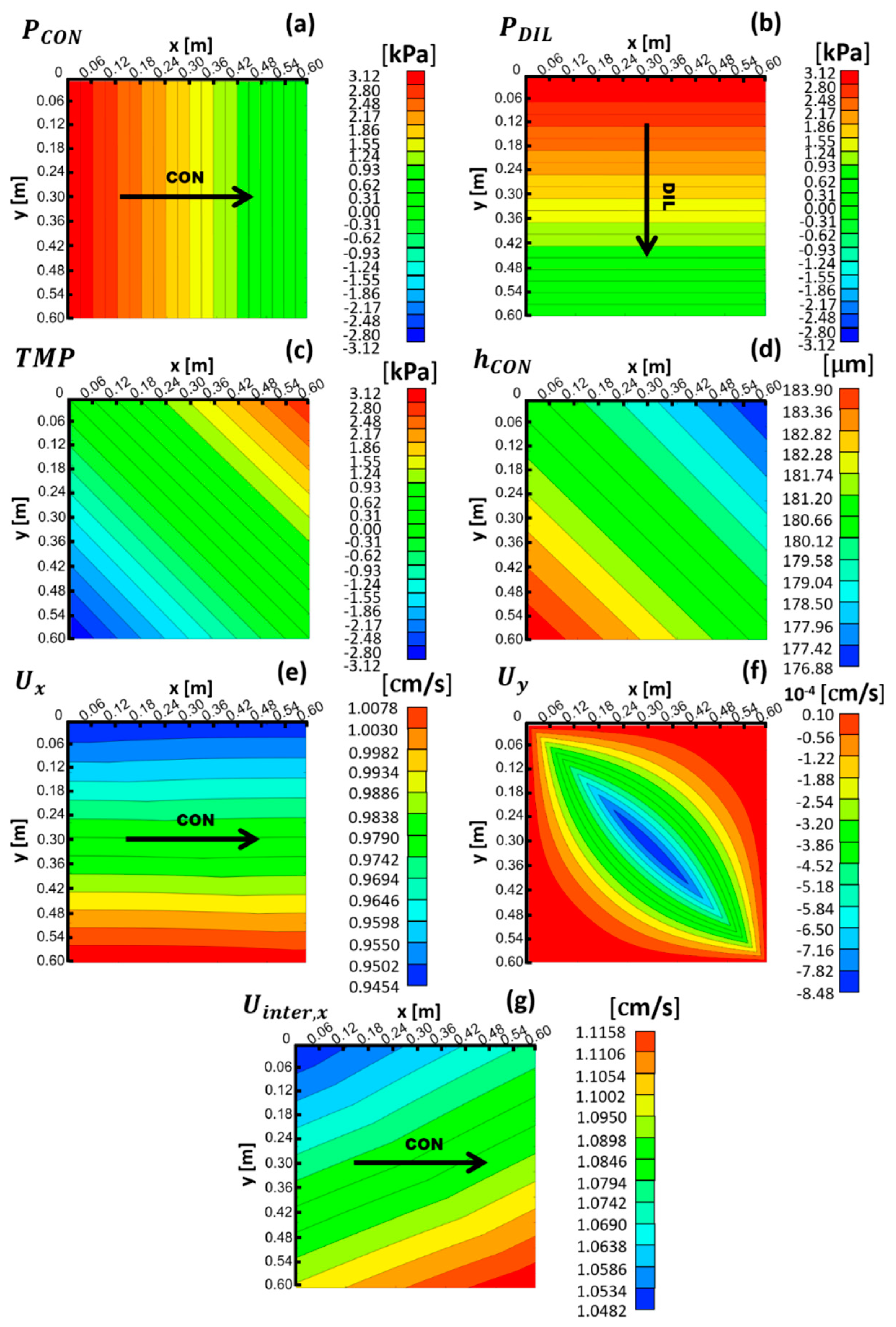
3.1.1. Low Velocity Case (Pin − Pout = 3.12 kPa, Yielding Us ≈ 1 cm/s)

Pressure maps and TMP for the cross flow configuration with an inlet pressure of 3.12 kPa (yielding Us = 1 cm/s, being s either x for the CON channel or y for the DIL channel) are shown in Figure 9 for the case in which membrane deformation effects are not taken into account. In each channel, pressure decreases linearly along the flow direction. The resulting TMP exhibits an anti-symmetric behavior about the descending diagonal of the channel, attaining its lowest value at the bottom left corner and the highest value at the top right corner. Velocity maps are not shown since a flat distribution exists.
Results obtained for the same cross flow stack of Figure 9, but taking membrane deformation into account, are shown in Figure 10. Note that at the low velocity considered here, the behavior of the channel regarded as a porous medium is purely Darcyan (see Figure 6). The effects of membrane deformation are too small to be seen in the pressure maps (a,b), and also the TMP is almost the same as in the undeformed case (Figure 9c).
Figure 10d reports the equivalent height, h, of the concentrate channel, which exhibits an anti-symmetric trend about the channel’s descending diagonal (as TMP) but attains its lowest value at the top right corner and its highest value at the bottom left corner (opposite to TMP), and changes by only about ±2% with respect to the undeformed channel equivalent height (180 μm). This modest membrane deformation only slightly affects the distribution of the streamwise superficial velocity component (Ux), which is shown in map (e) for the concentrate channel. This quantity exhibits a stratification in the direction orthogonal to the main flow direction, with a mean value 〈Us〉 of ~0.976 cm/s (almost the same as in the undeformed case) and a variation of about ±3%.
For the sake of completeness, the superficial velocity component along the direction orthogonal to the main flow ( U y ) is also reported in map (f). U y is ~4 orders of magnitude lower than the streamwise component, Ux, and exhibits a symmetric distribution about the channel’s descending diagonal.
Finally, map (g) reports the interstitial velocity. This quantity presents relative variations of about ±3% to 4%, similar to those observed for the superficial velocity, but a different distribution, which results from the combined variations of the superficial velocity, Us, and channel equivalent height, h.

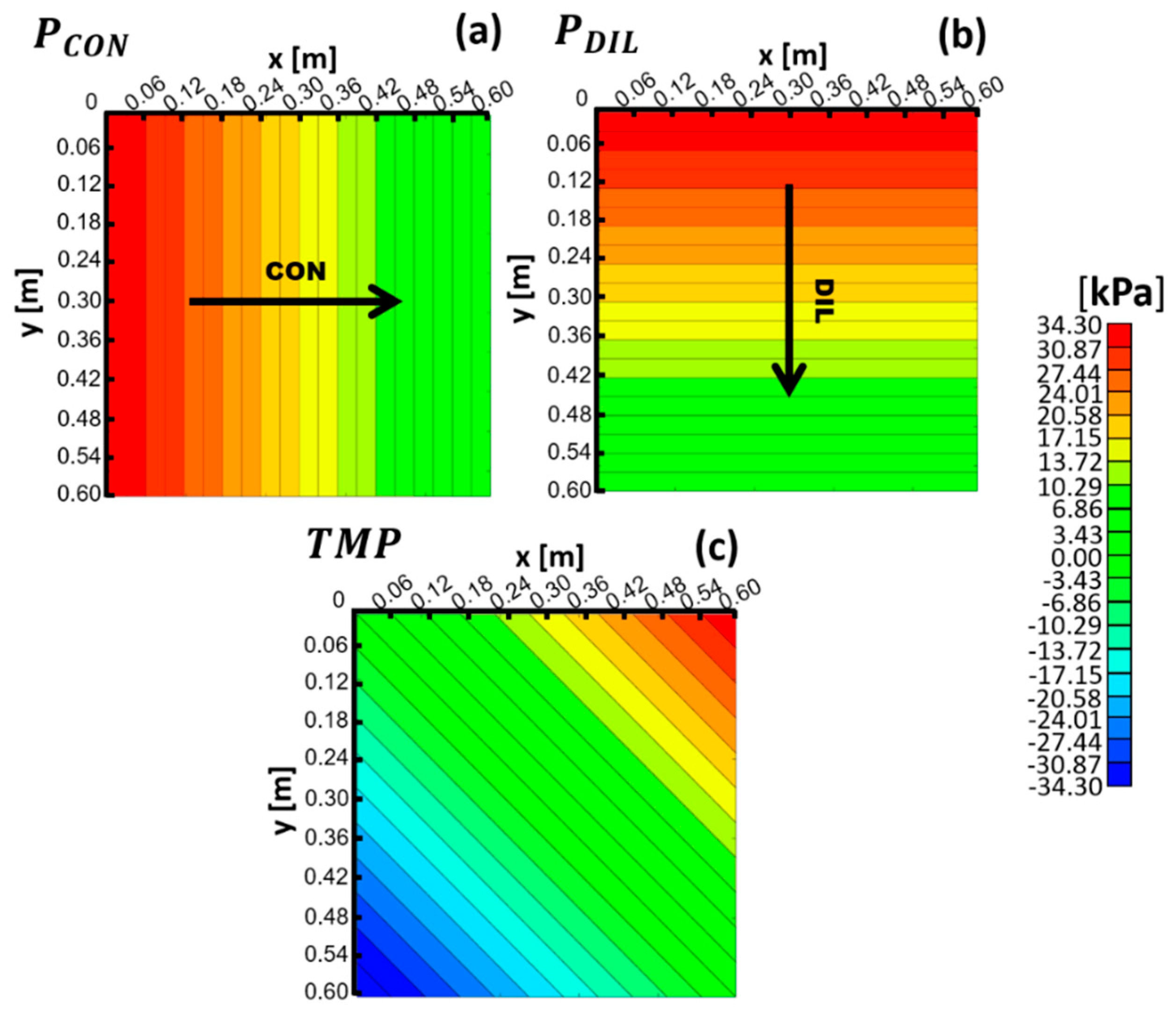
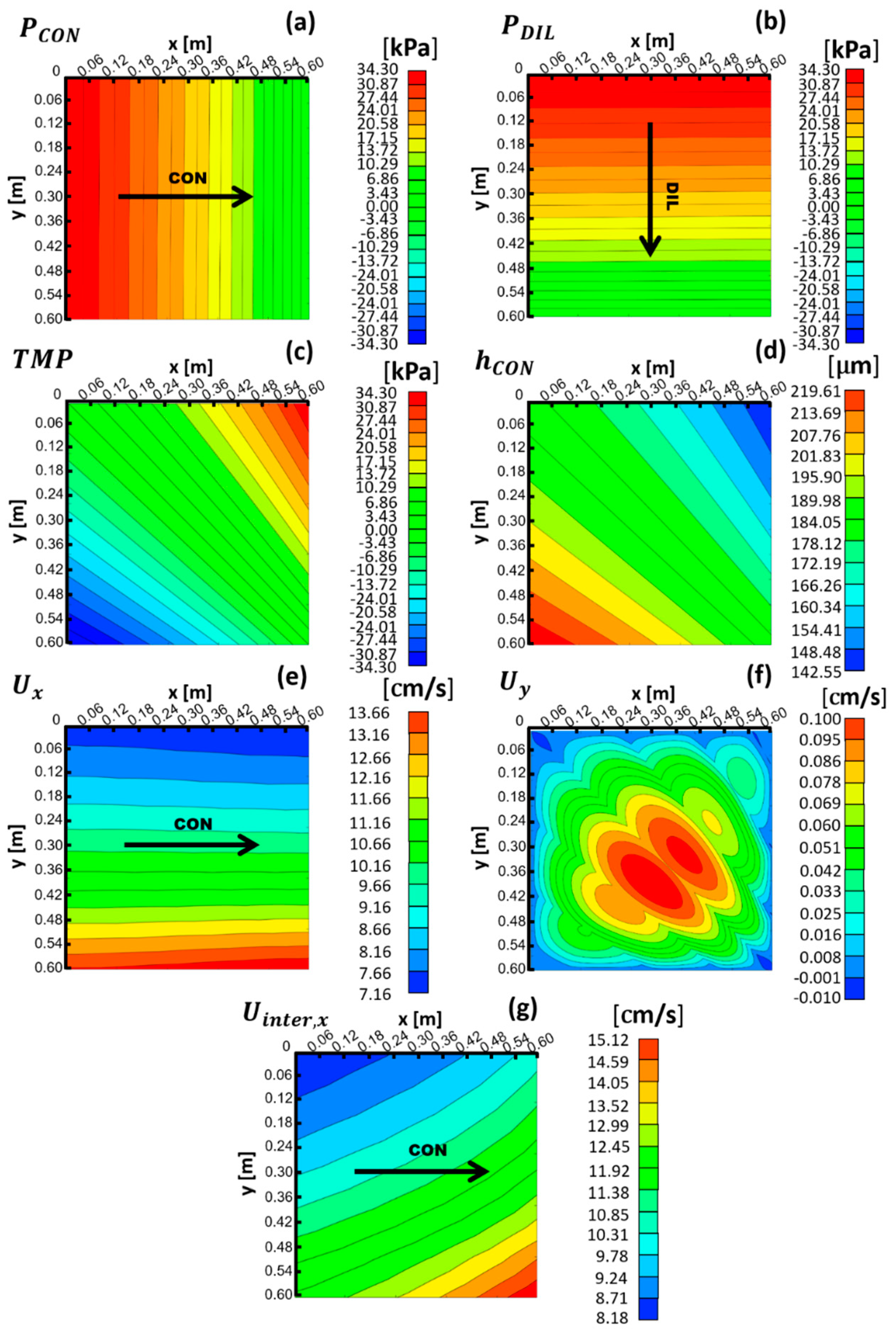
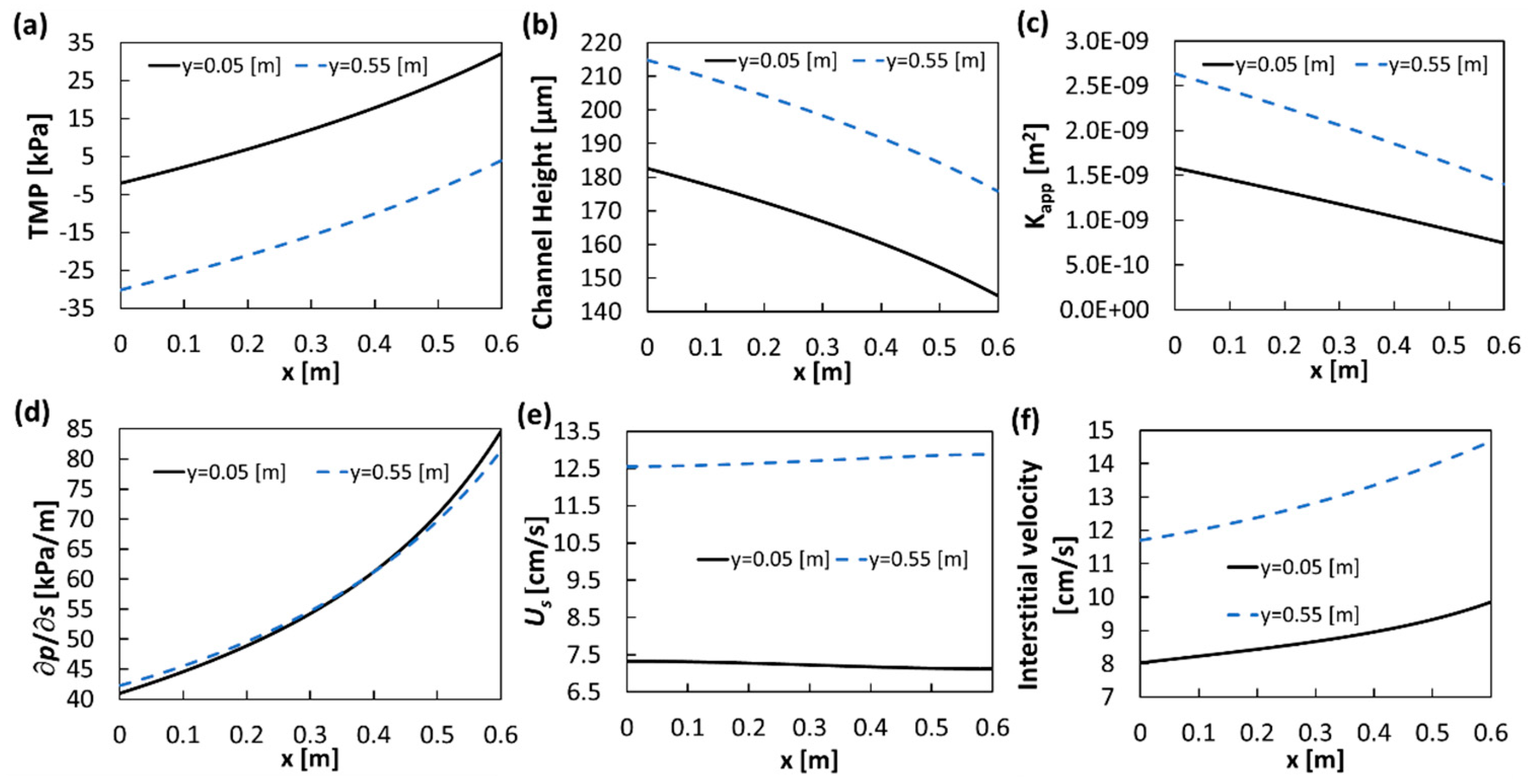
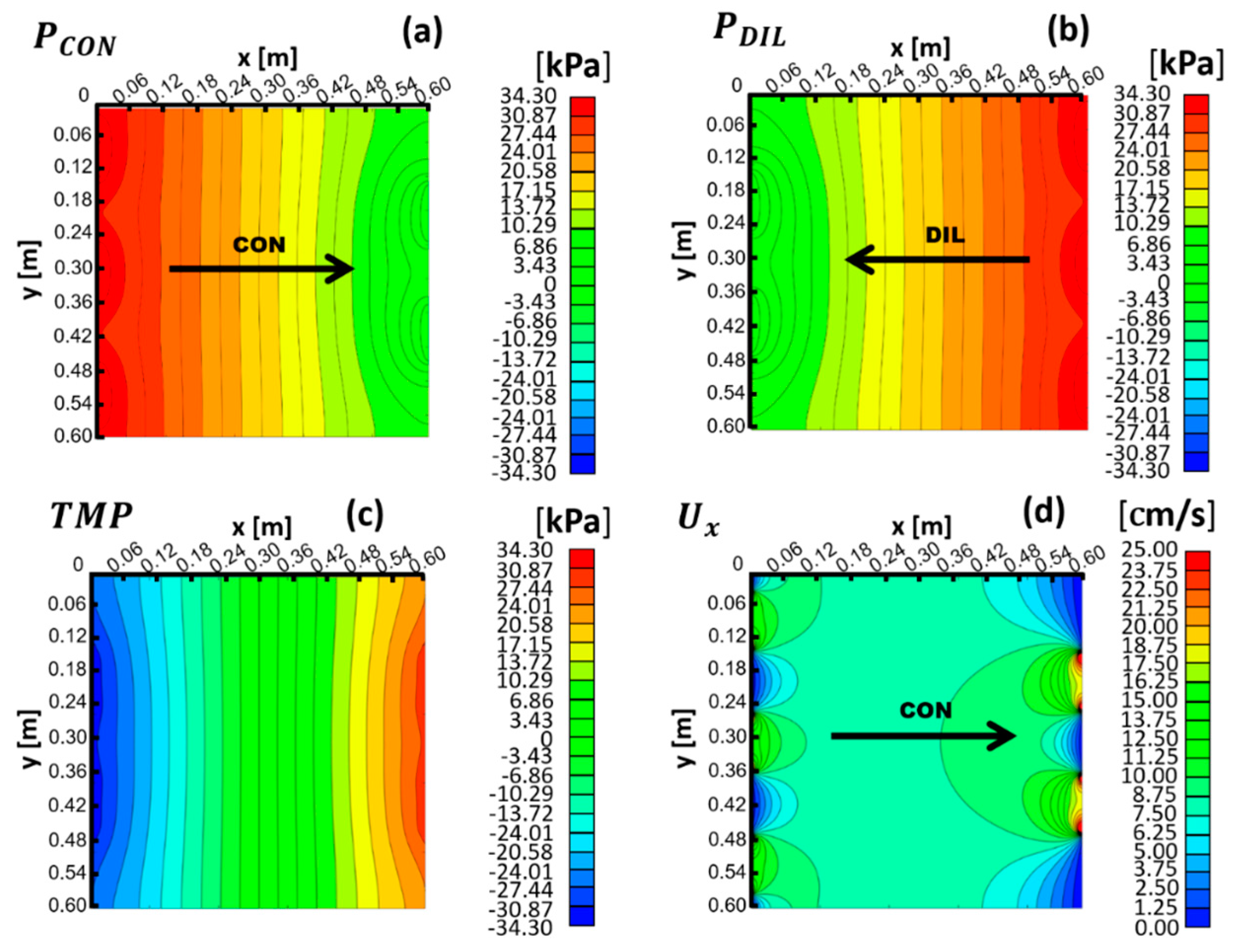
3.1.2. Higher Velocity Case (Pin − Pout = 34.3 kPa, Yielding Us ≈ 10 cm/s)

The same cross flow configuration considered in the previous section, see Figure 9 and Figure 10, was also investigated for an inlet pressure of 34.3 kPa, yielding Us ≈ 10 cm/s along the main flow direction.
The results for the case in which membrane deformation effects are not taken into account are shown in Figure 11. In the absence of membrane deformation, the pressure in the channels decreases linearly along the flow directions as in the lower velocity case, and TMP shows the same anti-symmetric behavior about the descending diagonal of the channel.
Results for the case in which membrane deformation effects are taken into account are reported in Figure 12. In this case, the behavior of the channel regarded as a porous medium is significantly non-Darcyan, as can be observed in Figure 6.
Membrane deformation significantly affects the pressure distribution in the channels, as can be seen in maps (a,b). Specifically, the pressure distribution is not linear, but the pressure gradient increases as the fluid approaches the outlet regions. The TMP, map (c), is still anti-symmetric about the descending diagonal, but now the iso-TMP lines are no longer parallel to this diagonal but converge towards the bottom right corner.
Map (d) reports the concentrate channel’s equivalent height, h, which varies by about ±20% with respect to that of the undeformed channel (180 μm). As shown in map (e), the higher membrane deformation (compared to the low velocity case) enhances the stratification along y of the superficial velocity, Us, with a mean value 〈Us〉 of 9.82 cm/s (1.8% reduction with respect to the undeformed case) and a maximum variation of +39% in the lower region of the stack (close to y = 0.6 m) and −27% in the upper region (close to y = 0).
Map (f) reports the secondary superficial velocity component along the direction orthogonal to the main flow direction (Uy, in the concentrate channel). This quantity is now two to three orders of magnitude lower than the streamwise component, Us, and exhibits a more complex distribution than in the lower velocity case of Figure 10f.
Finally, map (g) reports the interstitial velocity. It shows a similar trend as for the Us = 1 cm/s case but presents much larger relative variations (about ±35%) and a much more non-uniform gradient.
For the same test case (cross flow at Us ≈ 10 cm/s in the presence of membrane deformation), a better understanding of the behavior of the different quantities in Figure 12 can be achieved by considering the profiles of different variables along the main flow direction (x for the concentrate channel). Figure 13 reports such profiles as obtained at two spanwise locations, namely, y = 0.05 m (upper region of the maps in Figure 12) and y = 0.55 m (lower region of the same maps).
The transmembrane pressure TMP (graph a) increases along the x direction at both y locations, and varies from about 0 to about 28 kPa along the line y = 0.05 m and from about −34 to 0 kPa along the line y = 0.55 m. As a consequence, the concentrate channel equivalent height, graph (b), decreases from ~180 to ~145 μm, i.e., from undeformed to compressed, at y = 0.05 m, and from ~215 to ~180 μm, i.e., from expanded to undeformed, at y = 0.55 m. Thus, the channel is compressed in the upper region of the stack and expanded in the lower one.
As shown in graph (c), the channel’s apparent permeability decreases along the x direction following the trend of the channel’s equivalent height, in accordance with Figure 3. The streamwise pressure gradient, graph (d), increases along the flow direction x (by about the same amount at both y locations) to compensate for the decreasing permeability while the mass flow rate remains constant. The superficial velocity, Us, graph (e), can be calculated as the product of the pressure gradient by the channel’s apparent permeability. As a result, Us is lower at y = 0.05 m than at y = 0.55 m, since the pressure gradient is almost the same at the two locations, while the permeability is lower in the upper-compressed region of the channel than in the lower-expanded one.
Graph (f) shows profiles of the interstitial velocity, defined in Section 2.1 as UsH/h. This quantity increases along the flow direction x at both y locations because the superficial velocity, graph (e), varies much less than the channel equivalent height, graph (b). Moreover, the interstitial velocity is lower at y = 0.05 m (upper, compressed region of the channel) than at y = 0.55 m (lower, expanded region) because the superficial velocity varies along y more than the equivalent channel height.

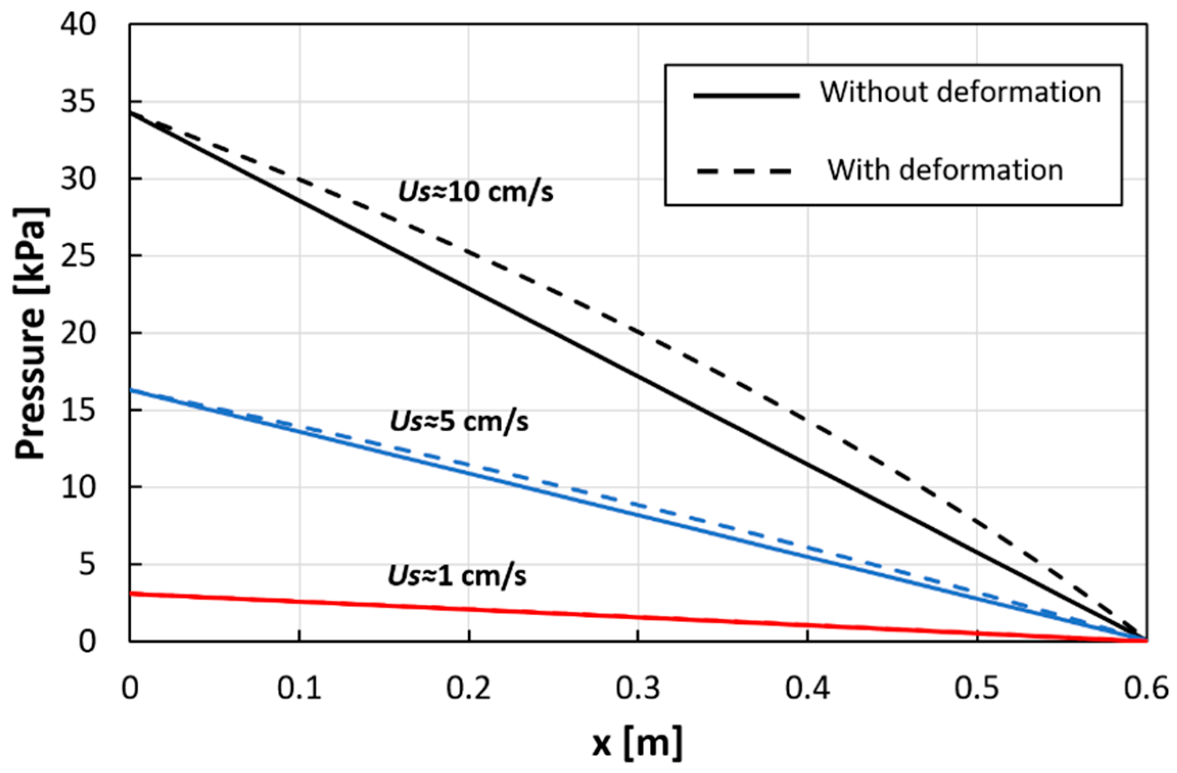
3.1.3. Pressure Profiles for All Cross Flow Cases

Pressure profiles along the x direction near the lower edge of the concentrate channel (y = 0.55 m) are shown in Figure 14 for imposed pressure drop values (PinPout) of 3.12, 16.29, and 34.3 kPa, respectively, yielding 〈Us〉 values of approximately 1, 5, and 10 cm/s. Both the undeformed and the deformed conditions are considered.
Note that the same pressure drops are imposed in undeformed and deformed conditions. The reduction of the mean fluid velocity 〈Us〉 under deformed conditions is small (1.8% for PinPout = 34.3 kPa, as mentioned in Section 3.1.2, and practically negligible for lower pressure drops).
In the absence of deformation, pressure decreases linearly with x. At 〈Us〉 ≈ 1 cm/s, membrane deformation is small, as already discussed in Section 3.1.1, and does not significantly affect the pressure profile. As the velocity, and thus the TMP, increases, pressure profiles depart from the linear trend. Cubic polynomial functions are found to fit the pressure profiles well when membrane deformation becomes considerable.

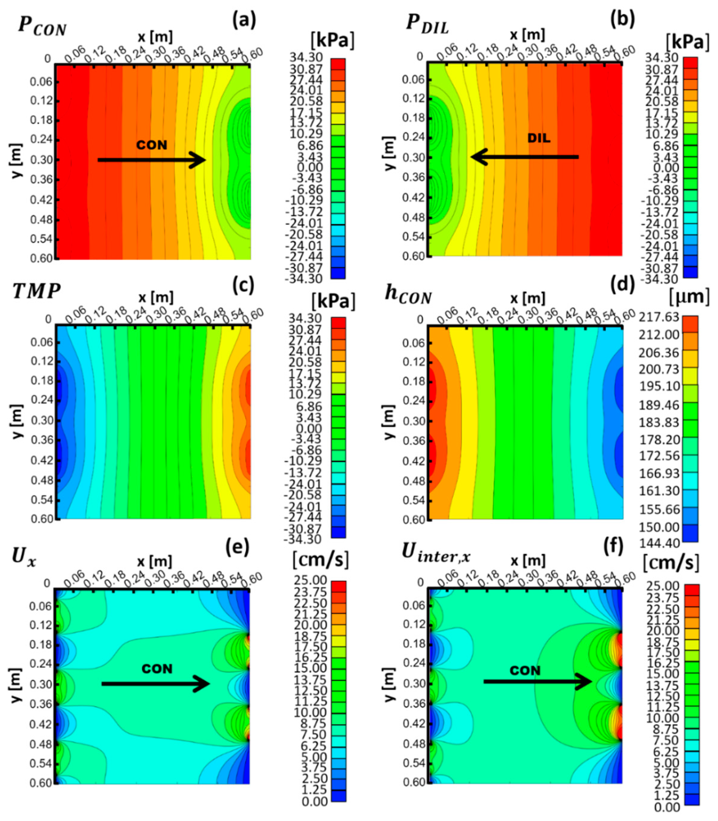
3.2. Counter Flow Arrangement

In the counter flow arrangement, only one pressure inlet value (34.3 kPa) was investigated. This pressure value is the same used for the cross flow case discussed in Section 3.1.2, where it yielded U s ≈ 10 cm/s. In the present case, due to the different geometry of the inlet and outlet regions (see Figure 8), the resulting superficial velocity in the absence of membrane deformation is Us ≈ 8.5 cm/s (with s corresponding to x). Note that pressure changes due to abrupt area variations, present in this configuration, are not taken into account by the model, but this is not a severe limitation because, at the present low velocity, these terms (proportional to the kinetic pressure. ρ U s 2 /2) are negligible compared to the distributed losses (order of 0.01 kPa, compared to the imposed inlet–outlet pressure variation of 34.3 kPa). This conclusion is also supported by the comparison with the CFD results in Appendix B.2.
For the case of no membrane deformation, maps of the pressure in both channels, TMP, and superficial velocity along the main flow direction in the concentrate channel are shown in Figure 15. In each channel, the inlet and outlet regions can be observed in which the geometry of the openings significantly affects the pressure distribution, see maps (a,b); outside these regions, p is mainly stratified with a uniform gradient along the flow direction x. Of course, the two distributions are identical apart from a reflection about the vertical midline. As a result, TMP in map (c) is anti-symmetric with respect to the vertical midline and ranges from negative to positive values spanning an interval twice that exhibited by the pressure in each of the separate channels. The streamwise superficial velocity in the concentrate channel, map (d), exhibits complex details in the inlet and outlet regions and is almost flat in the central region.
Figure 16 reports results obtained in the presence of membrane deformation. Pressure distributions (see maps (a,b)) show that the pressure gradient along x increases towards the outlet regions, where the channel is compressed. In each channel, a larger pressure non-uniformity is observed near the (two) outlet openings than near the (three) inlet ones. The non-uniform pressure gradient trends partially compensate when the pressure difference, i.e., TMP, is computed, yielding a more uniform gradient, map (c). Note that the shape of the TMP iso-lines reflects the geometry of the outlets more than that of the inlets.
The channel equivalent height in the concentrate compartment exhibits the opposite trend to TMP, decreasing from its highest value of ~218 μm in the inlet region to its lowest value of ~144 μm in the outlet region. The superficial velocity distribution, map (e), is qualitatively similar to that obtained in the undeformed case (Figure 15d), but its mean value 〈Us〉 is now ~7.5 cm/s, ~12% lower than that computed in the undeformed case (~8.5 cm/s). This result can be attributed to the asymmetric behavior of the hydraulic permeability, which varies less under compression than under expansion.
Finally, map (f) shows the interstitial velocity in the concentrate channel. This quantity changes slightly with respect to the superficial velocity without significant fluid redistribution phenomena.

4. Conclusions

A novel fluid–structure interaction model was developed to investigate the flow distribution in ED/RED stacks in the presence of membrane deformations arising from the pressure difference between adjacent channels (transmembrane pressure, TMP). An iterative algorithm was developed to solve the continuity and Darcy equations in two neighboring channels, treated as porous media, taking into account the spatial variation of their hydraulic permeability as a function of the local TMP. The model was extended to also deal with non-Darcyan flow conditions, thus allowing its use for fluid velocities higher than a few cm/s, typical of electrodialysis channels. The computational accuracy of the present model was proven for the case of undeformed channels by comparing its results with those obtained by performing CFD simulations.
Square stacks with 0.6-m sides equipped with profiled membranes of the overlapped crossed filament type (pitch 1.6 mm, nominal channel height 200 μm, Young modulus 150 MPa, membrane thickness 120 μm) were investigated both in the counter and cross flow operation mode at superficial fluid velocities ranging from 1 to 10 cm/s.
In the case of the cross flow configuration, at low velocities (e.g., 1 cm/s), the membrane deformation was small and did not significantly alter the results with respect to the undeformed configuration. On the other hand, at the higher velocity of 10 cm/s, the channel equivalent height was found to vary by up to about ±20% with respect to its mean value; the superficial velocity also exhibited considerable non-uniformity, with departures from the mean value ranging from −27% to +39%. The effect of the membrane deformation also altered the pressure variation in each channel along the corresponding main flow direction, so that the pressure profile became non-linear and exhibited a cubic trend. For an imposed pressure drop of 34.3 kPa, the superficial velocity decreases from 10 cm/s in the undeformed case to a mean value of 9.82 cm/s (1.8% reduction) in the simulation taking into account deformation effects.
In the case of counter flow, the model showed its ability to deal with partial inlet and outlet openings, representative of the manifold configuration typical of this operation mode. Also, in this case, the maximum variation of the channel equivalent height with respect to its mean value was ±20%, but there were no significant flow redistribution phenomena. However, as an effect of the asymmetric behavior of the hydraulic permeability under compression and expansion, deformation caused a reduction of flow rate of 12% for an imposed pressure drop of 34.3 kPa.
A grid dependence study was conducted and showed that for the case of cross flow, 2-D grids with just 60 × 60 blocks were sufficient to yield satisfactory results. For the case of counter flow, the presence of small details in the geometry of the inlets and outlets made finer grids, e.g., 120 × 120 blocks, necessary.
On the whole, the present study demonstrates that membrane deformation and its effects can be significant in large stacks with cross flow or counter flow arrangements. Note that membrane deformations and flow redistribution effects may become even larger, e.g., if thinner membranes or a larger pitch to height ratio were employed. Therefore, process modelling and optimization tools should take these aspects into consideration. The model developed in the present study was successfully applied to a specific geometrical configuration and specific membrane mechanical properties but could easily be extended to different geometries and operating conditions.

Author Contributions

Conceptualization, A.C. and M.C.; methodology, G.B., L.G. and M.C.; software, G.B.; validation, G.B., L.G. and M.C.; formal analysis, G.B., L.G. and M.C.; investigation, G.B.; resources, A.C., A.P. and G.M.; data curation, G.B., L.G. and M.C.; writing—original draft preparation, G.B.; writing—review and editing, G.B., L.G., A.C., S.V. and M.C.; visualization, G.B. and M.C.; supervision, A.C., A.P., S.V., M.C. and G.M.; project administration, A.C., M.C. and G.M.; funding acquisition, A.C., A.P. and G.M.

Funding

This research was carried out within the REvivED water project (Low energy solutions for drinking water production by a REvival of ElectroDialysis systems). This project has received funding from the European Union’s Horizon 2020 research and innovation programme under Grant Agreement no. 685579 (www.revivedwater.eu).

Conflicts of Interest

The authors declare no conflict of interest.

Appendix A. Dependence of Equivalent Channel Height and Channel Hydraulic Permeability on TMP

Appendix A.1. Equivalent Channel Height

As discussed in Section 2.1, the equivalent channel height is defined here as the ratio between the fluid volume and projected area. Table A1 reports fluid volumes and corresponding equivalent channel heights for the unit cell of channels delimited by OCF-profiled membranes characterized by H = 200 μm and P = 1600 μm (P/H = 8, projected area P2 = 2.56 mm2) for TMP varying between −40 and +40 kPa.
Channel height values were fit by a second-order polynomial, which was implemented in the Matlab® program (h is in μm, TMP in kPa):
h = 6.0025 · 10 4 · T M P 2 1.1285 · 10 7 · T M P + 180 .
Table A1. Channel fluid volume and equivalent height as a function of TMP.
TMP [kPa]V [mm3]h [μm]
400.349136
300.376147
200.404158
100.432169
00.462180
−100.491192
−200.521203
−300.550215
−400.579226

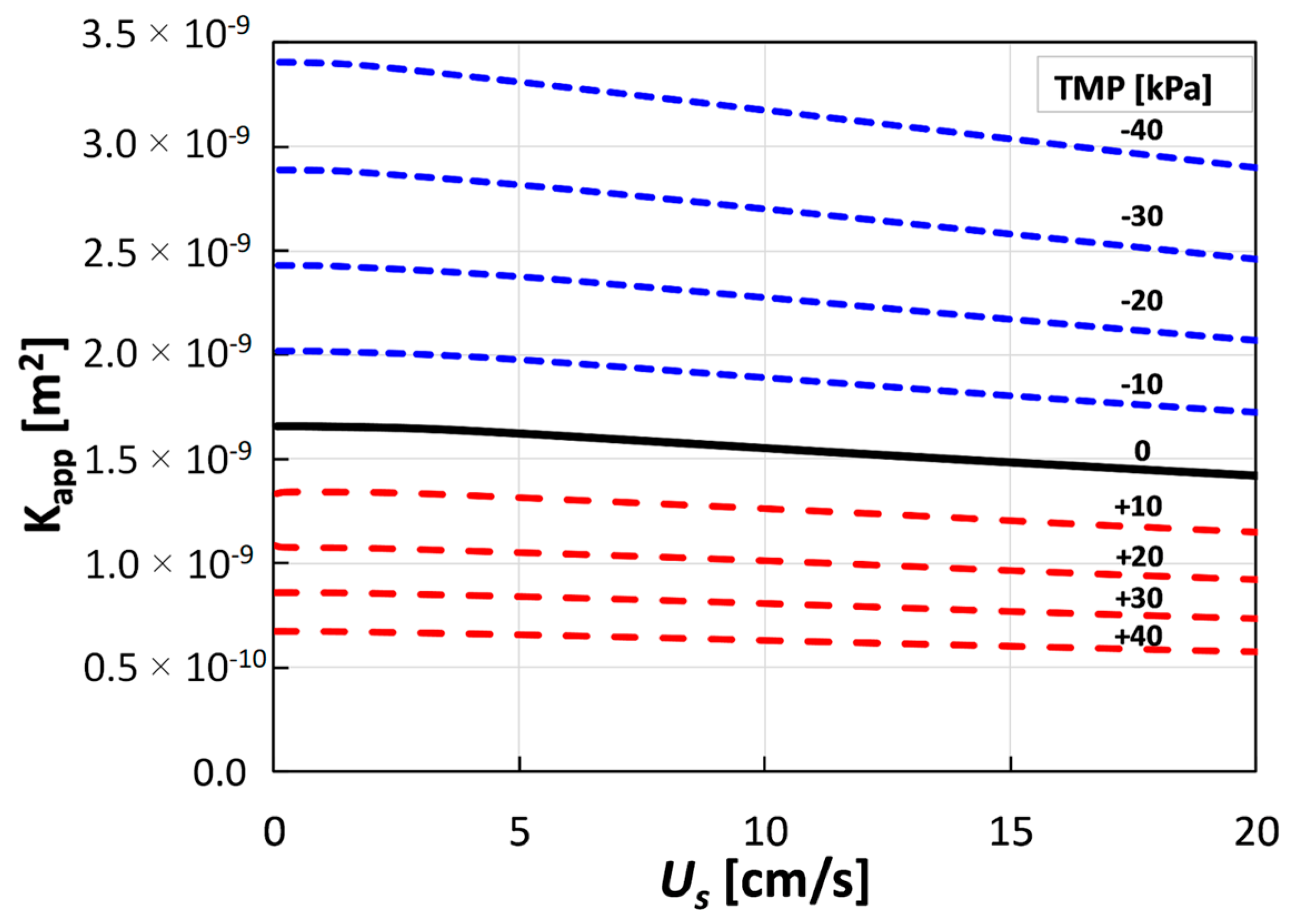
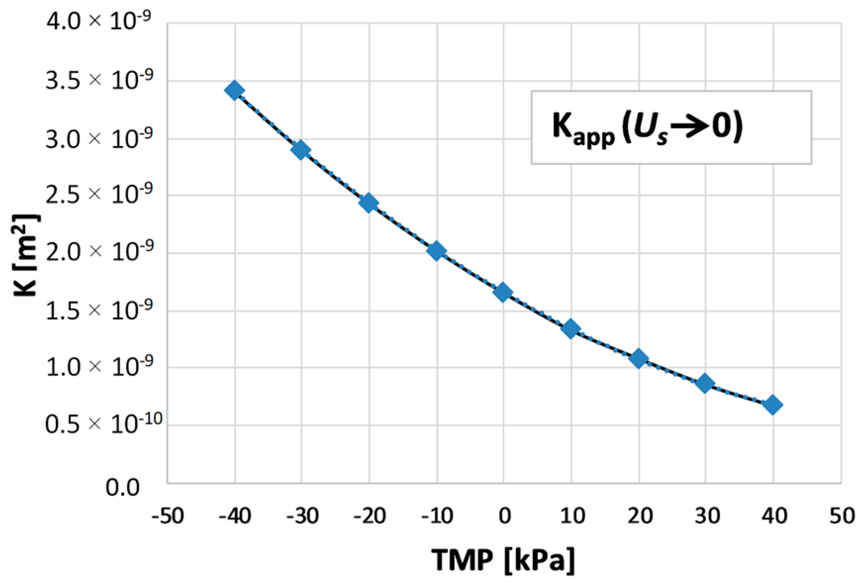
Appendix A.2. Channel Permeability for Non-Darcyan Flow

The slopes and intercepts of each linear segment of the piecewise linear fitting (discussed in Section 2.5) used to capture the dependence of the channel permeability on the velocity at different values of TMP are reported in Table A2 and Table A3.
Table A2. Slopes and intercepts for superficial velocity ranging between 0 and 7 cm/s.
0 < U < 3 cm/s3 < U < 7 cm/s
TMP [kPa]K [m2]a [cm/s]K′ [m2]a [cm/s]
406.754 · 10−1006.289 · 10−100.20677
308.651 · 10−1008.052 · 10−100.20784
201.088 · 10−901.012 · 10−90.20885
101.356 · 10−901.261 · 10−90.20938
01.670 · 10−901.553 · 10−90.20934
−102.034 · 10−901.891 · 10−90.20973
−202.439 · 10−902.271 · 10−90.20753
−302.893 · 10−902.693 · 10−90.20727
−403.397 · 10−903.163 · 10−90.20678
Table A3. Slopes and intercepts for superficial velocity ranging between 7 and 20 cm/s.
7 < U < 12 cm/s12 < U < 20 cm/s
TMP [kPa]K′ [m2]a [cm/s]K′ [m2]a [cm/s]
405.777 · 10−100.75985.169 · 10−101.9422
307.393 · 10−100.76346.612 · 10−101.9506
209.287 · 10−100.76688.302 · 10−101.9584
101.158 · 10−90.76861.034 · 10−91.9625
01.425 · 10−90.76841.274 · 10−91.9622
−101.735 · 10−90.76971.551 · 10−91.9651
−202.085 · 10−90.76231.865 · 10−91.9483
−302.473 · 10−90.76152.213 · 10−91.9462
−402.905 · 10−90.75982.600 · 10−91.9425

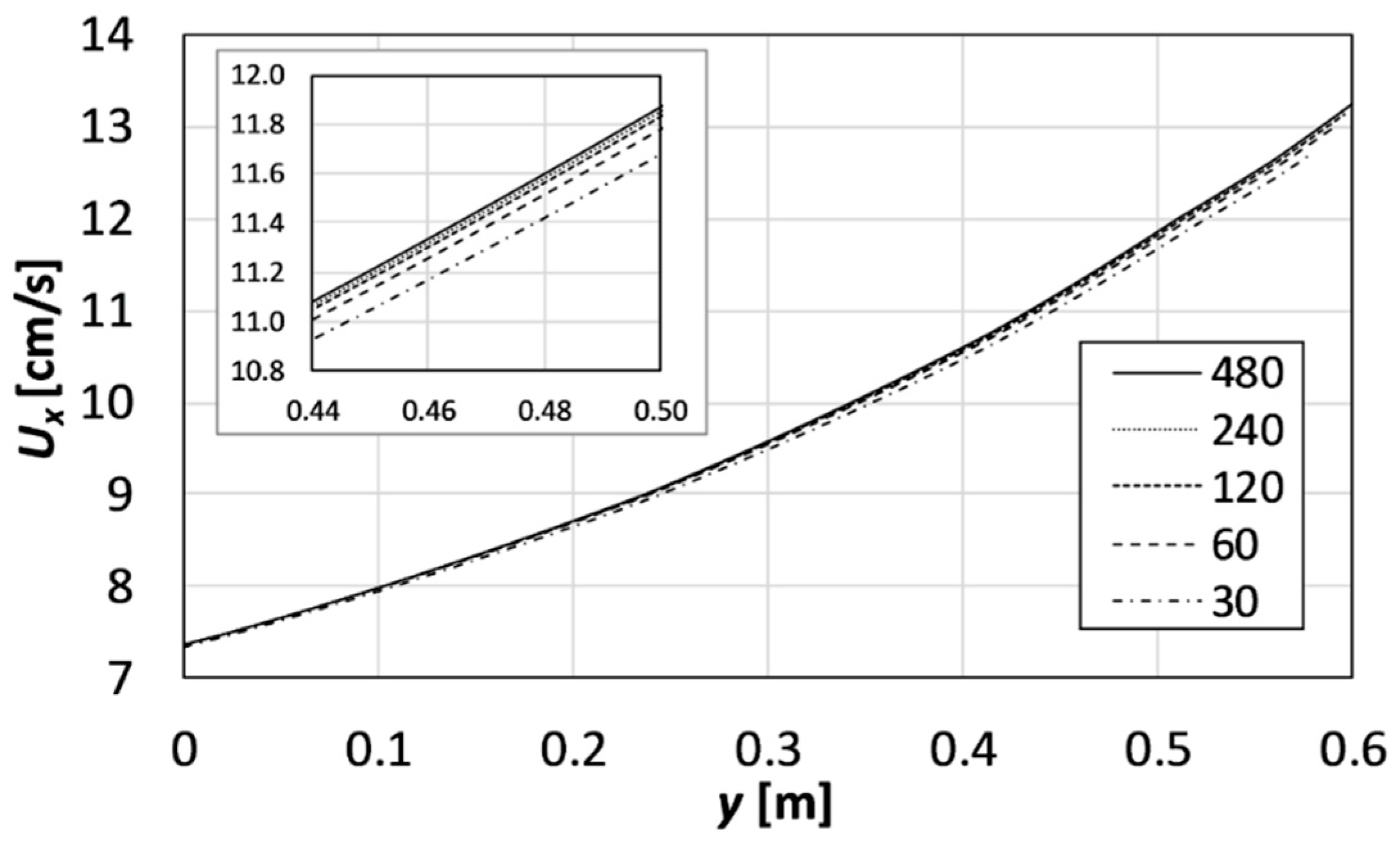
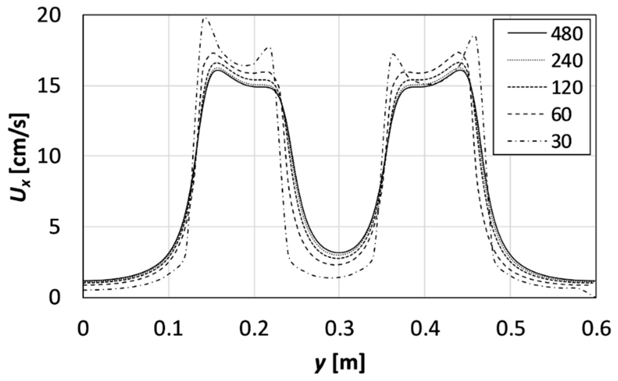
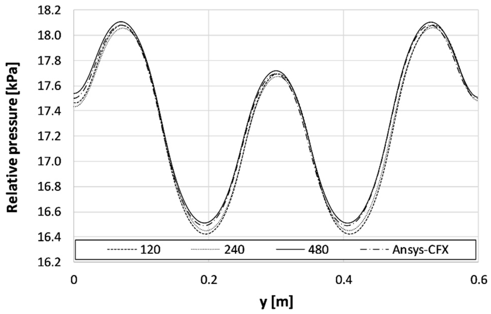
Appendix B. Grid Dependence and Validation Against CFD Results

Appendix B.1. Grid Dependence

As mentioned in Section 2.6, the effect of the number of channel divisions (Nx and Ny) on the model’s results was systematically addressed by comparing five grids characterized by: (A) 30 × 30; (B) 60 × 60; (C) 120 × 120; (D) 240 × 240; and (E) 480 × 480 blocks, with a total number of 900, 3600, 14,400, 57,600, and 230,400 blocks, respectively.
For the cross flow configuration at Pin = 34.3 kPa, Figure A1 reports profiles of the x-velocity component along a line orthogonal to the main flow direction and located 2 cm away from the inlet side; see the left broken line in Figure 8a. The inset shows an enlarged portion of the same plot. It can be observed that maximum differences (grids A vs. E) are less than 0.25 cm/s, and grids C–E yield practically identical results. The discrepancies between consecutive grids decrease with the number of blocks, indicating an asymptotic convergence.
Figure A1. Cross flow configuration at Pin = 34.3 kPa: profiles of the x-velocity component along a line orthogonal to the main flow direction and located 2 cm away from the inlet, see Figure 8a. Results obtained with five grids of increasing resolution are reported. The inset shows a magnified portion of the same plot.
Energies 12 04259 g0a1
A similar comparison for the counter flow configuration is reported in Figure A2, which shows profiles of the x-velocity component along a line orthogonal to the main flow direction and located 2 cm upstream of the outlet side; see the right broken line in Figure 8b. The maximum grid-dependent differences (grids A vs. E) are higher than for the cross flow case (up to ~4 cm/s) but are concentrated near the outflow slots. Grids C–E yield very similar results, with maximum differences of ~0.5 cm/s (~3%).
Figure A2. Counter flow configuration at Pin = 34.3 kPa: pressure profiles along a line orthogonal to the main flow direction and located 2 cm upstream of the outlet, see Figure 8b. Results obtained with five grids of increasing resolution are reported.
Energies 12 04259 g0a2
As far as the computing time is concerned, it typically increased from a few seconds for grid A to ~80 h for grid E when simulations were run on a desktop computer equipped with an Intel Core i7-6700 CPU with 32 GB memory. The computing time was significantly lower (about 50%) in the absence of deformation.

Appendix B.2. Comparison with CFD Results

The reliability of the present mathematical model formulation was verified by comparing the results for undeformed channel configurations (TMP = 0) with those provided by computational fluid dynamics (CFD) simulations. The commercial software Ansys CFX® 18.1 was employed. Both cross flow and countercurrent configurations were simulated. The CFD settings were as follows:
  • The porous media model was assumed, and steady state simulations were performed.
  • Values of the permeability and of the resistance loss coefficient were determined by means of a quadratic regression of the undeformed channel characteristics (Figure 6). The permeability was set to 1.65·10−9 m2 and the resistance loss coefficient to 989 m−1.
  • Free slip wall boundary conditions were set at the upper and lower walls of the channel (representative of membrane surfaces). The latter condition was imposed to avoid viscous fluid–wall interaction, which would lead to erroneous results; in fact, the friction characteristics of the membrane surfaces and profiles are already taken into account by the permeability and resistance coefficients.
  • Symmetry or no slip boundary conditions were imposed at the lateral edges of the domain.
CFD predictions for pressure and velocity were evaluated and compared with the results of the present model. For example, Figure A3 reports profiles of the relative pressure computed along a line orthogonal to the main flow direction and located 2 cm away from the inlet of a channel in the counter flow configuration at Pin = 18.64 kPa. Only the three finest grids, C, D, and E, were considered. It can be observed that the CFD predictions are practically coincident with the results provided by the finest grid (E, 480 × 480 blocks) but agree fairly well also with those obtained by coarser (120 × 120 or 240 × 240) grids. A similar agreement was also obtained for other locations, the other configuration (i.e., cross flow), and various flow velocities, thus confirming the reliability of the present model.
Figure A3. Single undeformed channel in the counter flow configuration at Pin = 18.64 kPa: pressure profiles along a line orthogonal to the main flow direction and located 2 cm away from the inlet, see Figure 8b. Results obtained with three grids of increasing resolution are compared with CFD predictions.
Energies 12 04259 g0a3

References

  1. Campione, A.; Gurreri, L.; Ciofalo, M.; Micale, G.; Tamburini, A.; Cipollina, A. Electrodialysis for water desalination: A critical assessment of recent developments on process fundamentals, models and applications. Desalination 2018, 434, 121–160. [Google Scholar] [CrossRef]
  2. Tufa, R.A.; Pawlowski, S.; Veerman, J.; Bouzek, K.; Fontananova, E.; di Profio, G.; Velizarov, S.; Goulão Crespo, J.; Nijmeijer, K.; Curcio, E. Progress and prospects in reverse electrodialysis for salinity gradient energy conversion and storage. Appl. Energy 2018, 225, 290–331. [Google Scholar] [CrossRef]
  3. Pawlowski, S.; Crespo, J.G.; Velizarov, S. Pressure drop in reverse electrodialysis: Experimental and modeling studies for stacks with variable number of cell pairs. J. Memb. Sci. 2014, 462, 96–111. [Google Scholar] [CrossRef]
  4. Pawlowski, S.; Rijnaarts, T.; Saakes, M.; Nijmeijer, K.; Crespo, J.G.; Velizarov, S. Improved fluid mixing and power density in reverse electrodialysis stacks with chevron-profiled membranes. J. Memb. Sci. 2017, 531, 111–121. [Google Scholar] [CrossRef]
  5. Gurreri, L.; Tamburini, A.; Cipollina, A.; Micale, G.; Ciofalo, M. CFD prediction of concentration polarization phenomena in spacer-filled channels for reverse electrodialysis. J. Memb. Sci. 2014, 468, 133–148. [Google Scholar] [CrossRef] [Green Version]
  6. La Cerva, M.; Liberto, M.D.; Gurreri, L.; Tamburini, A.; Cipollina, A.; Micale, G.; Ciofalo, M. Coupling CFD with a one-dimensional model to predict the performance of reverse electrodialysis stacks. J. Memb. Sci. 2017, 541, 595–610. [Google Scholar] [CrossRef] [Green Version]
  7. Pawlowski, S.; Geraldes, V.; Crespo, J.G.; Velizarov, S. Computational fluid dynamics (CFD) assisted analysis of profiled membranes performance in reverse electrodialysis. J. Memb. Sci. 2016, 502, 179–190. [Google Scholar] [CrossRef] [Green Version]
  8. Koutsou, C.P.; Yiantsios, S.G.; Karabelas, A.J. A numerical and experimental study of mass transfer in spacer-filled channels: Effects of spacer geometrical characteristics and Schmidt number. J. Memb. Sci. 2009, 326, 234–251. [Google Scholar] [CrossRef]
  9. Dirkse, M.H.; van Loon, W.K.P.; Stigter, J.D.; Post, J.W.; Veerman, J.; Bot, G.P.A. Extending potential flow modelling of flat-sheet geometries as applied in membrane-based systems. J. Memb. Sci. 2008, 325, 537–545. [Google Scholar] [CrossRef]
  10. Kostoglou, M.; Karabelas, A.J. On the fluid mechanics of spiral-wound membrane modules. Ind. Eng. Chem. Res. 2009, 48, 10025–10036. [Google Scholar] [CrossRef]
  11. Kostoglou, M.; Karabelas, A.J. Mathematical analysis of the meso-scale flow field in spiral-wound membrane modules. Ind. Eng. Chem. Res. 2011, 50, 4653–4666. [Google Scholar] [CrossRef]
  12. Kodým, R.; Vlasák, F.; Šnita, D.; Černín, A.; Bouzek, K. Spatially two-dimensional mathematical model of the flow hydrodynamics in a channel filled with a net-like spacer. J. Memb. Sci. 2011, 368, 171–183. [Google Scholar] [CrossRef]
  13. Pánek, P.; Kodým, R.; Šnita, D.; Bouzek, K. Spatially two-dimensional mathematical model of the flow hydrodynamics in a spacer-filled channel—The effect of inertial forces. J. Memb. Sci. 2015, 492, 588–599. [Google Scholar] [CrossRef]
  14. She, Q.; Hou, D.; Liu, J.; Tan, K.H.; Tang, C.Y. Effect of feed spacer induced membrane deformation on the performance of pressure retarded osmosis (PRO): Implications for PRO process operation. J. Memb. Sci. 2013, 445, 170–182. [Google Scholar] [CrossRef]
  15. Karabelas, A.J.; Koutsou, C.P.; Sioutopoulos, D.C. Comprehensive performance assessment of spacers in spiral-wound membrane modules accounting for compressibility effects. J. Memb. Sci. 2018, 549, 602–615. [Google Scholar] [CrossRef]
  16. Hereijgers, J.; Ottevaere, H.; Breugelmans, T.; De Malsche, W. Membrane deflection in a flat membrane microcontactor: Experimental study of spacer features. J. Memb. Sci. 2016, 504, 153–161. [Google Scholar] [CrossRef]
  17. Moreno, J.; Slouwerhof, E.; Vermaas, D.A.; Saakes, M.; Nijmeijer, K. The Breathing Cell: Cyclic Intermembrane Distance Variation in Reverse Electrodialysis. Environ. Sci. Technol. 2016, 50, 11386–11393. [Google Scholar] [CrossRef]
  18. Park, S.-M.; Lee, S. Influence of Hydraulic Pressure on Performance Deterioration of Direct Contact Membrane Distillation (DCMD) Process. Membranes 2019, 9, 37. [Google Scholar] [CrossRef]
  19. Lian, B.; Blandin, G.; Leslie, G.; Le-Clech, P. Impact of module design in forward osmosis and pressure assisted osmosis: An experimental and numerical study. Desalination 2018, 426, 108–117. [Google Scholar] [CrossRef]
  20. Yuan, Z.; Wei, L.; Afroze, J.D.; Goh, K.; Chen, Y.; Yu, Y.; She, Q.; Chen, Y. Pressure-retarded membrane distillation for low-grade heat recovery: The critical roles of pressure-induced membrane deformation. J. Memb. Sci. 2019, 579, 90–101. [Google Scholar] [CrossRef]
  21. Hong, S.K.; Kim, C.S.; Hwang, K.S.; Han, J.H.; Kim, H.K.; Jeong, N.J.; Choi, K.S. Experimental and numerical studies on pressure drop in reverse electrodialysis: Effect of unit cell configuration. J. Mech. Sci. Technol. 2016, 30, 5287–5292. [Google Scholar] [CrossRef]
  22. Battaglia, G.; Gurreri, L.; Airò Farulla, G.; Cipollina, A.; Pirrotta, A.; Micale, G.; Ciofalo, M. Membrane Deformation and Its Effects on Flow and Mass Transfer in the Electromembrane Processes. Int. J. Mol. Sci. 2019, 20, 1840. [Google Scholar] [CrossRef] [PubMed]
  23. Battaglia, G.; Gurreri, L.; Airò Farulla, G.; Cipollina, A.; Pirrotta, A.; Micale, G.; Ciofalo, M. Pressure-Induced Deformation of Pillar-Type Profiled Membranes and Its Effects on Flow and Mass Transfer. Computation 2019, 7, 32. [Google Scholar] [CrossRef]
  24. Ciofalo, M.; Ponzio, F.; Tamburini, A.; Cipollina, A.; Micale, G. Unsteadiness and transition to turbulence in woven spacer filled channels for Membrane Distillation. J. Phys. Conf. Ser. 2017, 796, 012003. [Google Scholar] [CrossRef]
  25. Schock, G.; Miquel, A. Mass transfer and pressure loss in spiral wound modules. Desalination 1987, 64, 339–352. [Google Scholar] [CrossRef]
  26. Irmay, S. On the theoretical derivation of Darcy and Forchheimer formulas. Eos Trans. Am. Geophys. Union 1958, 39, 702–707. [Google Scholar] [CrossRef]
  27. Strathmann, H. Electrodialysis, a mature technology with a multitude of new applications. Desalination 2010, 264, 268–288. [Google Scholar] [CrossRef]
  28. Tedesco, M.; Mazzola, P.; Tamburini, A.; Micale, G.; Bogle, I.D.L.; Papapetrou, M.; Cipollina, A. Analysis and simulation of scale-up potentials in reverse electrodialysis. Desalin. Water Treat. 2014, 55, 3391–3403. [Google Scholar] [CrossRef] [Green Version]
  29. Moreno, J.; Grasman, S.; Van Engelen, R.; Nijmeijer, K. Upscaling Reverse Electrodialysis. Environ. Sci. Technol. 2018, 52, 10856–10863. [Google Scholar] [CrossRef] [Green Version]
  30. Wright, N.C.; Shah, S.R.; Amrose, S.E.; Winter, A.G. A robust model of brackish water electrodialysis desalination with experimental comparison at different size scales. Desalination 2018, 443, 27–43. [Google Scholar] [CrossRef]
Figure 1. A channel delimited by profiled membranes of the overlapped crossed filaments (OCFs) type. A repetitive periodic unit (“unit cell”) is shown, enlarged, in the inset. The geometric parameters H (channel thickness), P (pitch), and γ (flow attack angle) are indicated. Adapted from [22].
Energies 12 04259 g001
Figure 2. Sketch of a cell pair with diluate (DIL) and concentrate (CON) channels. Membranes are shown only for the sake of clarity but are not part of the computational domain. The bottom row reports a representation of the computational “molecules” adopted for the formulation of discrete balance equations in both channels.
Energies 12 04259 g002
Figure 3. Apparent permeability, Kapp, of the concentrate channel as a function of the equivalent velocity, U s , at different values of the transmembrane pressure for OCF-profiled membranes with P/H = 8, computed by 3-D mechanical-CFD simulations [22].
Energies 12 04259 g003
Figure 4. Permeability, K, at Us → 0 as a function of transmembrane pressure for OCF-profiled membranes with P/H = 8, computed by 3-D mechanical CFD simulations [22].
Energies 12 04259 g004
Figure 5. Flowchart of the iterative algorithm for the case of low velocity.
Energies 12 04259 g005
Figure 6. Dependence of the superficial velocity on the pressure gradient for the undeformed channel case (solid blue line), computed by 3-D CFD simulations [22]. The dotted red line represents the linear relation valid at low velocities. The straight red segments separated by symbols represent a piecewise linear fitting. As an example, the intercept, a, and the slope, K’/μ, of the fourth segment are indicated.
Energies 12 04259 g006
Figure 7. Algorithm flowchart in the case of non-Darcyan flow regime.
Energies 12 04259 g007
Figure 8. The flow arrangements analyzed in the present work. (a) cross flow; (b) counter flow. The insets in the top row show the actual geometry of inlets and outlets. The second and third rows report the approximated geometry simulated here that apply to the two solutions (e.g., concentrate and diluate). The broken lines in the middle graphs are those along which the velocity and pressure profiles obtained with different grids were compared (Appendix B).
Energies 12 04259 g008
Figure 9. Results for a cross flow stack of 0.6 m sides at PinPout = 3.12 kPa (Us = 1 cm/s) in the absence of membrane deformation: relative pressure maps for the CON (a) and DIL (b) channels, and TMP (c).
Energies 12 04259 g009
Figure 10. Results for a cross flow stack of 0.6 m sides at PinPout = 3.12 kPa (Us ≈ 1 cm/s) in the presence of membrane deformation: relative pressure maps for the CON (a) and DIL (b) channels, TMP (c), and concentrate channel equivalent height (d), superficial velocity components along the x (e) and y (f) directions, and interstitial velocity along the x direction (g).
Energies 12 04259 g010
Figure 11. Results for a cross flow stack of 0.6 m sides at PinPout = 34.3 kPa (Us = 10 cm/s) in the absence of membrane deformation: relative pressure maps for the CON (a) and DIL (b) channels, and TMP (c).
Energies 12 04259 g011
Figure 12. Results for a cross flow stack of 0.6 m sides at PinPout = 34.3 kPa (Us ≈ 10 cm/s) in the presence of membrane deformation: relative pressure maps for the CON (a) and DIL (b) channels, TMP (c), and concentrate channel equivalent height (d), superficial velocity components along the x (e) and y (f) directions, and interstitial velocity along the x direction (g).
Energies 12 04259 g012
Figure 13. Results for a cross flow stack of 0.6 m sides at PinPout = 34.3 kPa (Us ≈ 10 cm/s) in the presence of membrane deformation: profiles of TMP (a), and concentrate channel equivalent height (b), apparent permeability (c), pressure gradient (d), superficial velocity (e) and interstitial velocity (f) along the x direction at y = 0.05 and 0.55 m. Corresponding results would be obtained for the diluate channel.
Energies 12 04259 g013
Figure 14. Pressure profiles along the x-direction near the lower edge (y = 0.55 m) of the concentrate channel for the cross flow configuration and 〈Us〉 ≈ 1, 5, and 10 cm/s. Profiles are reported both in the presence and absence of membrane deformation.
Energies 12 04259 g014
Figure 15. Results for a cross flow stack of 0.6-m sides at PinPout = 34.3 kPa (〈Us〉 = 8.5 cm/s) in the absence of membrane deformation: maps of relative pressure in the CON (a) and DIL (b) channels, TMP (c), and superficial velocity along the x direction in the concentrate channel (d).
Energies 12 04259 g015
Figure 16. Results for a cross flow stack of 0.6-m sides at 〈Us〉 = 7.5 cm/s in the presence of membrane deformation: maps of relative pressure in the CON (a) and DIL (b) channels; TMP (c); and channel equivalent height (d), superficial velocity (e), and interstitial velocity (f) along the x direction in the concentrate channel.
Energies 12 04259 g016

