Improving Prediction Intervals Using Measured Solar Power with a Multi-Objective Approach


Computer Science Department, Universidad Carlos III de Madrid, 30 Avenida Universidad, Leganes, 28911 Madrid, Spain
*
Author to whom correspondence should be addressed.
Energies 2019, 12(24), 4713; https://doi.org/10.3390/en12244713
Submission received: 25 October 2019
/
Revised: 27 November 2019
/
Accepted: 5 December 2019
/
Published: 10 December 2019
(This article belongs to the Special Issue Applications of Artificial Intelligence in Renewable Energy)
Abstract
:Prediction Intervals are pairs of lower and upper bounds on point forecasts and are useful to take into account the uncertainty on predictions. This article studies the influence of using measured solar power, available at prediction time, on the quality of prediction intervals. While previous studies have suggested that using measured variables can improve point forecasts, not much research has been done on the usefulness of that additional information, so that prediction intervals with less uncertainty can be obtained. With this aim, a multi-objective particle swarm optimization method was used to train neural networks whose outputs are the interval bounds. The inputs to the network used measured solar power in addition to hourly meteorological forecasts. This study was carried out on data from three different locations and for five forecast horizons, from 1 to 5 h. The results were compared with two benchmark methods (quantile regression and quantile regression forests). The Wilcoxon test was used to assess statistical significance. The results show that using measured power reduces the uncertainty associated to the prediction intervals, but mainly for the short forecasting horizons.

1. Introduction
In the last decade, wind and solar energy production, and more specifically photovoltaic (PV) energy, has increased significantly and, therefore, a large PV penetration with a rapid growth has taken place in the electricity market [1]. To achieve this high penetration, it is important to have accurate point forecasts and most of the research has focused on this issue. However, due to the high variability of several meteorological factors, solar power prediction is inherently uncertain and, therefore, it is also important to estimate the uncertainty around point forecasts. Accurate knowledge of uncertainty on renewable energy production can provide both economic opportunities [2] and reliability improvement [3]. Recent literature shows how research into new uncertainty estimation methods, as well as their applications to the renewable energy industry, is a field of great activity [4,5,6].
The most commonly used ways of representing uncertainty are quantiles and prediction intervals (PIs). The estimation of quantiles has been widely addressed in the literature, especially through methods that estimate each desired quantile independently. For example, quantile regression () [7] constructs linear models by minimizing quantile loss (or pinball score) for a particular quantile-probability. Nonlinear models can also be constructed using this cost function, for example quantile regression neural networks () [8] or tree-based ensembles such as Gradient Tree Boosting () [9,10]. There are also techniques which build a single model from which all quantiles can be extracted. For instance, quantile regression forests () [11] is another non-linear ensemble technique and analog ensembles (AnEn) [12,13,14] generate probability distributions using a set of past measurements that correspond to the most similar past numerical weather prediction (NWP) forecasts to the current situation.
Another way of representing forecast uncertainty is by means of PIs, where two bounds, lower and upper, contain the actual value with a given probability (called prediction interval probability coverage (PICP)) [15]. For a given PICP, the narrower is the PI, the less uncertain is the forecast. There are in the literature many classic methods for computing PIs [16], but, more recently, an evolutionary approach, known as LUBE (lower upper bound estimation), has shown better performance in several domains [16], including renewable energy forecasting [17,18]. The approach uses a two-output artificial neural networks, for the lower and upper bounds of the interval, respectively. For point forecasting, the actual output to the networks is available, and, thus, supervised training techniques, such as backpropagation can be used. However, this is not the case for LUBE, because the two outputs of the network (i.e., the lower and upper bounds) are not directly available. For this reason, the network parameters are usually optimized using evolutionary computation techniques such as simulated annealing (SA) [19] or particle swarm optimization (PSO) [20]. Optimizing PIs is clearly a multi-objective problem, because obtaining high-coverage but narrow intervals are conflicting goals. However, most LUBE approaches translate the multi-objective problem into a single-objective one, by aggregating the two goals, but this requires some reasonable weighting between the objectives to be decided in advance. LUBE can also be addressed as an actual multi-objective approach that does not require goal weighting. This was the approach proposed by the authors in a previous work [21], where a multi-objective particle swarm optimization evolutionary algorithm (MOPSO) showed very good performance in a solar energy production forecasting problem on Oklahoma solar sites [22], where only meteorological forecasts were used as input. An important advantage of using a multi-objective algorithm is that in a single run the method is able to return a whole set of solutions (Pareto front), which represent the best trade-offs between coverage and width, out of which the user can select a solution for some particular coverage.
Most works that deal with energy prediction use meteorological forecast variables as inputs for the prediction models. However, some articles indicate that prediction error can be improved by using actual measurements available at prediction time, in addition to meteorological forecasts [23,24]. For instance, a solar plant that, at time , needs to issue a power output forecast for the next hour () can apply a model that uses (as inputs) meteorological forecasts for as well as the current power output (measured at ). Martín-Vázquez et al. [25] showed that, in fact, the use of measured output wind electrical power was helpful to improve point forecasts for short horizons in wind energy forecasting. However, not much research has been done to study the influence of using measurements for constructing PIs, although preliminary results point in that direction [26].
The purpose of this article is to study whether the quality of PIs for PV power forecast can be improved by using measured solar output power in addition to meteorological forecast variables. Given that it could be expected that measurements at may influence short horizons more strongly than longer ones, in this work, several forecast horizons are considered. In principle, using measured information at prediction time should reduce the uncertainty of forecasts (and, therefore, PIs should be narrower), but this advantage is expected to decrease for long prediction horizons. Thus, the main contributions of this article are to study both the degree of improvement of PIs when using measured information and the dependency of that improvement on the prediction horizon. We used the LUBE approach optimized with [21]. The approach has already been used for estimating PIs for the aggregated daily energy production forecast for next day [21]. However, in the context of solar forecasting, it is also important to provide uncertainty forecasts for intra-day horizons, which is what we do in the current work. We also used for comparison purposes two benchmark methods recommended in recent literature for probabilistic solar forecasting [4]. The first is [7], a commonly used linear method for obtaining quantiles in solar forecasting [27]. The second one is [11], a non-linear method successfully used in recent works on solar energy uncertainty estimation [28,29]. All methods were tested using as inputs only the meteorological variables and using the meteorological variables together with measured solar power at .
The study was done using data from the Global Energy Forecasting Competition 2014 (GEFCom2014) concerning the probabilistic solar power forecasting problem [30]. To advance beyond the preliminary results [26], in this study, extensive experimentation was carried out. Data from three different solar plants in Australia (Stations 1–3) were used and the PIs were estimated for five intra-day forecasting horizons (1–5 h, UTC time). Given that and are stochastic techniques, they were run 90 times and statistical tests for comparison were done by means of the Wilcoxon test. The extensiveness of the experiments and the statistical test allowed extracting reliable conclusions.
The rest of the article is organized as follows. Section 2 describes the dataset used for experiments. Section 3 summarizes the evolutionary multi-objective approach for interval optimization. Section 4 describes the two baseline methods for comparison. Section 5 describes the experimental setup and the results, including statistical significance tests. Conclusions are finally drawn in Section 6.
2. Data Description
The data used in this work were obtained from Task 15 in the probabilistic solar power forecasting problem [30] one of the four tracks from the Global Energy Forecasting Competition 2014 (GEFCom2014). These data include measured solar power generation and meteorological forecasts for three solar stations (Stations 1–3) in Australia whose exact location was been revealed. Measured solar power generation, expressed in proportions between 0 and 1 relative to the nominal power of the plant, was provided hourly, from 1 April 2012 01:00 to 1 July 2014 00:00 UTC. The meteorological forecasts were obtained from the European Centre for Medium-range Weather Forecasts (ECMWF) and include 12 weather variables. Forecasts for those weather variables are issued by ECMWF once per day, at midnight, and they are forecasted for the each hour for the next 24 h. Thus, if is the time at which forecasts are issued (00:00 UTC), each meteorological variable gets a forecast for , , …, .
The 12 weather variables are: total column liquid water, i.e., the vertical integral of cloud liquid water content (kg · m); total column ice water, i.e., the vertical integral of cloud ice water content (kg · m); surface pressure (Pa); relative humidity with respect to saturation at 1000 mbar; total cloud cover (0–1); 10-m U wind component (m · s); 10-m V wind component (m · s); 2-m temperature (K); surface solar radiation downward (J · m); surface thermal radiation downward (J · m); top net solar radiation, i.e., net solar radiation at the top of the atmosphere (J · m); and total precipitation (convective precipitation + stratiform precipitation) (m).
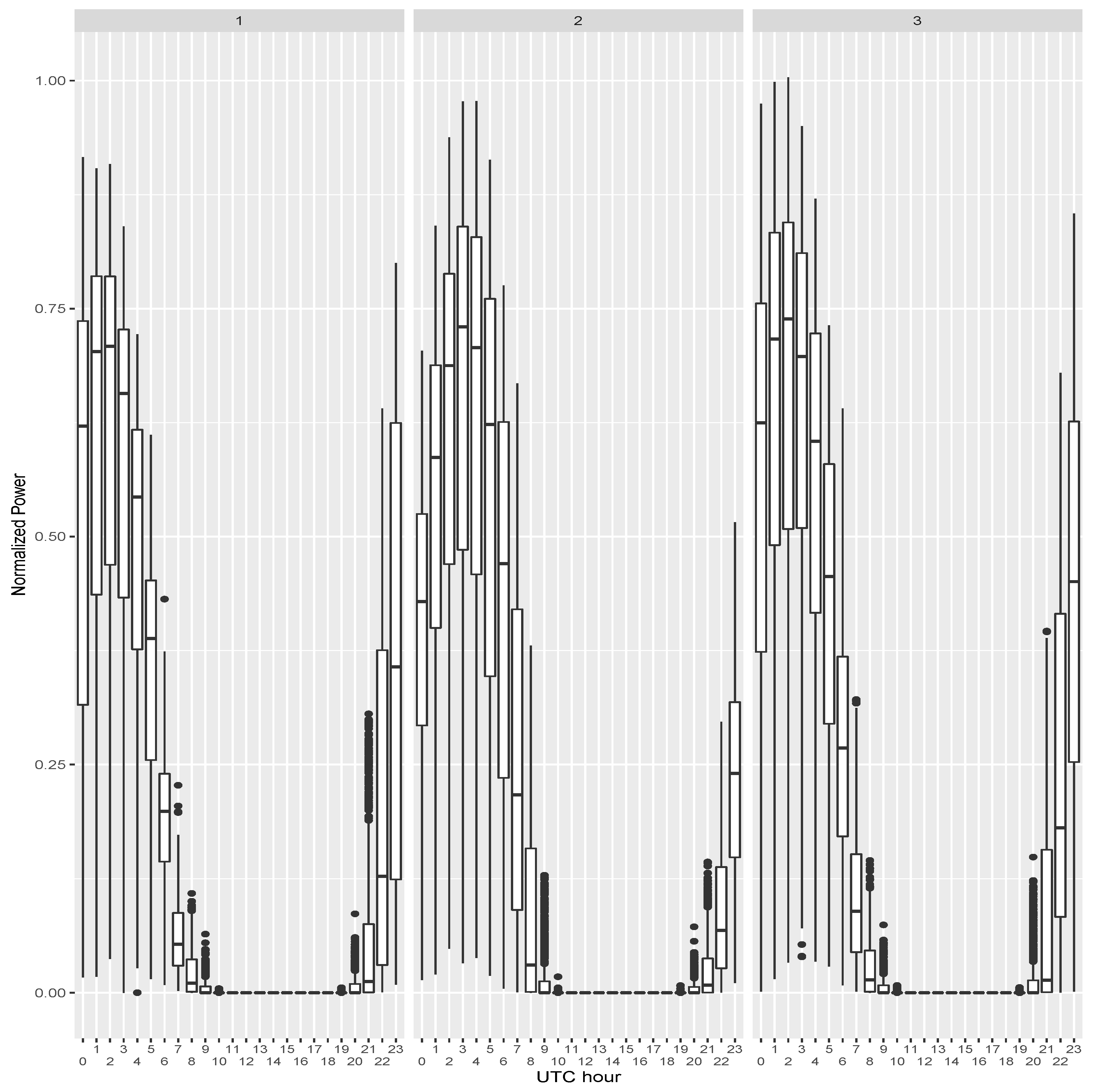
Figure 1 displays a box plot of the normalized measured power generation for each station corresponding to the whole period (2012-04-01 01:00 to 2014-07-01 00:00) and broken down by UTC hour. It is a standard box plot where the lower and upper hinges correspond to the first and third quartiles and the center black horizontal bar is the median. Whiskers are used to denote data in the 1.5*inter-quartile range and black points are used for outliers. It is important to remark that the hour on the x-axis corresponds to EMCWF time. Given that GEFCom2014 did not disclose the actual location of the three solar stations, it is not possible to know with certainty the local time for each of the stations. It is estimated that noon must correspond to the maximum of solar radiation (Time 1–2 for Station 1; Time 3 for Station 2; and Time 2 for Station 3). Zero is the hour at which ECMWF forecasts are issued. Based on the box plot in Figure 1, and given that measured power should be expected to have influence mostly for short time horizons, it was decided to study Hours 1–5. This also excludes hours too close to the night period.
Given that, for each horizon, there is a single forecast everyday, the available data are made of 820 instances, corresponding to 820 days. To ensure that both train and test sets are representative, every 30 days, 20 consecutive days were chosen for training and the remaining 10 for testing. Therefore, there were 550 days for training and 270 days for testing. To perform hyper-parameter tuning tasks, such as choosing the best neural network architecture, the best number of optimization iterations or the best configuration for , it is necessary to split the available training data into another two sets: the training set and the validation set (also known as the development (dev) set). In this work, for every 20-day block of the original training partition, the first 14 days were finally used for training, and the remaining six for validation.
3. Multi-Objective Optimization for Prediction Intervals
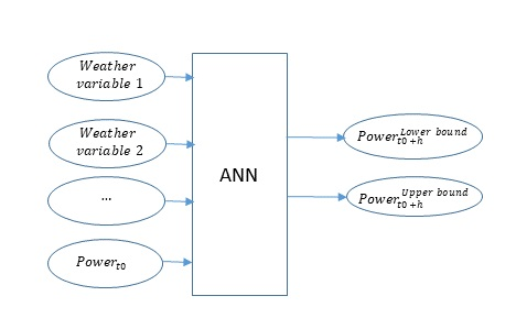
The following section describes the multi-objective particle swarm optimization algorithm () applied to PI, originally reported in [21]. This application was inspired by LUBE [16], which used an artificial neural network (ANN) with a single hidden layer to make an estimation of the lower and upper bounds of the PIs. The ANN was optimized using multi-objective evolution techniques.
In this study, the inputs to the ANN can be meteorological forecast variables and measured solar output power. The outputs of the network are the boundaries (lower and upper) forecasted with the network for the given inputs. For each input in the dataset, an observation of power is found. However, the boundaries are never included, therefore a backpropagation optimization is not suitable for this network. As the desired outputs are unknown, this is not a standard supervised regression, and an alternative optimization technique is required.
Therefore, an evolutionary optimization algorithm was chosen to optimize the weights of the network with two primary goals: PI coverage and interval width. Coverage is measured using the prediction interval coverage probability (), which computes the frequency of observations laying within the interval. The PICP can be maximized by also maximizing the width of the PI, producing trivial solutions. To avoid this, a second goal was set to minimize the width of the PI. The following paragraphs formalize the formulation of these goals.
Let be a set of observations, where is a vector with the input variables and is the observed output variable. Let be the prediction interval for observation ( are the outputs of the ANN). The goal can be calculated as described in Equation (1) and the average interval width () in Equation (2).
where N is the number of samples, is the indicator function for interval (it is 1 if and 0 otherwise), and and represent the PI boundaries.
Optimizing requires sacrificing a higher , while a narrow will lose some coverage in return. The goals are opposed and a multi-objective approach was applied [21]. Every particle in the represents a single solution to the network, i.e., a different configuration of weights. The goals of this algorithm are: (Equation (1)) and (Equation (2)). This network receives the meteorological data (from the given dataset in Section 2) as inputs and measured solar power at .
The algorithm produces a set of multiple ANNs laid in a Pareto front of non-dominated solutions. Typically, PIs with a desired coverage, called PIs’ nominal coverage (or ), are needed by the user. Sometimes, it is more appropriate to refer to , which is named as from now on. In this approach, the solution in the Pareto front with closest to the one requested by the user is selected [21].
4. Benchmark Methods
4.1. Quantile Regression
The [7] algorithm is able to forecast quantiles by using linear models. In comparison, the least squares method makes a prediction of the target conditional average, while predicts the median or other quantiles. This is done by minimizing the quantile loss instead of the quadratic loss. Quantiles can be used for obtaining PIs. Let and be the and quantiles, respectively. There are two quantiles and for the left and right probability tails of the distribution, respectively. The coverage of the PI is equal to . To summarize, builds a couple of linear models to estimate the and quantiles, forming the PI in turn.
4.2. Quantile Regression Forest
[11] is an adaption of the random forest () algorithm [31] for estimating quantiles and follows a different strategy to linear quantile regression. RF is an ensemble learning algorithm whose individual models are regression trees. Each of the trees is obtained from different subsets of the training data by means of bootstrap sampling. To obtain an output for an instance, it is dropped down the tree until it reaches a leaf. The average of the response value of the training instances in the leaf is returned. RF can become by first adapting the regression trees by changing the information that is stored in the leaf nodes. In the case of , leaf nodes store not only the average response, but all the response values of the training instances that reached the leaf. When an instance is dropped down each of the trees in the ensemble, every regression tree returns a set of response values (the ones in the leaves reached by the instance). From the union of all these response values, quantiles can be estimated. PIs can be computed from the quantiles, similar to what was done with quantile regression.
5. Experimental Validation
and the two benchmark approaches ( and ) were evaluated to construct PIs for the study case described in Section 2. The main comparison refers to using and not using the power measures at . The latter is identified as . Therefor, six configurations were tested: , , , , , and . PIs obtained from the different approaches were evaluated using two metrics: average interval width () and ratio (obtained as ). The larger is the ratio, the better is the trade-off between and . Solutions that reach large with wide intervals are penalized with small ratio values.
PIs were obtained independently for each of the five forecast horizons (1–5 h). Several target nominal coverage values () were considered within the range 0.02–0.20. and approaches must be run for each desired value. The approach is able to obtain PIs for all in a single run (see Section 3). Ninety runs were executed for (each run was valid for all the values) and because they are stochastic methods. For , only one run for each was executed, because it is not stochastic. The following three subsections describe the tuning of the hyper-parameters of the methods, the experimental results, and the statistical significance tests.
5.1. Hyper-Parameter Tuning
Two hyper-parameters were tuned for : number of hidden neurons and number of iterations of PSO. The methodology used a training and validation set approach, where the validation set was used to compare and select the best hyper-parameter values. The values of hidden neurons explored were: 2, 4, 6, 8, 10, 15, 20, 30, and 50. The different values for the PSO iterations ranged from 1000 to 16,000 in steps of 1000. Ninety runs were carried out for each number of neurons and iterations, starting with different random seeds. Therefore, each of the 90 runs had its own hyper-parameter tuning process, which resulted in an optimal number of neurons and iterations for each run. The optimal hyperparameters were chosen using the validation set hypervolume ([21]). It is important to remark that this parameter optimization process was carried out independently for each of the five forecasting horizons. The 90-run average (and standard deviation) of the best hyper-parameters for each horizon and configuration ( and ) is displayed in Table 1.
It is observed that the number of hidden neurons depends on the horizon, and long horizons seem to require fewer hidden neurons than short horizons. This trend is not systematic, but it is true for all stations and horizons that more neurons are required for the first hour than for the fifth hour. A possible explanation is that, for longer horizons, predictions are more noisy, and simpler models are required to avoid overfitting. In any case, it shows that tuning the number of neurons separately for each horizon is useful. The number of iterations is always between 12,000 and 14,000, below the maximum value of 16,000, which shows that the iteration limit was appropriate. Nevertheless, we tried increasing this value for a few runs, but no significant changes in the Pareto fronts were observed.
For , no parameter tuning is required. However, the performance of RF method depends on two main parameters: nodesize (minimum number of samples in the tree leaves) and mtry (number of input attributes used en the trees). Therefore, for , we also performed hyper-parameter tuning to select the most suitable configuration. The values explored for nodesize were 2, 5, 10, 20, 30, 40, 50, and 100 and for mtry 2, 4, 6, 8, 10, 12, and 14 (the last one only when past value of power () was used as input). The measure used for selecting the best combination of parameters for was the ratio in the validation set. The study of best parameters was also carried out for each prediction horizon, as for approach. In this case, values of the parameters are very similar for the three stations, the five forecasting horizons, and the different target values. Nodesize values are around with no past power and around when was used. For mtry, the average values are around when no past power was used and when was used (bearing in mind that, when past power was used, an additional attribute was added to the set of inputs).
5.2. Experimental Results
To have a first view of the performance of the different methods, Table 2 shows the mean of the ratio values for each method and each horizon, separately for Stations 1–3. Each ratio value is the mean of the ratios for all the values (0.02, 0.05, 0.08, 0.1, 0.15, and 0.2).
The results show that obtains better results than for the nearest horizons (especially Horizons 1 and 2) and for the three locations. For the other methods ( and ), the variant also behaves better than the original method, and this situation occurs for all the prediction horizons and all the stations. Comparing with the other methods, we can observe that, for all horizons and stations, it obtains higher ratio values. When we compare and methods, we can observe that there is not a clear predominance of any method. In some cases, the ratio values of are better (Station 1), but, in other cases, it is the opposite, as in Station 3. Next, the results are analyzed in more detail.
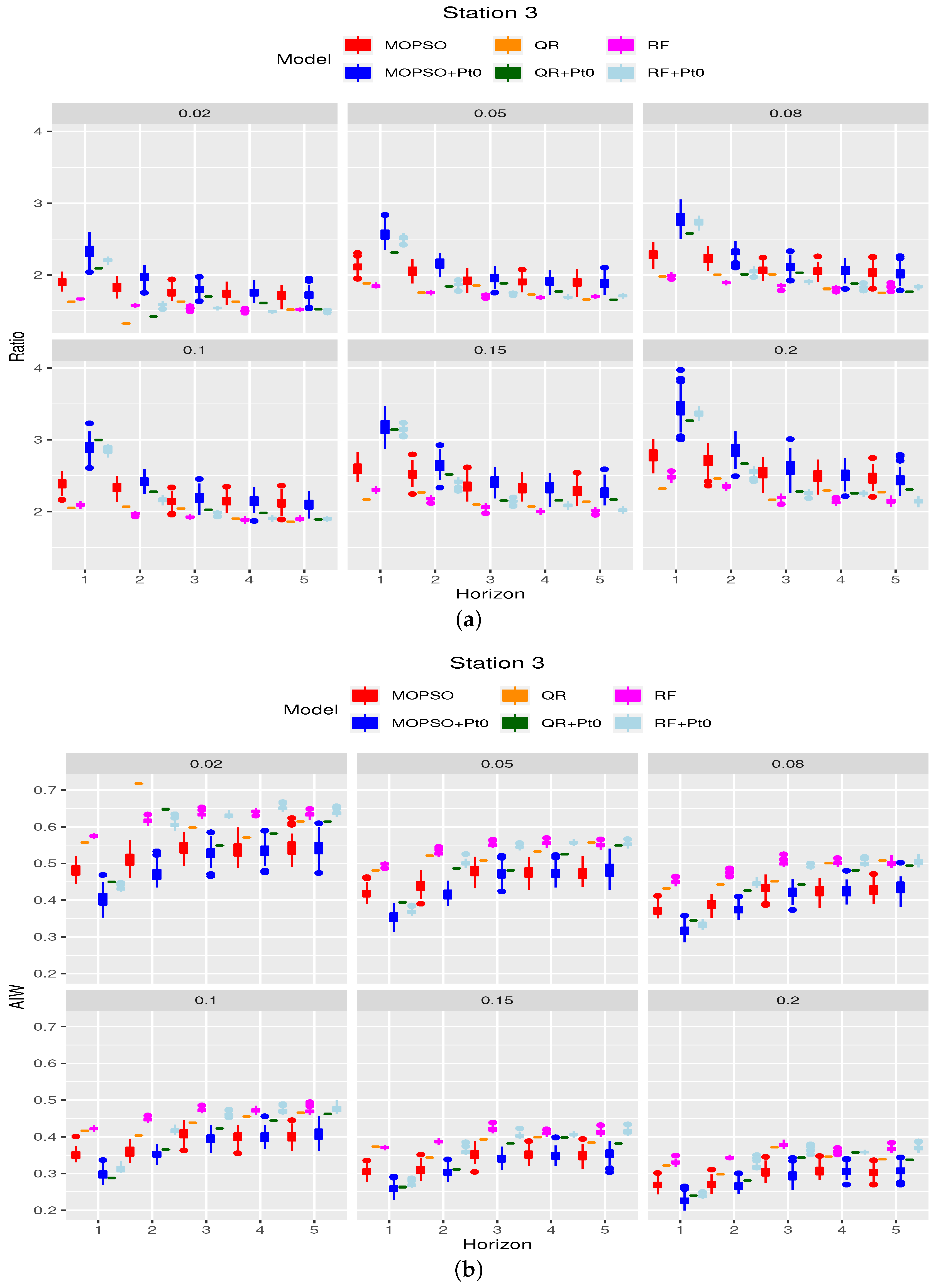
Figure 2, Figure 3 and Figure 4 display the results (ratio and ) for each of the three stations, respectively. Each of the figures contain two plots, top for the ratio (a) and bottom for (b). These figures compare , , , , , and . Information for , , , and is displayed by means of box plots, because they are a good summary of the 90 runs. and are shown as horizontal lines, because is not stochastic. Plots can be seen for some representative values (0.02, 0.05, 0.08, 0.1, 0.15, and 0.2). Figure 2a displays the ratio of the six methods tested for Station 1. It is readily apparent that ratio of is larger than for the first horizon, and, to a lesser degree, for the second one. This should be expected, because the influence of measures at time should decrease as the horizon is farther away from . It can also be noticed that the difference between and decreases as increases. For instance, for the second horizon, is clearly better than for but quite similar for . The second issue to notice in Figure 2 is that, although and also benefit from using at short horizons, configurations typically outperform their and counterparts (i.e., ’s ratio is larger than those of and , and it also is when is not used). This is true for all horizons and s. The plot on the bottom of Figure 2b confirms the previous findings: intervals are narrower than for the first two horizons (and that is also true for , , , and ), highlighting the importance of using for obtaining narrow intervals. Again, configurations always obtain narrower intervals than the and baselines. Figure 3 supports the previous results for Station 2. In this case, higher ratios are obtained by (vs. , and ) for longer horizons (from 1 to 4 h). Finally, those results are mirrored by Station 3, as shown in Figure 4, although in this case there is an anomaly for = 0.1, where manages to obtain better ratios (and narrower intervals) than for the first forecasting horizon. In this station, it is also observed that obtains similar ratios as for and Horizon 1. For the remaining horizons, outperforms .
To show the PIs constructed for some specific days, Figure 5 displays the PIs obtained by , , and on 2013-02-25, 2014-03-19, 2014-04-19, 2013-05-18, and 2012-06-26. PIs were obtained for Station 2 and . Each row in Figure 5 corresponds to each different day. The left column compares (grey) with (yellow) and the right column compares (grey) with (yellow). The x-axis displays the five forecasting horizons and the y-axis shows the PIs (in grey and yellow) and the actual normalized power (a black line). Although the results depend on the particular day, in general, it is observed that provides narrower intervals than (except in the last horizon (5 h) for some of the days) and .
5.3. Statistical Significant Tests
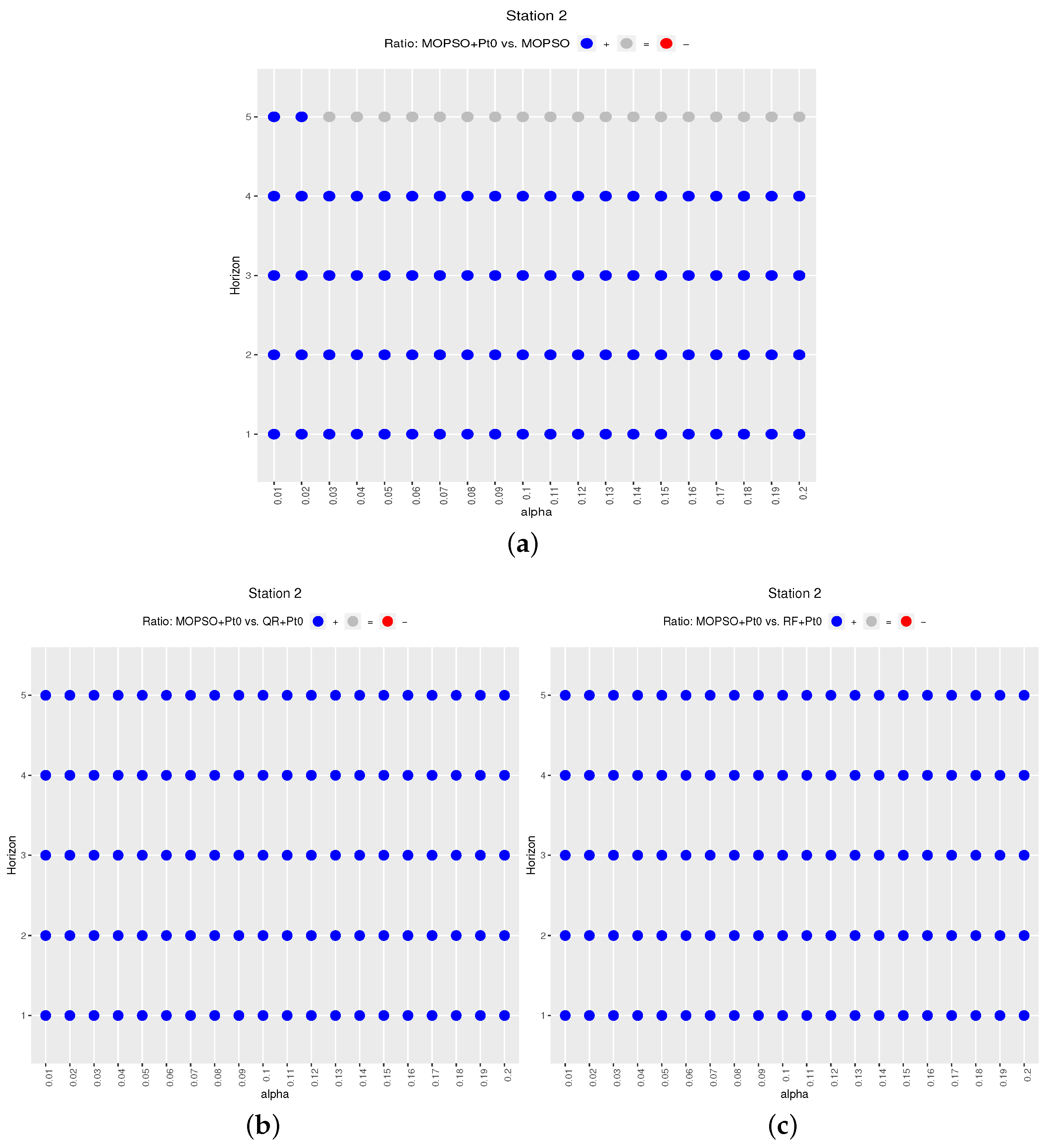
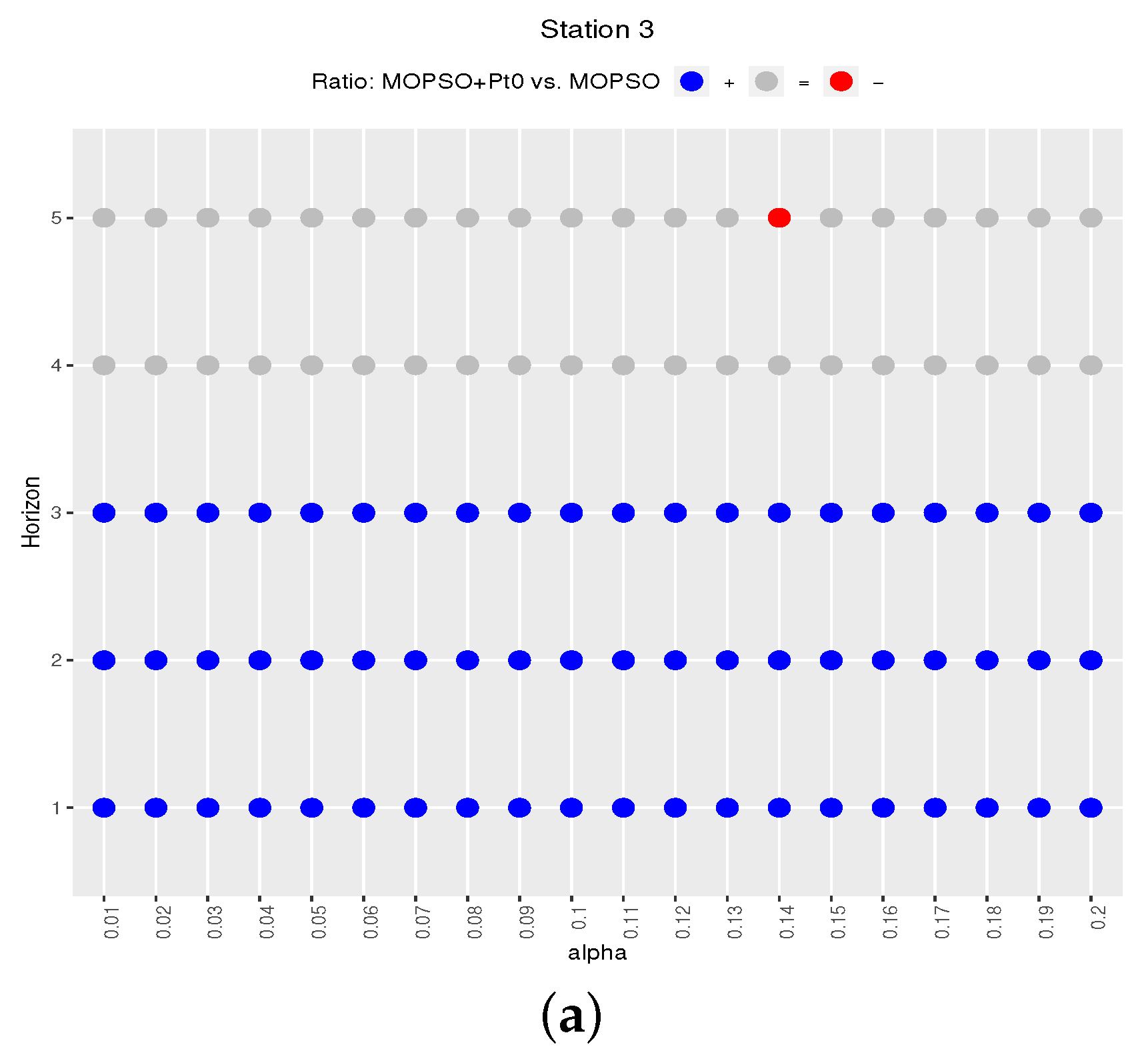
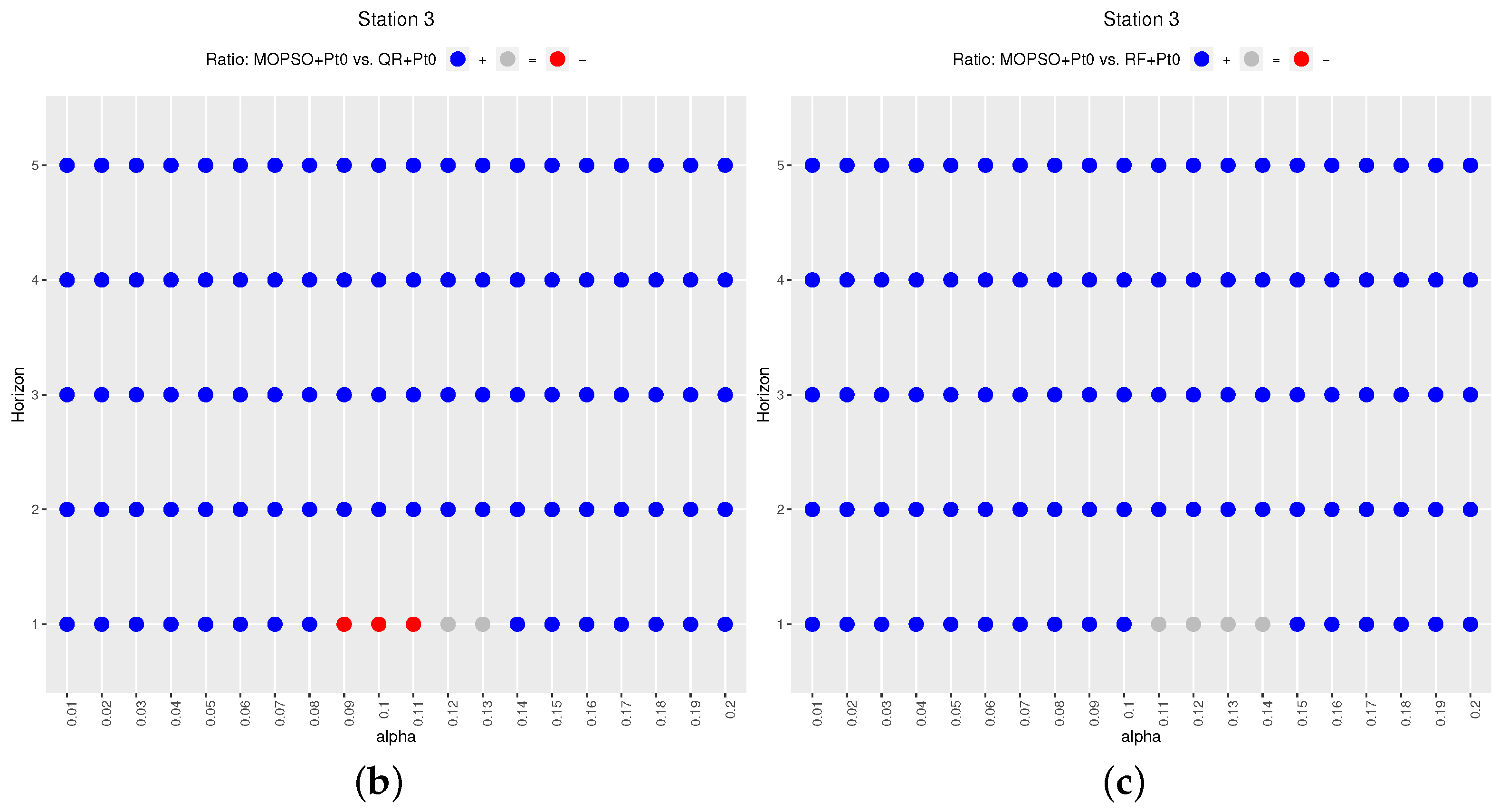
The above figures offer a qualitative view of the results, but, given that and were run 90 times, statistical tests could also be computed. In this work, we used the Wilcoxon test. The results are summarized in Figure 6, for Stations 1–3, repectively. In this case, only tests for the ratio are shown (but follows a similar pattern and can be found in Appendix A. Part (a) (top) of Figure 6 compares and . A blue point is used when the ’s ratio is significantly larger than , and red for the other way around. Color grey signals that and are not statistically different. lThe lower plots (b) and (c) of Figure 6 perform the same comparison, but for versus and for versus . Results for Station 1 (see Figure 6a) show that, indeed, for the first two horizons, ’s ratios are better than ’s (blue points for all s). However, beyond the second hour, is not necessarily significantly better (and, in very few cases, it is significantly worse: red points). The comparisons between and and and offer more systematic results: they are almost all blue points, which means that is basically significantly better than and better than . The second station shows even cleaner results: Figure 7a displays blue points for the first four hours, and mostly grey for the fifth horizon. Again, the blue-filled plot of Figure 7b means that is significantly better than and in all cases. In summary, for Station 2, has a beneficial effect on for even longer horizon spans (up to the fourth hour). Finally, Figure 8 plots results for Station 3. In this case, the top plot shows blue points up to the third hour, all grey for the fourth horizon, but mostly red for the fifth one. With respect to vs. (Figure 8b), it is again mostly blue points, but the anomalies mentioned in the qualitative results pop up again here (red points), for the first horizon and 0.09, 0.1, and 0.11. In this figure it is also observed than the observed similarity of and previously observed for Station 3 and for the first horizon manifests as differences not statistically significant (grey points).
In summary, is significantly better than for the short horizons for all values. For long horizons, is not significantly worse than except for some values (mostly in Station 1). is significantly better than and for all horizons, except for a few values for the first horizon in Station 3.
6. Conclusions
The LUBE approach is an interesting alternative for estimating PIs in the context of probabilistic forecasting because it is able to estimate directly the lower and upper bounds of PIs. LUBE can be optimized by , a multi-objective evolutionary technique, so that neural networks can be trained to simultaneously optimize the two conflicting properties of PIs: coverage and width. The result of this optimization is a Pareto front, from which solutions can be extracted according to the desired coverage value. In this study, this approach was used to address two issues to obtain PIs for solar power forecasting. The first one was to estimate PIs for five intra-day forecasting horizons from 1 to 5 h. The second, and more important one, was to study the influence of using measured solar power at time on the quality of PIs. Previous work has shown that this is useful for improving point forecasting, but we studied this issue in the context of probabilistic forecasting.
The approach was applied to data from three solar stations in Australia and experiments were carried out using two main configurations: (1) using meteorological forecasts variables as inputs to the methods; and (2) using additionally the measured solar output power as input. To analyze how far the influence of measured output reaches, hourly forecasts horizons from 1 to 5 h were used. The quality of prediction intervals was estimated using the coverage/width ratio and the width of the intervals. High values for ratio mean that intervals have a good trade-off between coverage and width. This study was done for several desired coverage values (or ) from 0.01 to 0.20.
The results show that the ratio is improved by using the measured additional information for the two first horizons on the three locations studied and all the desired coverage values. However, although for one of the station this beneficial influence reaches up to the fourth horizon, in none of the stations the ratio is improved for the farthest horizon tested (5 h). The same trend can be observed for interval width. Experiments were replicated 90 times for different random seeds and statistical significance tests were performed, which show that the mentioned results are statistically significant. Thus, it can be concluded that using measured solar power reduces the uncertainty of the intervals for short forecasting horizons.
The approach was compared with and as baseline methods. Both were tested in the same conditions as , with and without the measured power at time . For all approaches, the use of measured power helped to obtain better PIs, especially in the first horizons. The comparison also shows that is significantly better in all cases except a few values in one of the stations.
Author Contributions
All authors participated in all tasks related to this article (conceptualization, software, validation, data curation, writing original draft and review/editing).
Funding
This work was funded by the Spanish Ministry of Science under contract ENE2014-56126-C2-2-R (AOPRIN-SOL project).
Conflicts of Interest
The authors declare no conflict of interest.
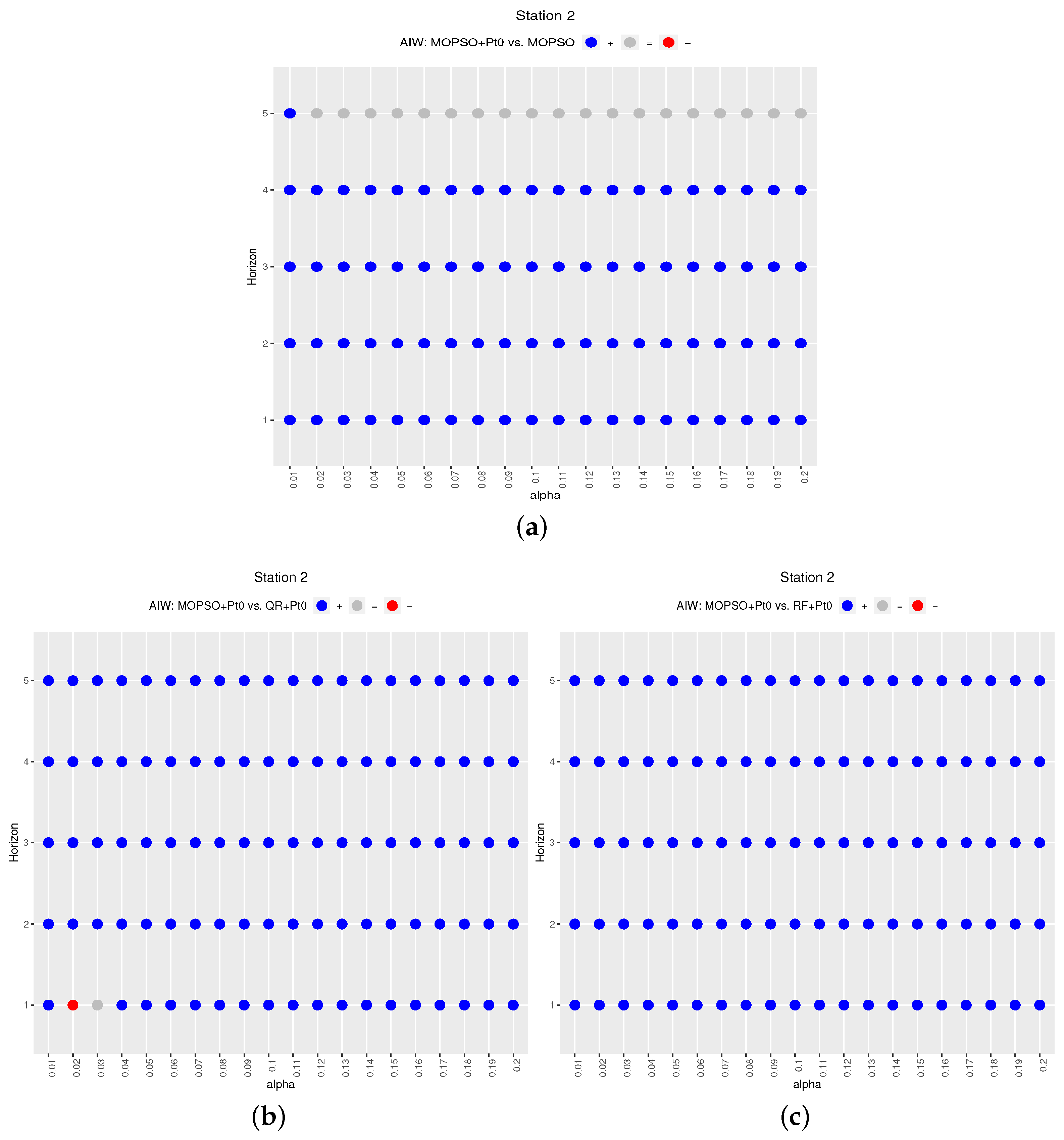
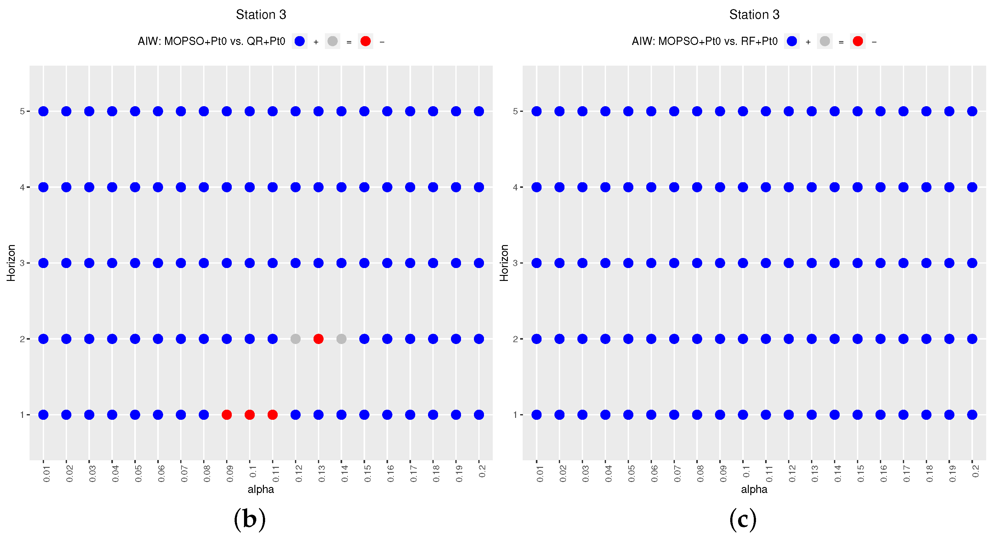
Appendix A
This appendix displays the statistical results for .
Figure A1.
Station 1. Statistical tests for wideness: (a) vs. ; (b) vs. ; and (c) vs. .

Figure A2.
Station 2. Statistical tests for wideness: (a) vs. ; (b) vs. ; and (c) vs. .

Figure A3.
Station 3. Statistical tests for wideness: (a) vs. ; (b) vs. ; and (c) vs. .


References
- Raza, M.Q.; Nadarajah, M.; Ekanayake, C. On recent advances in PV output power forecast. Sol. Energy 2016, 136, 125–144. [Google Scholar] [CrossRef]
- Pinson, P.; Chevallier, C.; Kariniotakis, G.N. Trading wind generation from short-term probabilistic forecasts of wind power. IEEE Trans. Power Syst. 2007, 22, 1148–1156. [Google Scholar] [CrossRef] [Green Version]
- Matos, M.A.; Bessa, R.J. Setting the operating reserve using probabilistic wind power forecasts. IEEE Trans. Power Syst. 2010, 26, 594–603. [Google Scholar] [CrossRef]
- Van der Meer, D.W.; Widén, J.; Munkhammar, J. Review on probabilistic forecasting of photovoltaic power production and electricity consumption. Renew. Sustain. Energy Rev. 2018, 81, 1484–1512. [Google Scholar] [CrossRef]
- Bessa, R.; Möhrlen, C.; Fundel, V.; Siefert, M.; Browell, J.; Haglund El Gaidi, S.; Hodge, B.M.; Cali, U.; Kariniotakis, G. Towards improved understanding of the applicability of uncertainty forecasts in the electric power industry. Energies 2017, 10, 1402. [Google Scholar] [CrossRef]
- Dobschinski, J.; Bessa, R.; Du, P.; Geisler, K.; Haupt, S.E.; Lange, M.; Möhrlen, C.; Nakafuji, D.; de la Torre Rodriguez, M. Uncertainty forecasting in a nutshell: Prediction models designed to prevent significant errors. IEEE Power Energy Mag. 2017, 15, 40–49. [Google Scholar] [CrossRef] [Green Version]
- Koenker, R.; Hallock, K.F. Quantile regression. J. Econ. Perspect. 2001, 15, 143–156. [Google Scholar] [CrossRef]
- Cannon, A.J. Quantile regression neural networks: Implementation in R and application to precipitation downscaling. Comput. Geosci. 2011, 37, 1277–1284. [Google Scholar] [CrossRef]
- Friedman, J.H. Greedy Function Approximation: A Gradient Boosting Machine. Ann. Stat. 2000, 29, 1189–1232. [Google Scholar] [CrossRef]
- Friedman, J.H. Stochastic gradient boosting. Comput. Stat. Data Anal. 2002, 38, 367–378. [Google Scholar] [CrossRef]
- Meinshausen, N. Quantile regression forests. J. Mach. Learn. Res. 2006, 7, 983–999. [Google Scholar]
- Delle Monache, L.; Eckel, F.A.; Rife, D.L.; Nagarajan, B.; Searight, K. Probabilistic weather prediction with an analog ensemble. Mon. Weather Rev. 2013, 141, 3498–3516. [Google Scholar] [CrossRef] [Green Version]
- Cervone, G.; Haupt, S.E. Probabilistic Forecasting of solar energy generation using numerical modeling and remote sensing. In Proceedings of the AGU Fall Meeting Abstracts, San Francisco, CA, USA, 12–16 December 2018. [Google Scholar]
- Clemente-Harding, L.; Young, G.; Cervone, G.; Delle Monache, L.; Haupt, S.E. Toward a Search Space Extension for the Analog Ensemble technique to Improve Probabilistic Predictions. In Proceedings of the AGU Fall Meeting Abstracts, San Francisco, CA, USA, 12–16 December 2018. [Google Scholar]
- Pinson, P.; Nielsen, H.A.; Møller, J.K.; Madsen, H.; Kariniotakis, G.N. Non-parametric probabilistic forecasts of wind power: Required properties and evaluation. Wind Energy 2007, 10, 497–516. [Google Scholar] [CrossRef]
- Khosravi, A.; Nahavandi, S.; Creighton, D.; Atiya, A.F. Lower upper bound estimation method for construction of neural network-based prediction intervals. IEEE Trans. Neural Netw. 2011, 22, 337–346. [Google Scholar] [CrossRef]
- Wan, C.; Xu, Z.; Pinson, P. Direct interval forecasting of wind power. Power Syst. IEEE Trans. 2013, 28, 4877–4878. [Google Scholar] [CrossRef]
- Khosravi, A.; Nahavandi, S. Combined nonparametric prediction intervals for wind power generation. Sustain. Energy IEEE Trans. 2013, 4, 849–856. [Google Scholar] [CrossRef]
- Kirkpatrick, S.; Gelatt, C.D.; Vecchi, M.P. Optimization by simulated annealing. Science 1983, 220, 671–680. [Google Scholar] [CrossRef]
- Eberhart, R.C.; Shi, Y.; Kennedy, J. Swarm Intelligence; Elsevier: Amsterdam, The Netherlands, 2001. [Google Scholar]
- Galván, I.M.; Valls, J.M.; Cervantes, A.; Aler, R. Multi-objective evolutionary optimization of prediction intervals for solar energy forecasting with neural networks. Inf. Sci. 2017, 418, 363–382. [Google Scholar] [CrossRef]
- McGovern, A.; Gagne, D.J.; Basara, J.; Hamill, T.M.; Margolin, D. Solar energy prediction: An international contest to initiate interdisciplinary research on compelling meteorological problems. Bull. Am. Meteorol. Soc. 2015, 96, 1388–1395. [Google Scholar] [CrossRef]
- Aguiar, L.M.; Pereira, B.; Lauret, P.; Díaz, F.; David, M. Combining solar irradiance measurements, satellite-derived data and a numerical weather prediction model to improve intra-day solar forecasting. Renew. Energy 2016, 97, 599–610. [Google Scholar] [CrossRef] [Green Version]
- Wolff, B.; Kühnert, J.; Lorenz, E.; Kramer, O.; Heinemann, D. Comparing support vector regression for PV power forecasting to a physical modeling approach using measurement, numerical weather prediction, and cloud motion data. Sol. Energy 2016, 135, 197–208. [Google Scholar] [CrossRef]
- Martín-Vázquez, R.; Aler, R.; Galván, I. Wind Energy Forecasting at Different Time Horizons with Individual and Global Models. In Proceedings of the IFIP International Conference on Artificial Intelligence Applications and Innovations, lRhodes, Greece, 25–27 May 2018; Springer: New York, NY, USA, 2018; pp. 240–248. [Google Scholar]
- Martín-Vázquez, R.; Huertas-Tato, J.; Aler, R.; Galván, I. Studying the Effect of Measured Solar Power on Evolutionary Multi-objective Prediction Intervals. In Proceedings of the International Conference on Intelligent Data Engineering and Automated Learning, Madrid, Spain, 21–23 November 2018; Springer: New York, NY, USA, 2018; pp. 155–162. [Google Scholar]
- Lauret, P.; David, M.; Pedro, H. Probabilistic solar forecasting using quantile regression models. Energies 2017, 10, 1591. [Google Scholar] [CrossRef]
- Zamo, M.; Mestre, O.; Arbogast, P.; Pannekoucke, O. A benchmark of statistical regression methods for short-term forecasting of photovoltaic electricity production. Part II: Probabilistic forecast of daily production. Sol. Energy 2014, 105, 804–816. [Google Scholar] [CrossRef]
- Abuella, M.; Chowdhury, B. Hourly probabilistic forecasting of solar power. In Proceedings of the IEEE 2017 North American Power Symposium (NAPS), Morgantown, WV, USA, 17–19 September 2017; pp. 1–5. [Google Scholar]
- Hong, T.; Pinson, P.; Fan, S.; Zareipour, H.; Troccoli, A.; Hyndman, R.J. Probabilistic energy forecasting: Global Energy Forecasting Competition 2014 and beyond. Int. J. Forecast. 2016, 32, 896–913. [Google Scholar] [CrossRef] [Green Version]
- Breiman, L. Random forests. Mach. Learn. 2001, 45, 5–32. [Google Scholar] [CrossRef] [Green Version]
Figure 1.
Box plot of solar normalized power, broken down by hour, for: Station 1 (left); Station 2 (middle); and Station 3 (right). The x-axis displays UTC hour.
Figure 1.
Box plot of solar normalized power, broken down by hour, for: Station 1 (left); Station 2 (middle); and Station 3 (right). The x-axis displays UTC hour.

Figure 2.
Station 1: (a) ratio per prediction horizon; and (b) per prediction horizon. values = 0.02 to 0.2.
Figure 2.
Station 1: (a) ratio per prediction horizon; and (b) per prediction horizon. values = 0.02 to 0.2.

Figure 3.
Station 2: (a) ratio per prediction horizon; and (b) per prediction horizon. values = 0.02 to 0.2.
Figure 3.
Station 2: (a) ratio per prediction horizon; and (b) per prediction horizon. values = 0.02 to 0.2.

Figure 4.
Station 3: (a) ratio per prediction horizon; and (b) per prediction horizon. values = 0.02 to 0.2.
Figure 4.
Station 3: (a) ratio per prediction horizon; and (b) per prediction horizon. values = 0.02 to 0.2.

Figure 5.
PIs for the five forecast horizons for four specific days of the year (one day per row): The left column compares (grey) with (yellow) and the right column compares (grey) with (yellow).
Figure 5.
PIs for the five forecast horizons for four specific days of the year (one day per row): The left column compares (grey) with (yellow) and the right column compares (grey) with (yellow).

Figure 6.
Station 1. Statistical tests for ratio: (a) vs. ; (b) vs. ; and (c) vs. .

Figure 7.
Station 2. Statistical tests for ratio: (a) vs. ; (b) vs. ; and (c) vs. .

Figure 8.
Station 3. Statistical tests for ratio: (a) vs. ; (b) vs. ; and (c) vs. .


Table 1.
Best combination of parameters for each prediction horizon.
| Station 1 | ||||
|---|---|---|---|---|
| Horizon | Neurons | Iterations | Neurons | Iterations |
| 1 h | ||||
| 2 h | ||||
| 3 h | ||||
| 4 h | ||||
| 5 h | ||||
| Station 2 | ||||
| Horizon | Neurons | Iterations | Neurons | Iterations |
| 1 h | ||||
| 2 h | ||||
| 3 h | ||||
| 4 h | ||||
| 5 h | ||||
| Station 3 | ||||
| Horizon | Neurons | Iterations | Neurons | Iterations |
| 1 h | ||||
| 2 h | ||||
| 3 h | ||||
| 4 h | ||||
| 5 h | ||||
Table 2.
Means of ratios for all the values, for each prediction horizon and each method (Stations 1–3).
Table 2.
Means of ratios for all the values, for each prediction horizon and each method (Stations 1–3).
| Station 1 | ||||||
|---|---|---|---|---|---|---|
| Horizon | ||||||
| 1 | 2.07 | 2.69 | 1.71 | 2.47 | 1.80 | 2.58 |
| 2 | 2.23 | 2.30 | 1.80 | 1.98 | 1.88 | 1.96 |
| 3 | 2.35 | 2.34 | 1.90 | 1.91 | 1.97 | 1.98 |
| 4 | 2.37 | 2.36 | 1.92 | 1.95 | 2.01 | 2.01 |
| 5 | 2.33 | 2.33 | 2.04 | 2.08 | 2.16 | 2.18 |
| Station 2 | ||||||
| Horizon | ||||||
| 1 | 2.23 | 2.79 | 1.77 | 2.52 | 1.96 | 2.61 |
| 2 | 2.14 | 2.34 | 1.77 | 1.95 | 1.83 | 2.00 |
| 3 | 2.06 | 2.15 | 1.76 | 1.92 | 1.76 | 1.87 |
| 4 | 2.02 | 2.10 | 1.68 | 1.78 | 1.68 | 1.81 |
| 5 | 1.89 | 1.89 | 1.58 | 1.60 | 1.61 | 1.63 |
| Station 3 | ||||||
| Horizon | ||||||
| 1 | 2.37 | 2.89 | 2.02 | 2.77 | 2.09 | 2.84 |
| 2 | 2.30 | 2.41 | 2.02 | 2.20 | 1.97 | 2.14 |
| 3 | 2.15 | 2.20 | 1.96 | 2.01 | 1.90 | 1.95 |
| 4 | 2.13 | 2.14 | 1.92 | 1.95 | 1.85 | 1.89 |
| 5 | 2.11 | 2.09 | 1.90 | 1.91 | 1.86 | 1.87 |
© 2019 by the authors. Licensee MDPI, Basel, Switzerland. This article is an open access article distributed under the terms and conditions of the Creative Commons Attribution (CC BY) license (http://creativecommons.org/licenses/by/4.0/).
Share and Cite
MDPI and ACS Style
Aler, R.; Huertas-Tato, J.; Valls, J.M.; Galván, I.M. Improving Prediction Intervals Using Measured Solar Power with a Multi-Objective Approach. Energies 2019, 12, 4713. https://doi.org/10.3390/en12244713
AMA Style
Aler R, Huertas-Tato J, Valls JM, Galván IM. Improving Prediction Intervals Using Measured Solar Power with a Multi-Objective Approach. Energies. 2019; 12(24):4713. https://doi.org/10.3390/en12244713
Chicago/Turabian StyleAler, Ricardo, Javier Huertas-Tato, José M. Valls, and Inés M. Galván. 2019. "Improving Prediction Intervals Using Measured Solar Power with a Multi-Objective Approach" Energies 12, no. 24: 4713. https://doi.org/10.3390/en12244713
Note that from the first issue of 2016, this journal uses article numbers instead of page numbers. See further details here.