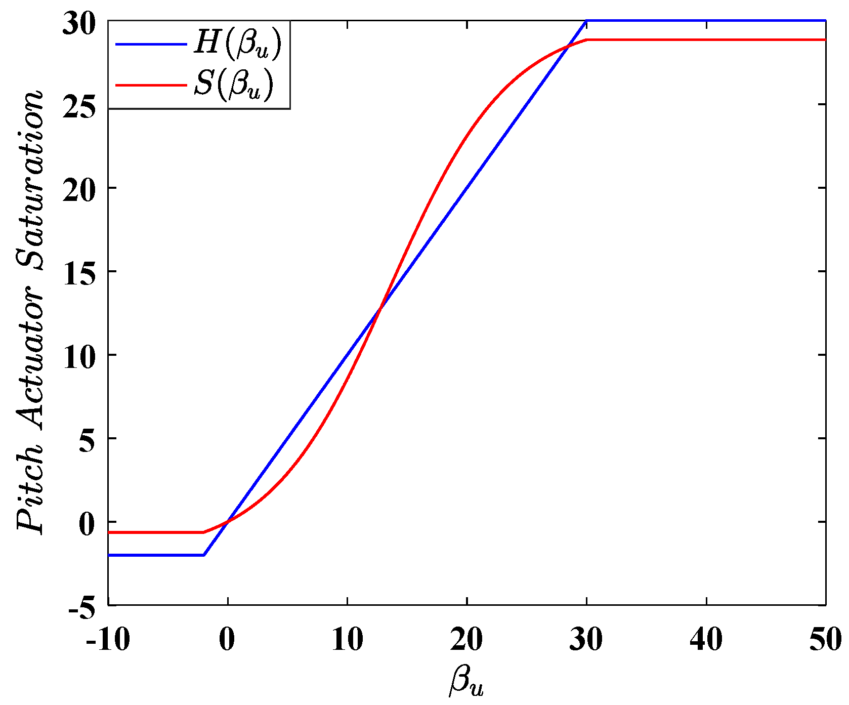
Figure 1.
Pitch actuator saturation, (blue line), and its smooth estimation, (red line).
Figure 1.
Pitch actuator saturation, (blue line), and its smooth estimation, (red line).
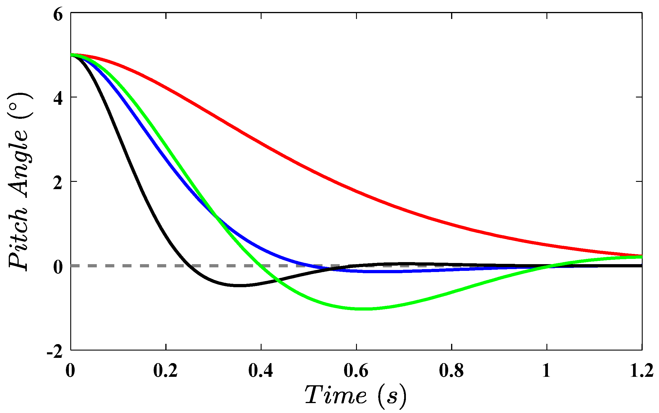
Figure 2.
Pitch actuator response in situations: normal (black line), hydraulic leak (red line), pump wear (blue line), and high air content (green line).
Figure 2.
Pitch actuator response in situations: normal (black line), hydraulic leak (red line), pump wear (blue line), and high air content (green line).
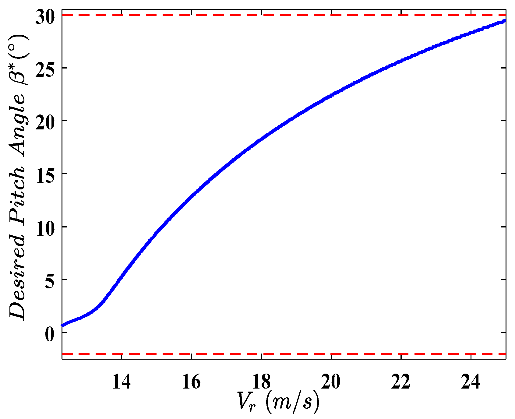
Figure 3.
Diagram of (blue line), and lower and upper pitch angle bounds (red dashed lines).
Figure 3.
Diagram of (blue line), and lower and upper pitch angle bounds (red dashed lines).
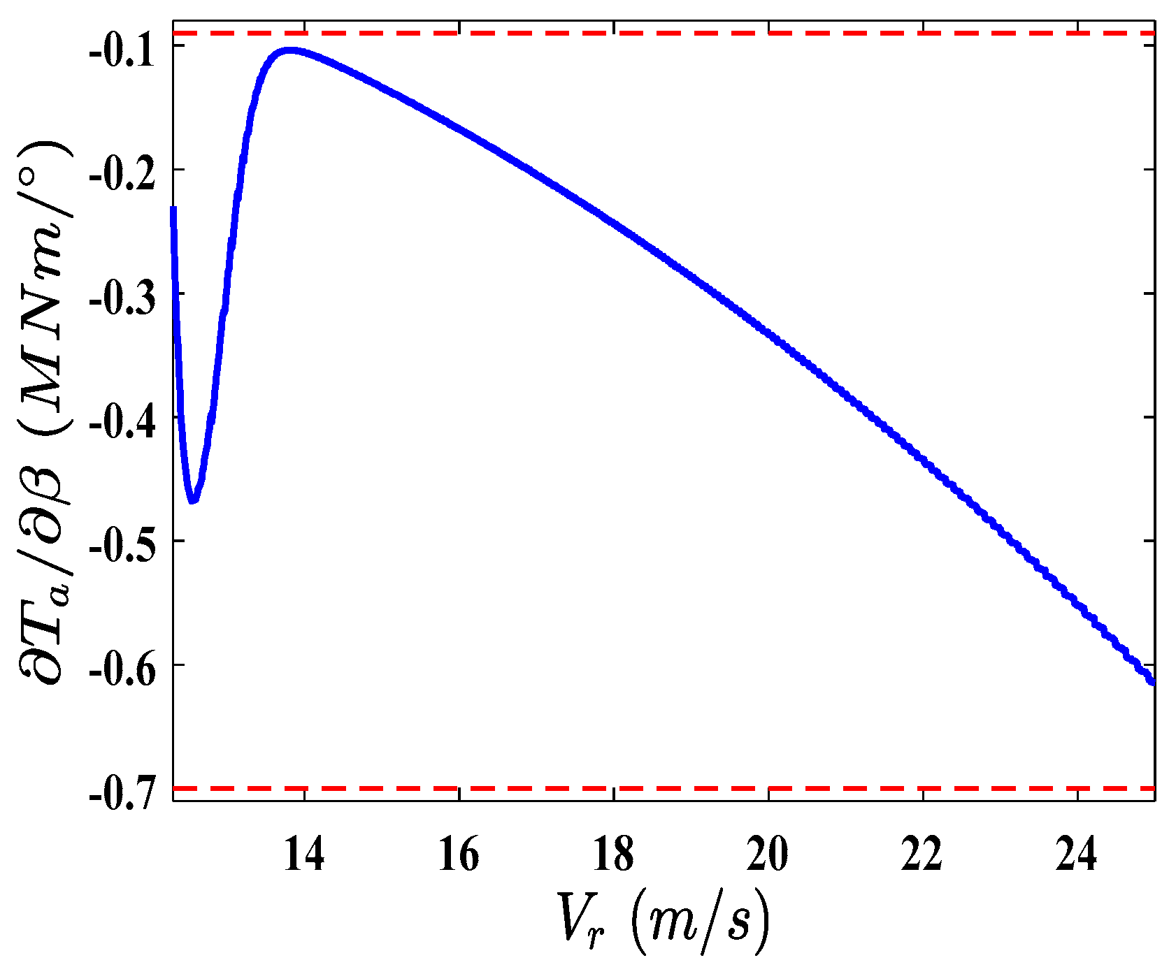
Figure 4.
diagram in full load operation (blue line), and upper and lower bounds (red dashed lines).
Figure 4.
diagram in full load operation (blue line), and upper and lower bounds (red dashed lines).
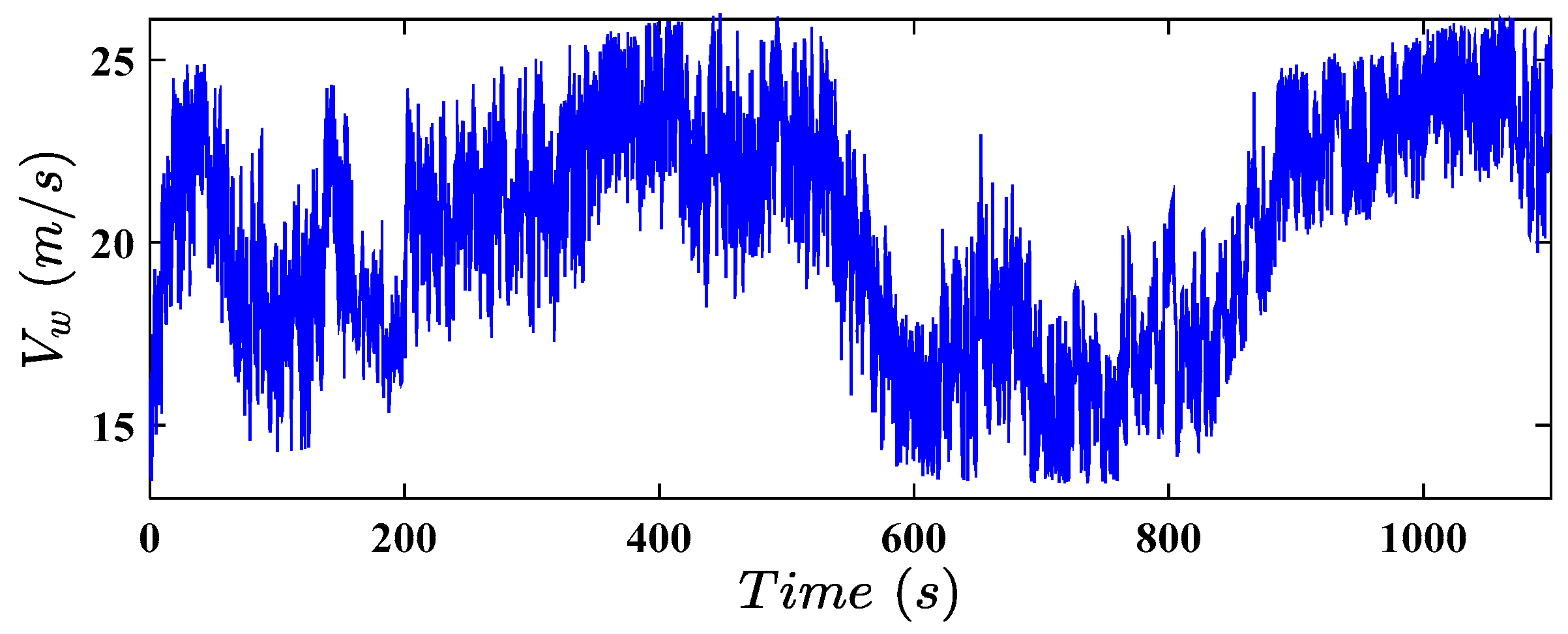
Figure 5.
Free wind speed profile.
Figure 5.
Free wind speed profile.
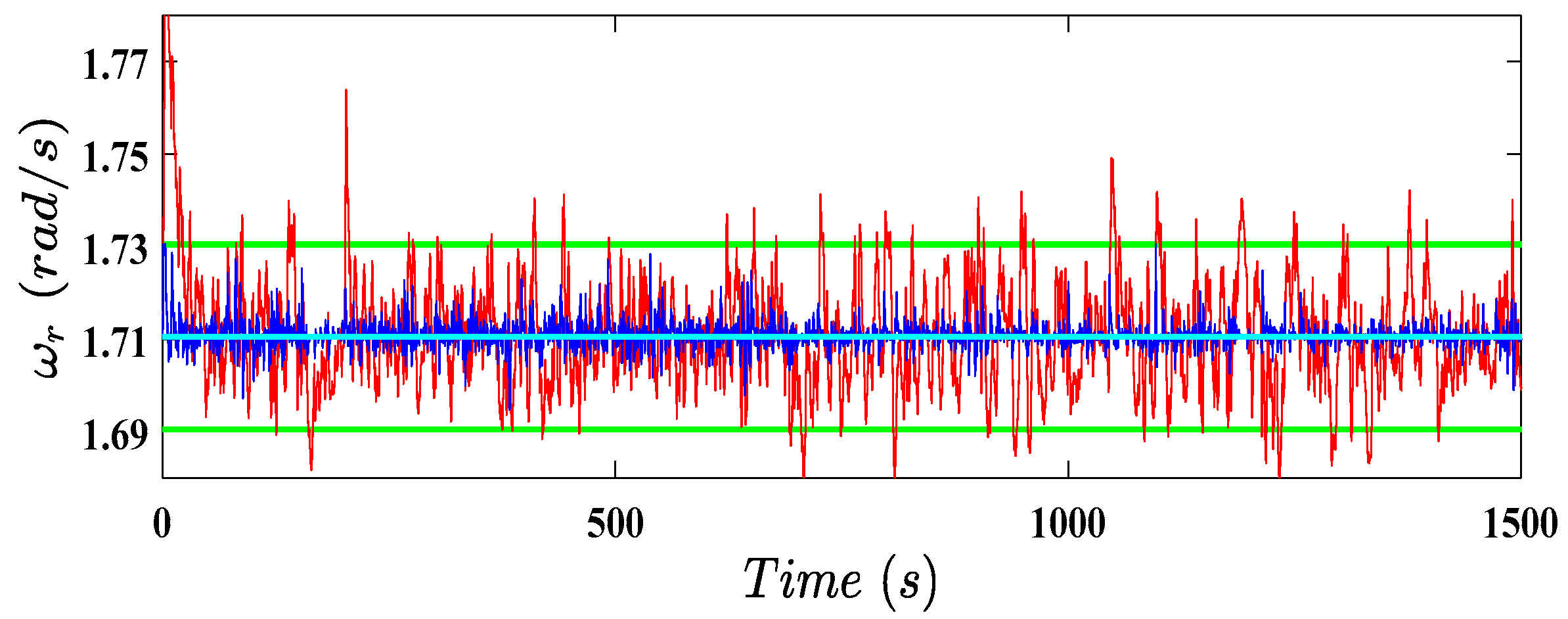
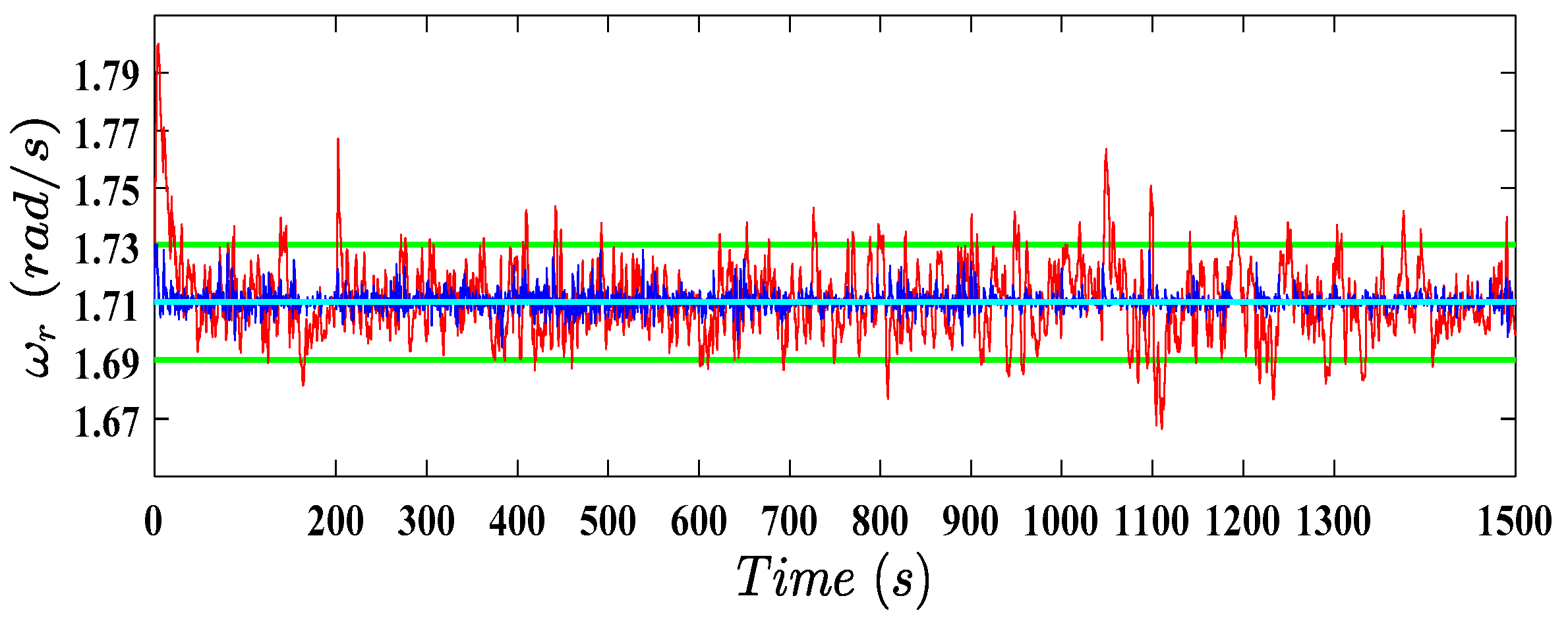
Figure 6.
Rotor speed using the proposed controller (dark blue line), PID controller (red line), nominal rotor speed (light blue line), and constraints (green line), in the fault-free situation.
Figure 6.
Rotor speed using the proposed controller (dark blue line), PID controller (red line), nominal rotor speed (light blue line), and constraints (green line), in the fault-free situation.
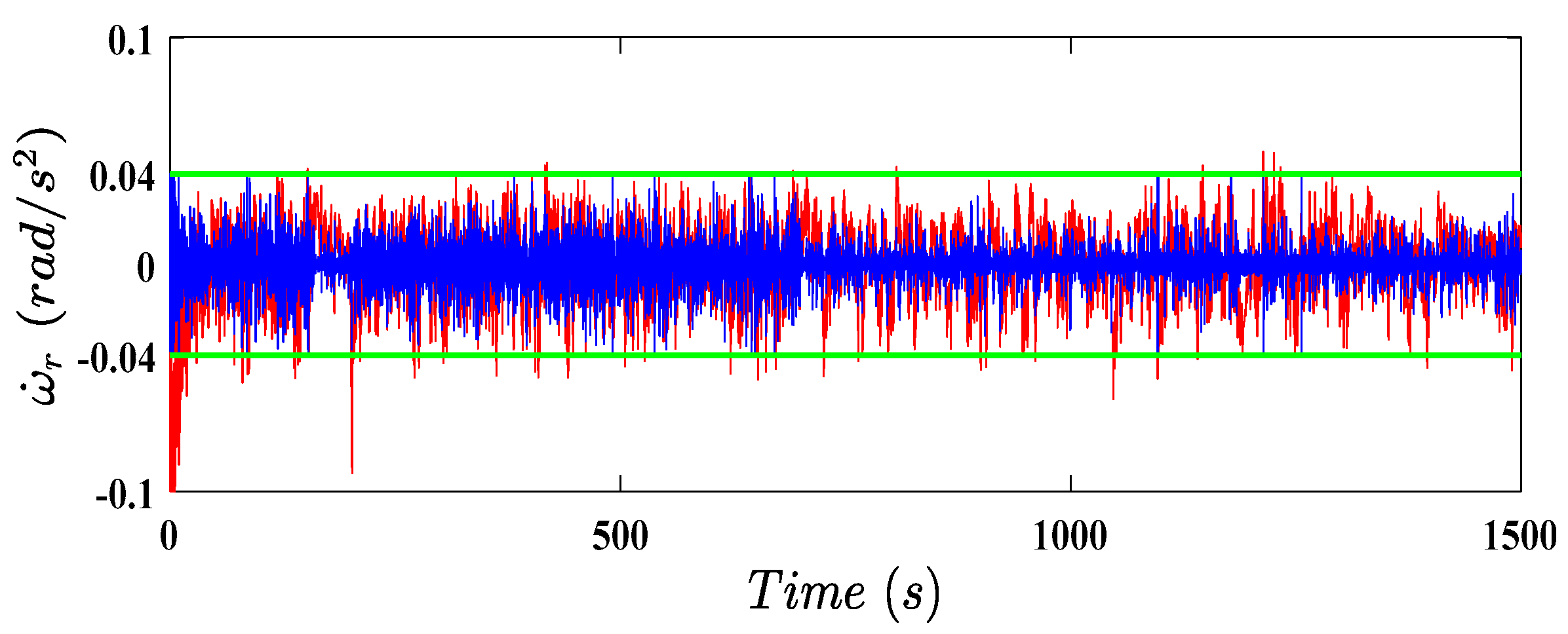
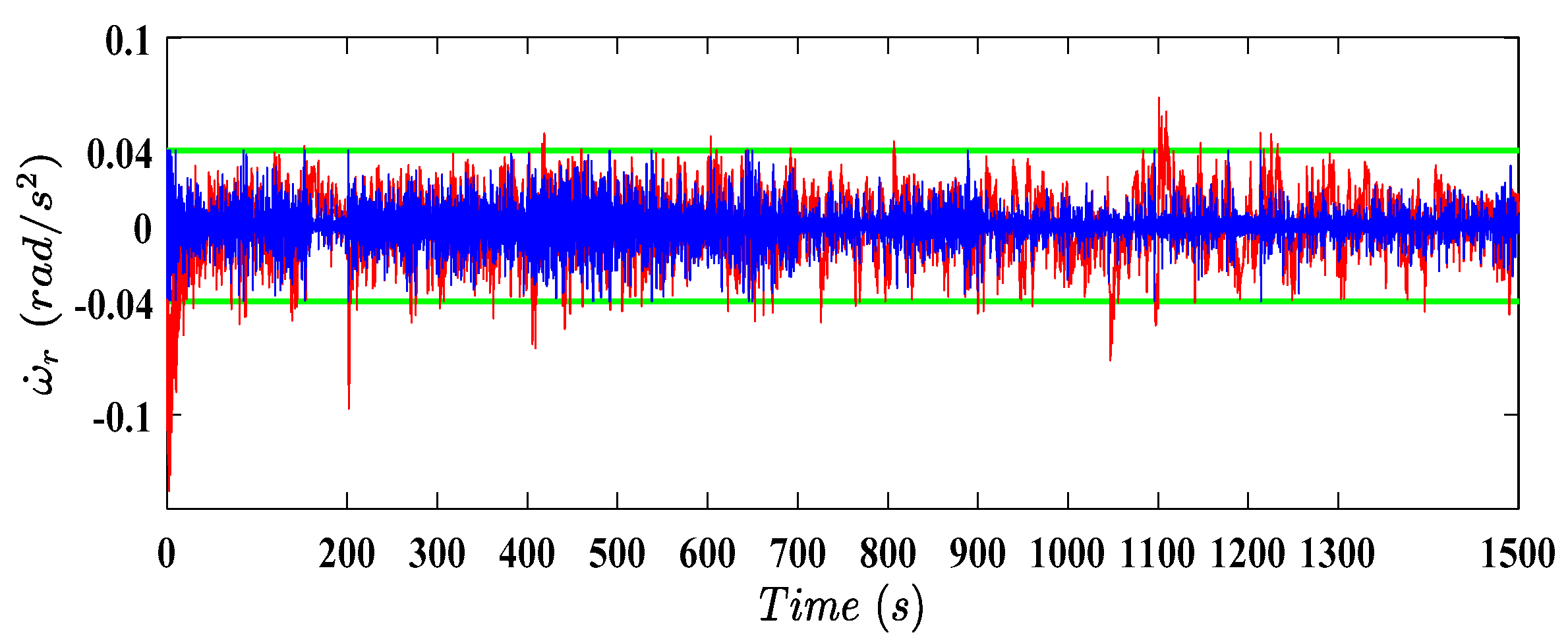
Figure 7.
Rotor acceleration using the proposed controller (dark blue line), PID controller (red line), and constraints (green line), in the fault-free situation.
Figure 7.
Rotor acceleration using the proposed controller (dark blue line), PID controller (red line), and constraints (green line), in the fault-free situation.
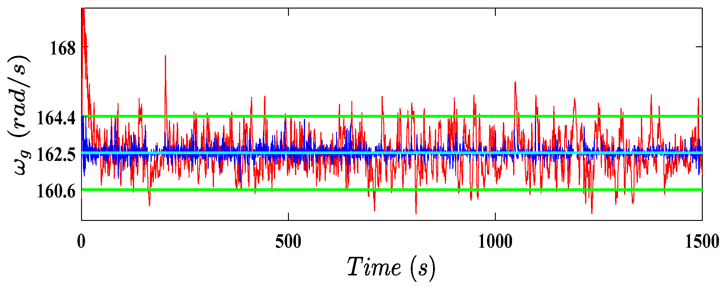
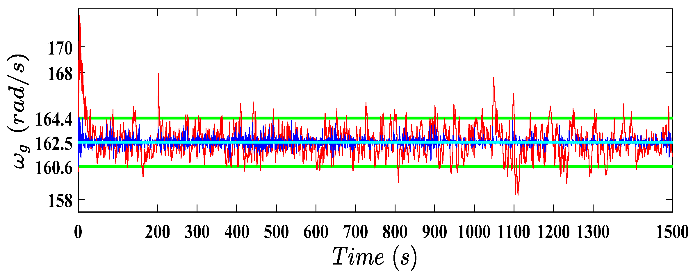
Figure 8.
Generator speed using the proposed controller (dark blue line), PID controller (red line), nominal generator speed (light blue line), and constraints (green line), in the fault-free situation.
Figure 8.
Generator speed using the proposed controller (dark blue line), PID controller (red line), nominal generator speed (light blue line), and constraints (green line), in the fault-free situation.
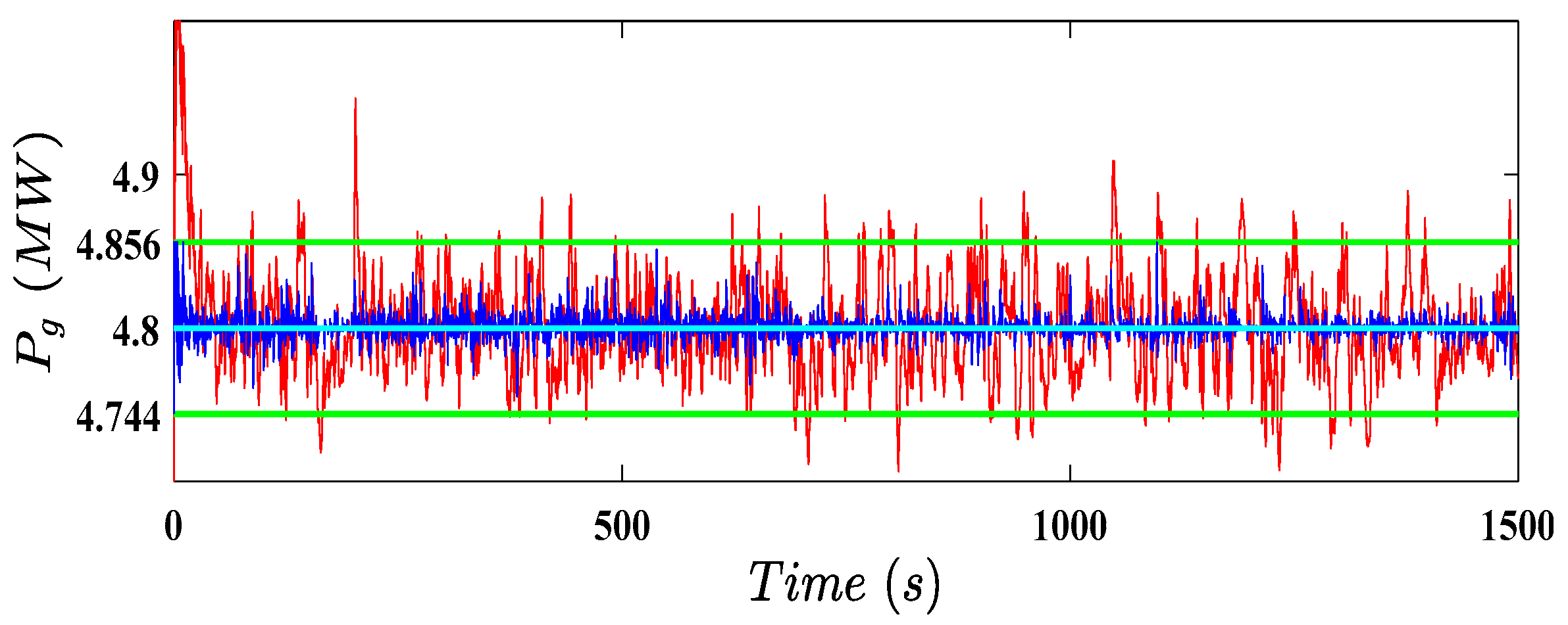
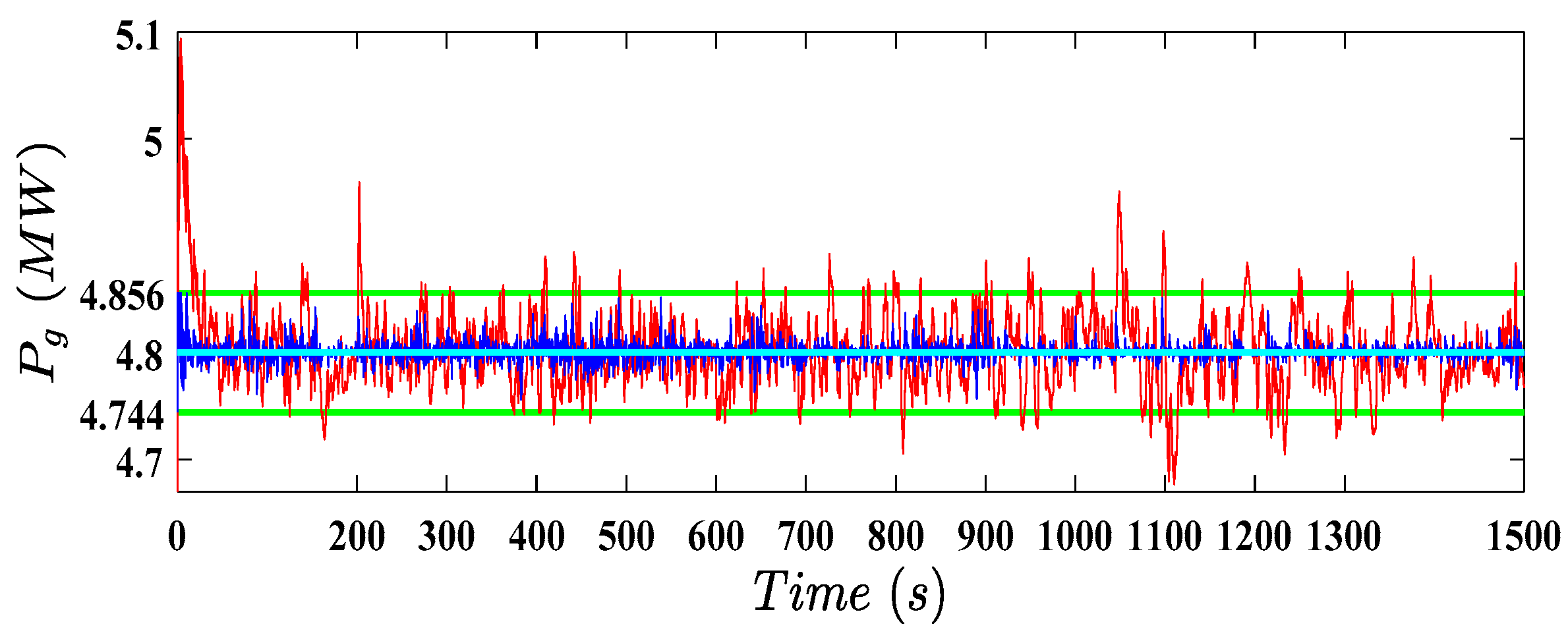
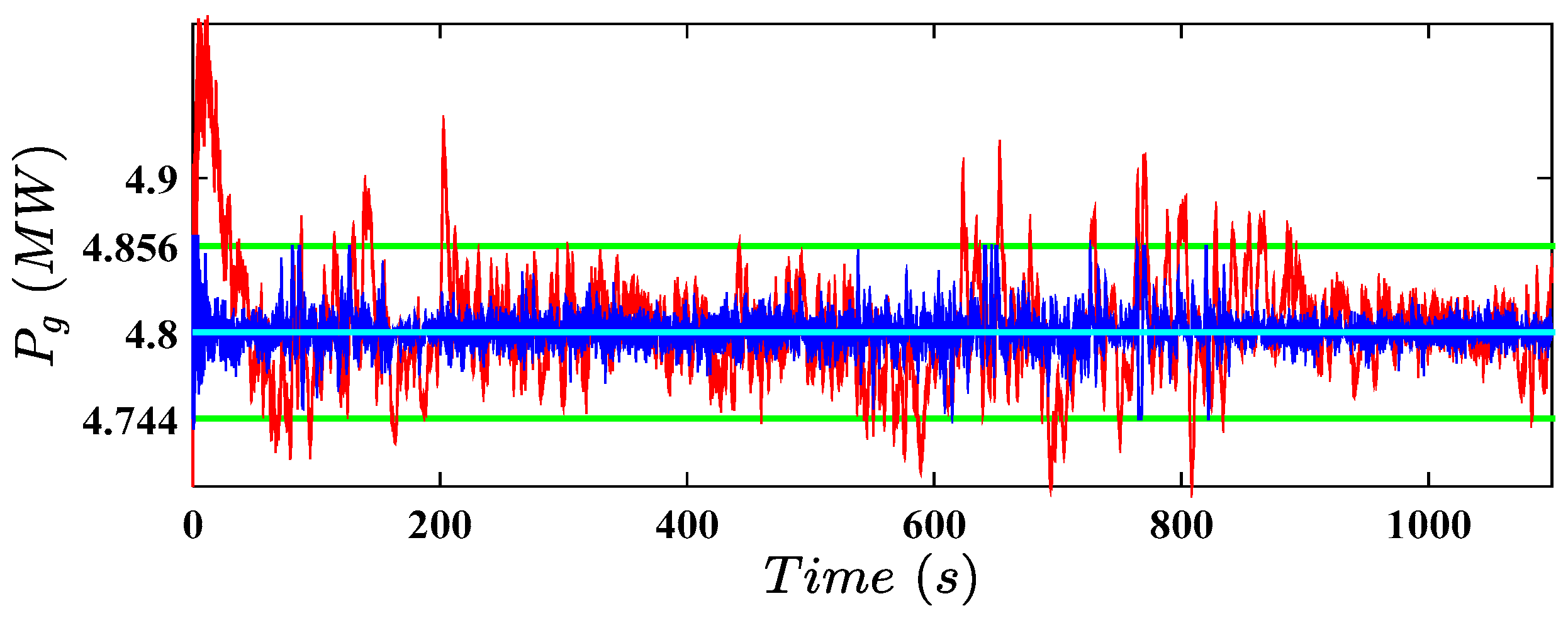
Figure 9.
Generated power using the proposed controller (dark blue line), PID controller (red line), nominal power (light blue line), and constraints (green line), in the fault-free situation.
Figure 9.
Generated power using the proposed controller (dark blue line), PID controller (red line), nominal power (light blue line), and constraints (green line), in the fault-free situation.
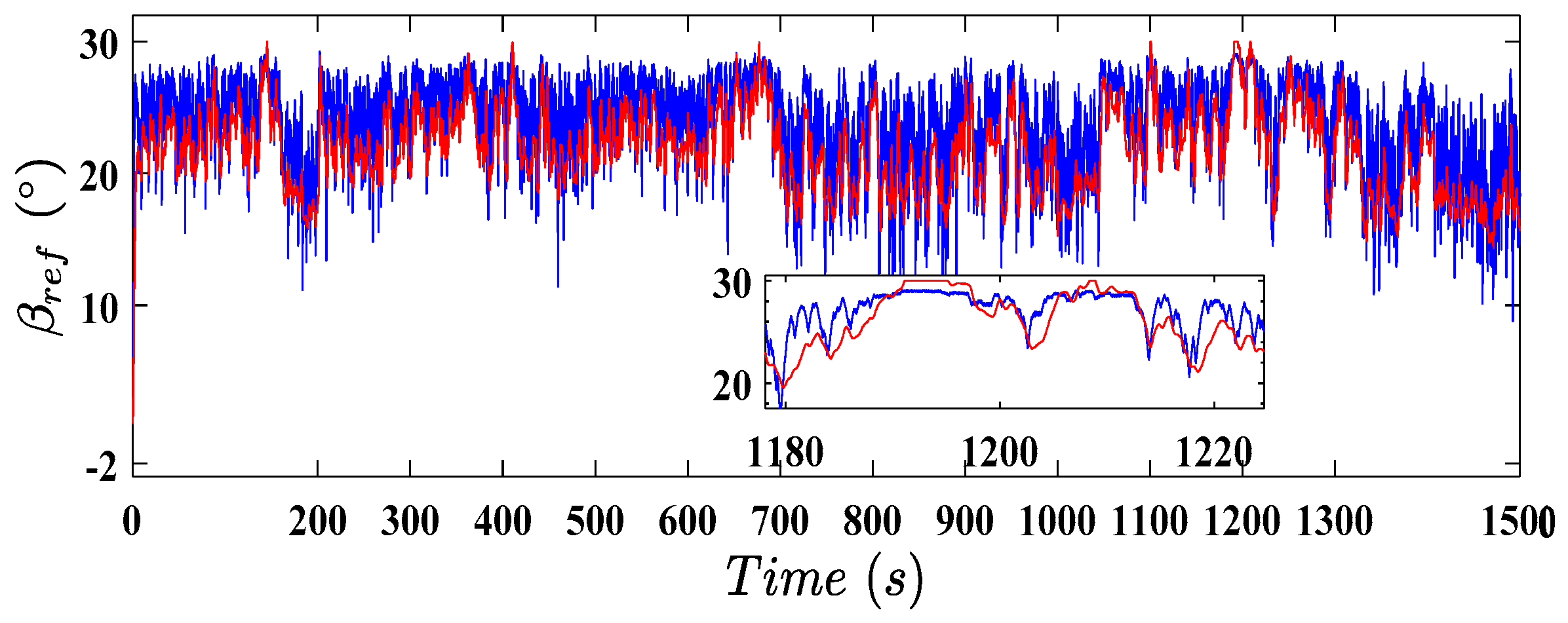
Figure 10.
Reference pitch angle using the proposed controller (dark blue line) and PID controller (red line), in the fault-free situation.
Figure 10.
Reference pitch angle using the proposed controller (dark blue line) and PID controller (red line), in the fault-free situation.
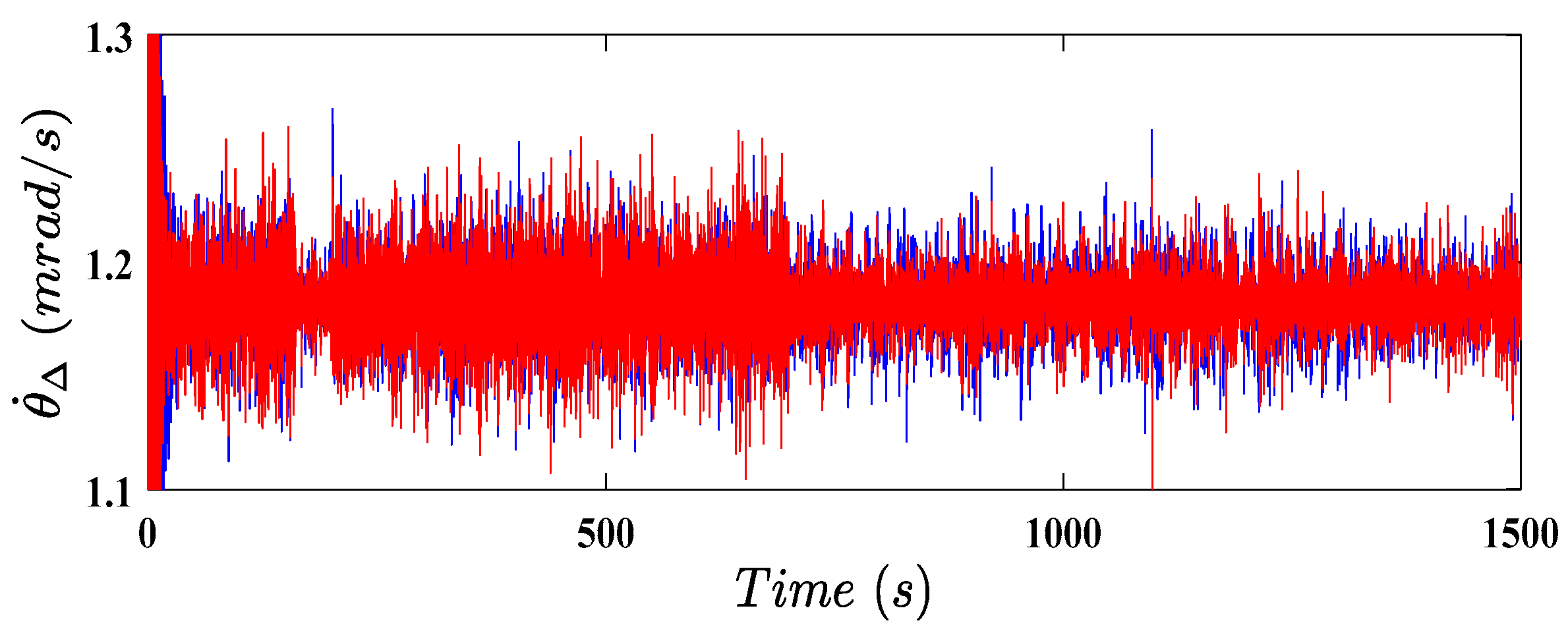
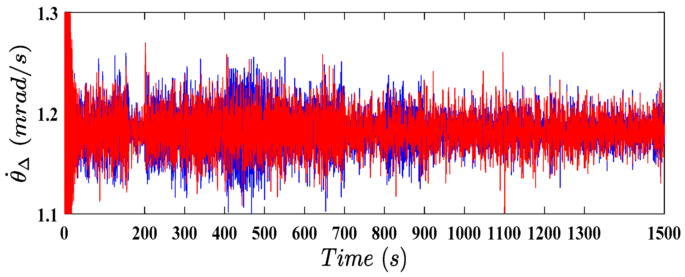
Figure 11.
Induced drive train torsion angle rate using the proposed controller (dark blue line) and PID controller (red line), in the fault-free situation.
Figure 11.
Induced drive train torsion angle rate using the proposed controller (dark blue line) and PID controller (red line), in the fault-free situation.
Figure 12.
Actual aerodynamic torque (red line), estimated one (dark blue line), and nominal one (light blue line).
Figure 12.
Actual aerodynamic torque (red line), estimated one (dark blue line), and nominal one (light blue line).
Figure 13.
Rotor speed using the proposed controller (dark blue line), PID controller (red line), nominal rotor speed (light blue line), and constraints (green line), with the first fault scenario.
Figure 13.
Rotor speed using the proposed controller (dark blue line), PID controller (red line), nominal rotor speed (light blue line), and constraints (green line), with the first fault scenario.
Figure 14.
Rotor acceleration using the proposed controller (dark blue line), PID controller (red line), and constraints (green line), with the first fault scenario.
Figure 14.
Rotor acceleration using the proposed controller (dark blue line), PID controller (red line), and constraints (green line), with the first fault scenario.
Figure 15.
Generator speed using the proposed controller (dark blue line), PID controller (red line), nominal generator speed (light blue line), and constraints (green line), with the first fault scenario.
Figure 15.
Generator speed using the proposed controller (dark blue line), PID controller (red line), nominal generator speed (light blue line), and constraints (green line), with the first fault scenario.
Figure 16.
Generated power using the proposed controller (dark blue line), PID controller (red line), nominal power (light blue line), and constraints (green line), with the first fault scenario.
Figure 16.
Generated power using the proposed controller (dark blue line), PID controller (red line), nominal power (light blue line), and constraints (green line), with the first fault scenario.
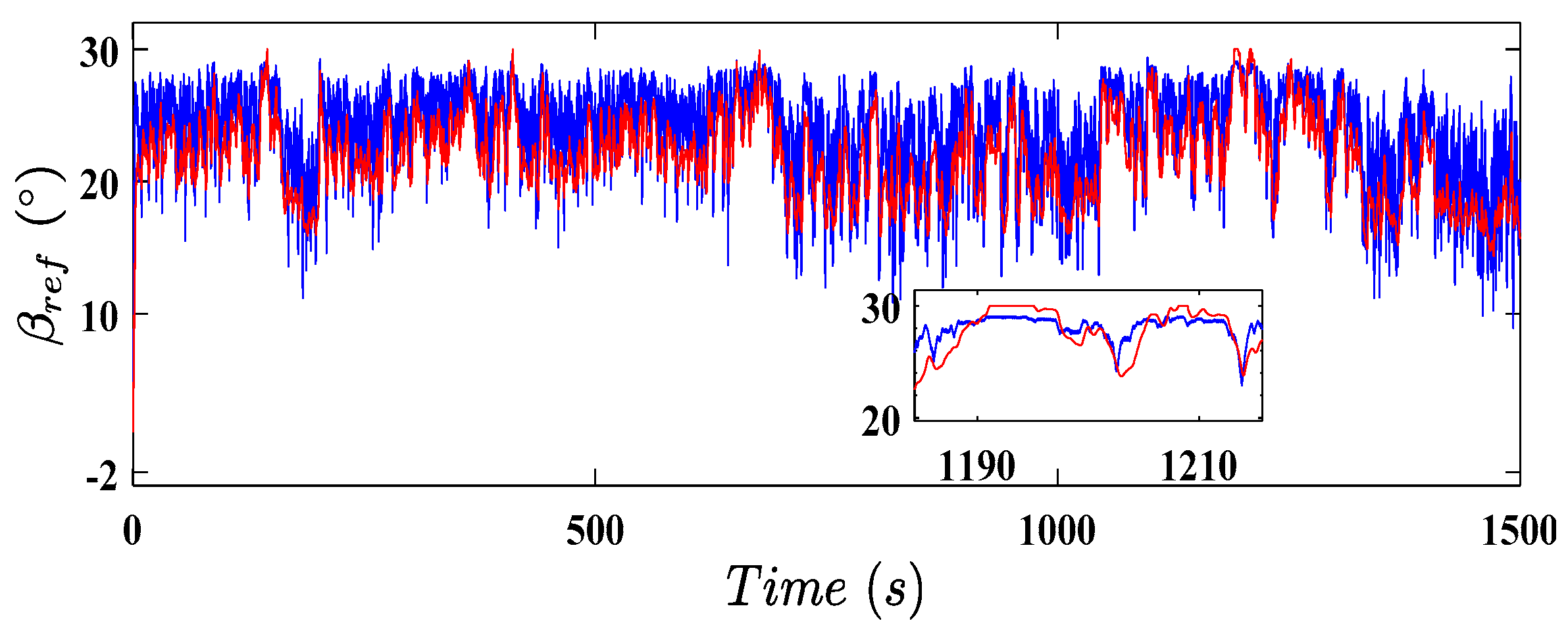
Figure 17.
Reference pitch angle using the proposed controller (dark blue line) and PID controller (red line), with the first fault scenario.
Figure 17.
Reference pitch angle using the proposed controller (dark blue line) and PID controller (red line), with the first fault scenario.
Figure 18.
Induced drive train torsion angle rate using the proposed controller (dark blue line) and PID controller (red line), with the first fault scenario.
Figure 18.
Induced drive train torsion angle rate using the proposed controller (dark blue line) and PID controller (red line), with the first fault scenario.
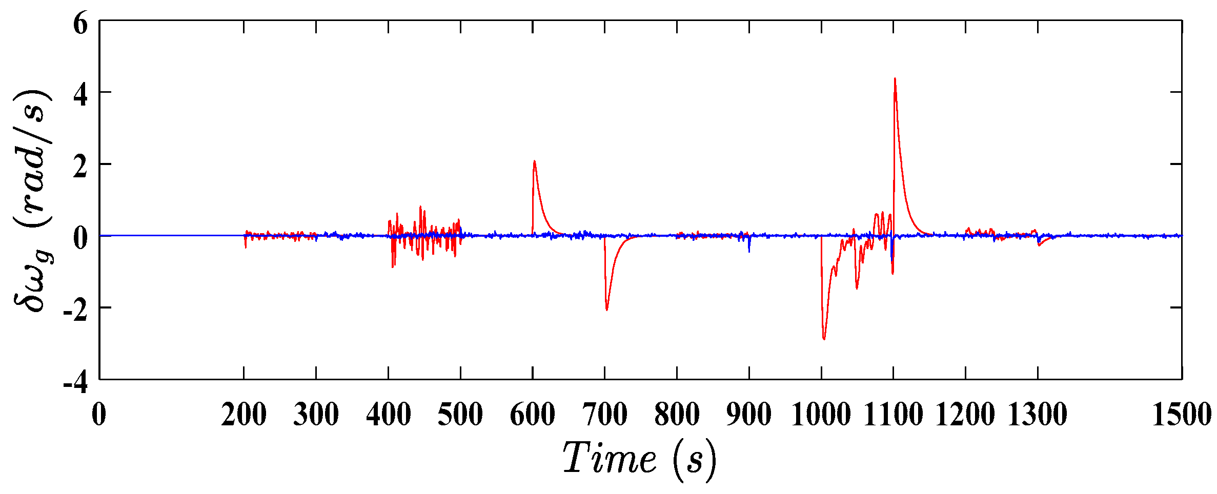
Figure 19.
using the proposed controller (dark blue line) and PID controller (red line), with the first fault scenario.
Figure 19.
using the proposed controller (dark blue line) and PID controller (red line), with the first fault scenario.
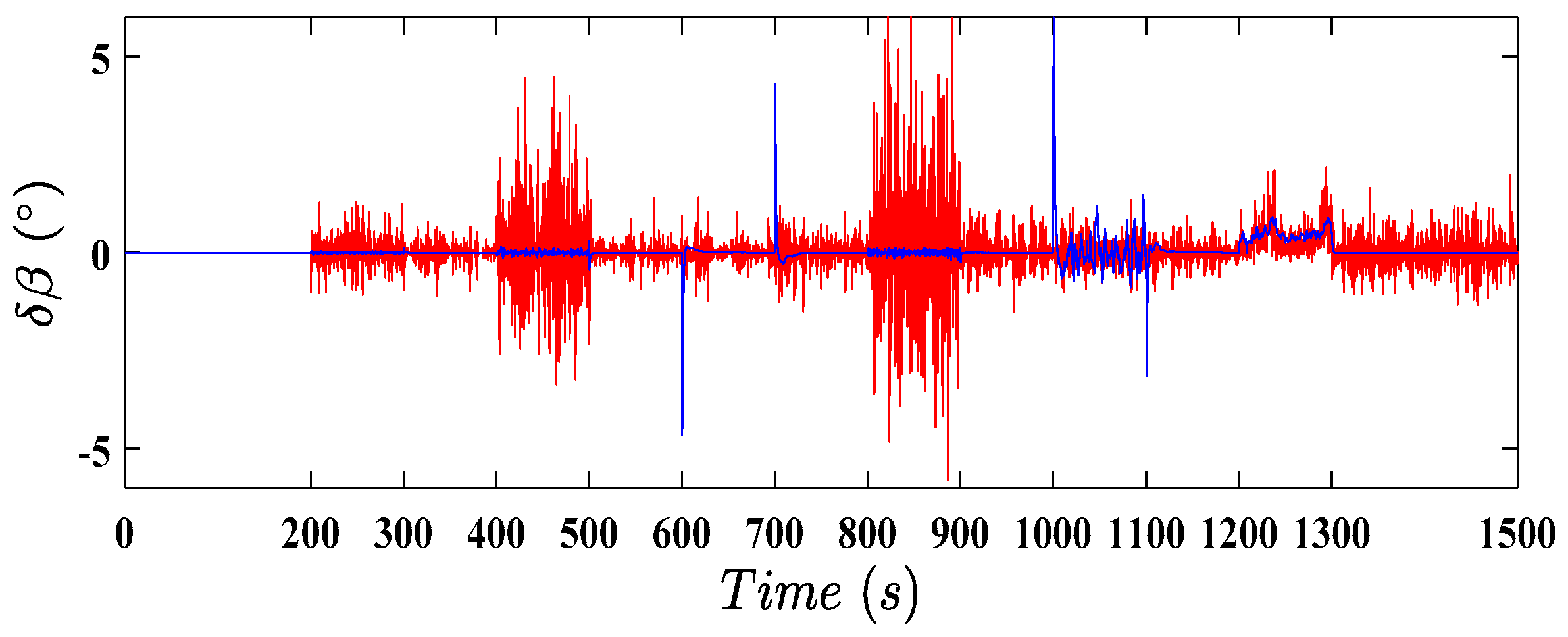
Figure 20.
using the proposed controller (dark blue line) and PID controller (red line), with the first fault scenario.
Figure 20.
using the proposed controller (dark blue line) and PID controller (red line), with the first fault scenario.
Figure 21.
using the proposed controller (dark blue line) and PID controller (red line), with the first fault scenario.
Figure 21.
using the proposed controller (dark blue line) and PID controller (red line), with the first fault scenario.
Figure 22.
using the proposed controller (dark blue line) and PID controller (red line), with the first fault scenario.
Figure 22.
using the proposed controller (dark blue line) and PID controller (red line), with the first fault scenario.
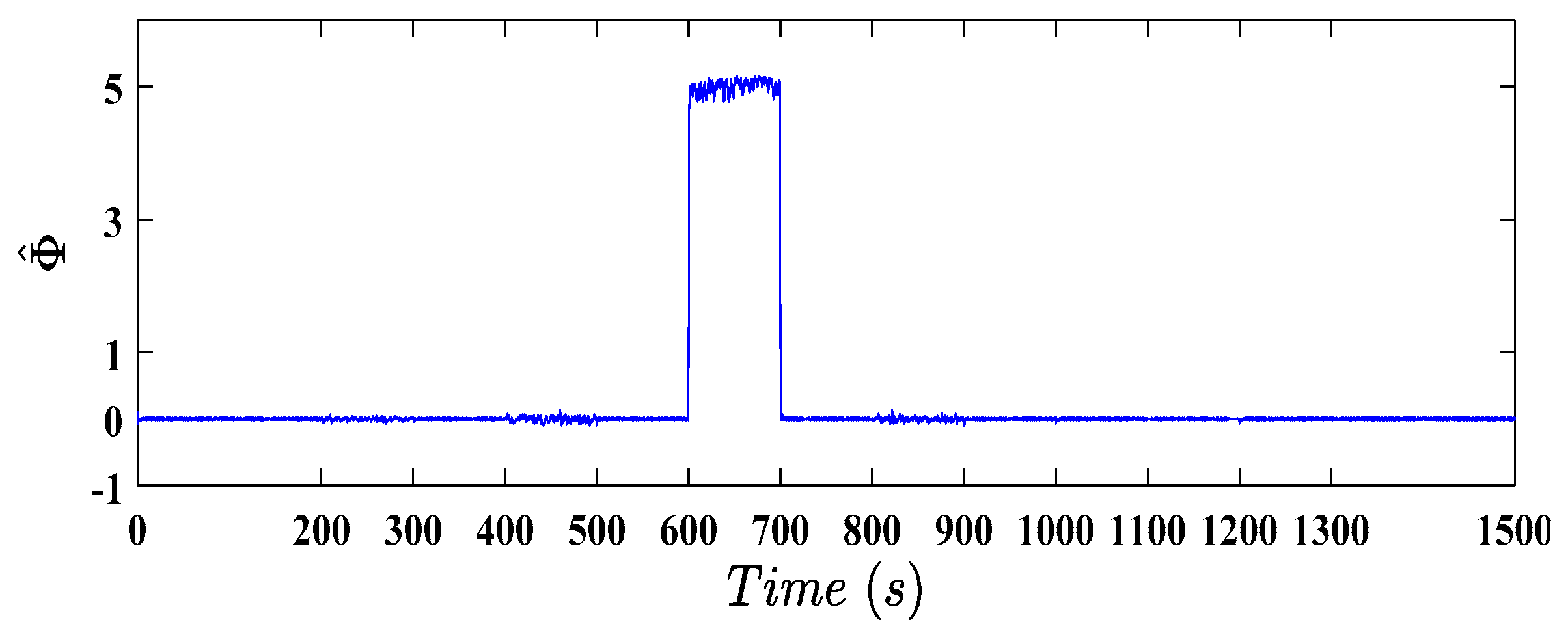
Figure 23.
Estimated fault.
Figure 23.
Estimated fault.
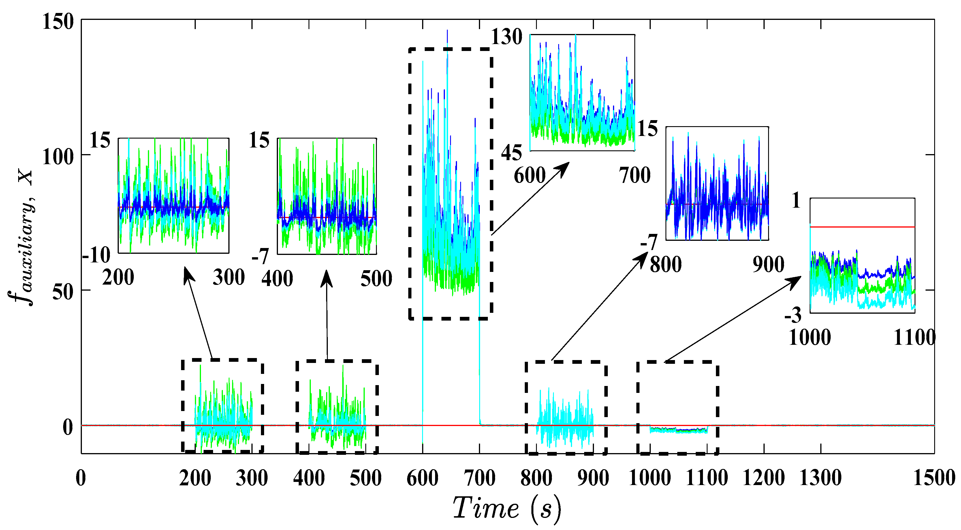
Figure 24.
Auxiliary signal in the case of fault-free (red line), pump wear (dark blue line), high air content (green line), and hydraulic leak (light blue line).
Figure 24.
Auxiliary signal in the case of fault-free (red line), pump wear (dark blue line), high air content (green line), and hydraulic leak (light blue line).
Figure 25.
Estimated pitch actuator bias.
Figure 25.
Estimated pitch actuator bias.
Figure 26.
Second free wind speed profile.
Figure 26.
Second free wind speed profile.
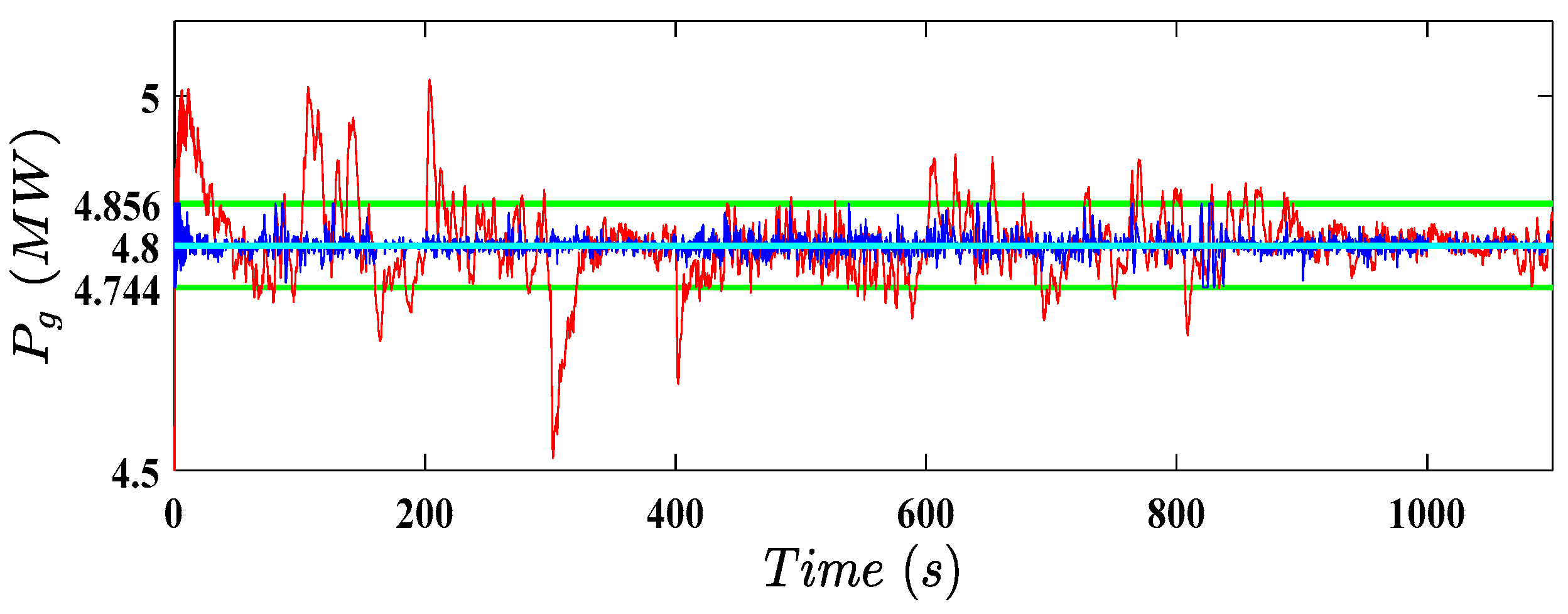
Figure 27.
Generated power using the proposed controller (dark blue line), PID controller (red line), nominal power (light blue line), and constraints (green line), in the fault-free situation, with the second wind speed sequence.
Figure 27.
Generated power using the proposed controller (dark blue line), PID controller (red line), nominal power (light blue line), and constraints (green line), in the fault-free situation, with the second wind speed sequence.
Figure 28.
Generated power using the proposed controller (dark blue line), PID controller (red line), nominal power (light blue line), and constraints (green line), under the second fault scenario, with the second wind speed sequence.
Figure 28.
Generated power using the proposed controller (dark blue line), PID controller (red line), nominal power (light blue line), and constraints (green line), under the second fault scenario, with the second wind speed sequence.
Table 1.
Wind turbine benchmark model parameters.
Table 1.
Wind turbine benchmark model parameters.
| | | | |
| 1.225 | 57.5 | 390 | 55 | 2.7 |
| | | | |
| 945 | 3.034 | 27.8 | 95 | 0.97 |
| | | | |
| 484 | 66.7 | 2.55 | 0.92 | 11.11 |
| | | | |
| 0.6 | −10°/s | 10 | −2 | 30 |
| | | | Full load region |
| 4.8 | 32.107 | 162.5 | 1.71 | 12.3 |
| | | | |
| | | | |
Table 2.
Pitch actuator dynamic change (Data from [
4]).
Table 2.
Pitch actuator dynamic change (Data from [
4]).
| Situation | Fault Indicator | | |
|---|
| Normal Situation | | | |
| Pump Wear | | | |
| Hydraulic Leak | | | |
| High Air Content | | | |
Table 3.
Performance metrics in the fault-free situation.
Table 3.
Performance metrics in the fault-free situation.
| Performance Metrics | Proposed Controller | PID Controller | Unit |
|---|
| 138.9 | 2266 | |
| 400.7 | 2256 | |
| 0.056 | 0.2937 | |
| 0.001331 | 0.001416 | |
| 29.37 | 30 | |
| 10 | 9.79 | |
Table 4.
First fault scenario.
Table 4.
First fault scenario.
| Fault Type | Fault Effect | Fault Period |
|---|
| Pitch actuator pump wear | | |
| Pitch actuator hydraulic leak | | |
| Pitch angle bias | | |
| Pitch actuator high air | | |
| Pitch actuator effectiveness loss | | |
| Aerodynamic characteristic change | | |
Table 5.
Performance metrics with the first fault scenario.
Table 5.
Performance metrics with the first fault scenario.
| Performance Metrics | Proposed Controller | PID Controller | Unit |
|---|
| 155 | 2552 | |
| 414.8 | 2506 | |
| 0.056 | 0.2941 | |
| 0.001349 | 0.001438 | |
| 29.26 | 30 | |
| 10 | 10 | |
Table 6.
Fault identification indices.
Table 6.
Fault identification indices.
| Time (s) | Fault Type | High Air Content | Hydraulic Leak | Pump Wear | Fault-Free | |
|---|
| RMSE | VAF | RMSE | VAF | RMSE | VAF | RMSE | VAF |
|---|
| 0–200 | Fault-Free | 0.37 | −788 | 0.36 | −842 | 0.39 | −5916 | 0.43 | 99.98 | 0 |
| 200–300 | Pump Wear | 3.25 | 50.94 | 1.94 | 66.65 | 0.15 | 98.91 | 1.46 | 215.1 | 0 |
| 300–400 | Fault-Free | 0.31 | −890 | 0.31 | −932 | 0.33 | −6291 | 0.37 | 97.65 | 0 |
| 400–500 | Hydraulic Leak | 2.40 | 75.01 | 0.19 | 99.26 | 67.99 | 2.4 | 2.54 | 575.7 | 0 |
| 500–600 | Fault-Free | 0.35 | −921 | 0.34 | −963 | 0.37 | −6420 | 0.41 | 99.86 | 0 |
| 600–700 | Pitch Bias | 27.82 | −41.85 | 21.99 | −32.33 | 18.67 | −24.33 | 87.62 | 4.05 | 5 |
| 700–800 | Fault-Free | 6.24 | −93370 | 6.20 | −68300 | 6.24 | −182000 | 6.35 | 97.85 | 0 |
| 800–900 | High Air Content | 0.42 | 97.50 | 1.81 | 76.41 | 1.64 | 79.01 | 1.95 | 383.5 | 0 |
| 900–1000 | Fault-Free | 0.53 | −866 | 0.41 | −923 | 0.44 | −6309 | 0.05 | 99.89 | 0 |
| 1000–1100 | Effectiveness loss | 19.14 | −903 | 18.7 | −5800 | 19.56 | −16700 | 21.05 | 1100 | 0 |
| 1100–1200 | Fault-Free | 1.71 | −8870 | 1.67 | −5990 | 1.75 | −17300 | 1.88 | 99.17 | 0 |
| 1200–1300 | Aerodynamic change | 0.29 | −751.6 | 0.28 | −807.9 | 0.31 | −5770 | 0.34 | 11.89 | 0 |
| 1300–1500 | Fault-Free | 0.46 | −755 | 0.46 | −811 | 0.49 | −5790 | 0.54 | 98.38 | 0 |
Table 7.
Second fault scenario.
Table 7.
Second fault scenario.
| Fault Type | Fault Effect | Fault Period |
|---|
| Pitch actuator pump wear | | |
| Pitch actuator effectiveness loss | | |
| Pitch actuator hydraulic leak | | |
| Pitch angle bias | | |
| Pitch actuator high air | | |
| Aerodynamic characteristic change | | |
Table 8.
Performance metrics in the fault-free situation, with the second wind speed sequence.
Table 8.
Performance metrics in the fault-free situation, with the second wind speed sequence.
| Performance Metrics | Proposed Controller | PID Controller | Unit |
|---|
| 212.5 | 1762 | |
| 465 | 1817 | |
| 0.056 | 0.2094 | |
| 0.001299 | 0.001371 | |
| 29.12 | 30 | |
| 10 | 7.46 | |
Table 9.
Performance metrics under the second fault scenario, with the second wind speed sequence.
Table 9.
Performance metrics under the second fault scenario, with the second wind speed sequence.
| Performance Metrics | Proposed Controller | PID Controller | Unit |
|---|
| 304.2 | 3747 | |
| 544.9 | 3549 | |
| 0.056 | 0.2214 | |
| 0.001421 | 0.001376 | |
| 29.40 | 30 | |
| 10 | 10 | |


