Power Quality Disturbances Classification via Fully-Convolutional Siamese Network and k-Nearest Neighbor

Abstract

The classification of disturbance signals is of great significance for improving power quality. The existing methods for power quality disturbance classification require a large number of samples to train the model. For small sample learning, their accuracy is relatively limited. In this paper, a hybrid algorithm of k-nearest neighbor and fully-convolutional Siamese network is proposed to classify power quality disturbances by learning small samples. Multiple convolutional layers and full connection layers are used to construct the Siamese network, and the output result of the Siamese network is used to judges the category of the signal. The simulation results show that: For small sample sizes, the accuracy of the proposed approach is significantly higher than that of the existing methods. In addition, it has a strong anti-noise ability.

1. Introduction

With the development of smart grids, the large-scale integration of advanced power electronic devices, renewable energies, and electric vehicles have brought new challenges to the operation of distribution networks. For example, the uncertainty of photovoltaic output power easily causes a voltage drop in the distribution network [1]. Similarly, the fluctuation and intermittence of wind farms’ produced power may cause the voltages of the distribution network to exceed the limits, since the wind power lies on the wind speed that varies from time to time [2]. The unstable power quality will seriously affect industrial production and residential electricity consumption, and even threaten the safe and stable operation of the power system. How to improve power quality has become a common concern of power companies and power users. The premise of improving power quality is to distinguish the category of disturbance quickly for massive high-dimensional power quality data.

Power quality disturbances classification mainly consists of feature extraction and pattern recognition. The quality of the features has a major impact on the accuracy of the classification. The traditional processing methods for feature extraction mainly include wavelet transform, fast Fourier transform, s-transform, and Hilbert–Huang transform. Wavelet transform can be used to analyze the time-frequency characteristics of signals and it is suitable for the analysis of non-stationary signals with sudden change characteristics. However, it is sensitive to noise, and the choice of basis function depends on experts’ experience [3,4]. Fast Fourier transform has the advantage of low computation, which makes it widely used in the field of signal processing. It is only suitable for the analysis of stationary signals, and cannot deal with power quality disturbance signals with non-stationary characteristics such as transient and sudden change [5]. As an extension of wavelet transform and short-time Fourier transform, the height and width of window function of s-transform vary with frequency, which overcomes the shortcoming of short-time Fourier transform with fix height and width of the window function. Nevertheless, s-transform is insensitive to the detection of singularities in signals, and the computational complexity is high [6,7]. Hilbert–Huang transform is good at dealing with nonlinear and non-stationary power quality disturbance signals, but it has the problem of endpoint effect and modal aliasing [8]. Generally speaking, these traditional methods rely on experience to select features. There is no unified theoretical basis for extracting features, and the summarized features are not universal. For different data sets, the quality of classification is difficult to guarantee.

Pattern recognition uses the extracted features to determine the category of power quality disturbances data. Common methods include support vector machine (SVM), Bayesian classification, k-nearest neighbor method, case-based reasoning, and multi-layer perceptron (MLP). SVM is suitable for binary classification. For n categories of power quality disturbances, n SVM needs to be trained. Each SVM needs to use all the training set. Therefore, the training speed of SVM decreases sharply with the increase of the training set, which makes it difficult to process large sample data sets [9,10]. Bayesian classification is sensitive to the form of input data, and the prior probability depends on the hypothesis, which may lead to poor classification results due to the inaccurate prior model [11]. The k-nearest neighbor algorithm is simple to implement. When the number of training samples and the dimension of feature vectors are large, the algorithm’s complexity will be very high. In addition, the K value that has a great impact on the results needs to be set artificially [12]. Case-based reasoning requires a large amount of historical data, and all kinds of disturbance scenarios should also be included in the database [13]. Multilayer perceptron has powerful non-linear mapping ability and can fit arbitrary continuous functions theoretically. However, it is prone to over-fitting [14]. In general, due to the high dimensionality of the power quality disturbances data, the accuracy of the traditional methods for pattern recognition is low, and it is difficult to meet the actual demand.

In recent years, deep learning technology has become one of the most popular research fields of artificial intelligence, and it has made great achievements in the fields of the power system such as load curve modeling, photovoltaic power prediction, and fault diagnosis. Specifically, many scholars have tried to apply some deep neural networks to improve the accuracy of power quality disturbance classification. For example, the stack sparse auto-encoder is proposed to automatically extract the feature of power quality disturbances data in [15]. The simulation result shows that the stack sparse auto-encoder can effectively learn the natural characteristics of data by reducing dimensionality. To improve the accuracy of classification, a novel framework consists of convolutional neural networks and other classifier is presented in [16,17]. While in [18], the s-transform is used to obtain the specific features, and then the categories of power quality disturbances are determined by a probabilistic neural network. Although the accuracy of these deep neural networks is high, the training process requires a large number of samples which are difficult to obtain in some distribution networks. Siamese network is a typical neural network for few-shot learning. It can automatically determine the categories of samples by calculating similarity, which is very suitable for classification using a few samples from the training set. At present, effective applications based on the Siamese network focus on data classification such as signatures recognition [19,20], disease diagnosis [21] and object tracking [22]. To the best of our knowledge, there is no report on the use of the Siamese network to classify power quality disturbances.

The above analyses brings us to a summary: although traditional methods (e.g., SVM) are suitable for small sample learning, their accuracy is low. Some deep neural networks such as convolutional neural networks (CNN) have relatively high accuracy, but they need a large number of samples for training models. How to design a novel method with high accuracy by learning small samples deserves further study.

In order to address these issues, a hybrid algorithm of k-nearest neighbor and fully-convolutional Siamese network is proposed to classify power quality disturbances. The key contributions of this paper mainly include:

• This is the first exploration of the application of the hybrid algorithm of k-nearest neighbor and fully-convolutional Siamese network in power quality disturbances. The proposed approach only requires a few samples to train the model, and the accuracy is higher than the traditional method.
• The conventional Siamese network is composed of multiple full connection layers, which leads to its low accuracy. By applying multiple convolutional layers, the Siamese network can automatically extract the intrinsic attributes of power quality disturbance to improve accuracy.
• Unlike most deep neural networks (e.g., CNN and MLP) that train a classifier (e.g., SoftMax) through samples, the Siamese network judges the categories by calculating the distance between two feature vectors, which provides a new idea for power quality disturbance classification.

The rest of this paper is organized as follows. Section 2 introduces the generation of data sets. Section 3 explains the principle of the Siamese network and its application in power quality disturbance. Section 4 tests the performance of the proposed approaches through simulation. Section 5 summarizes the work and results of this paper.

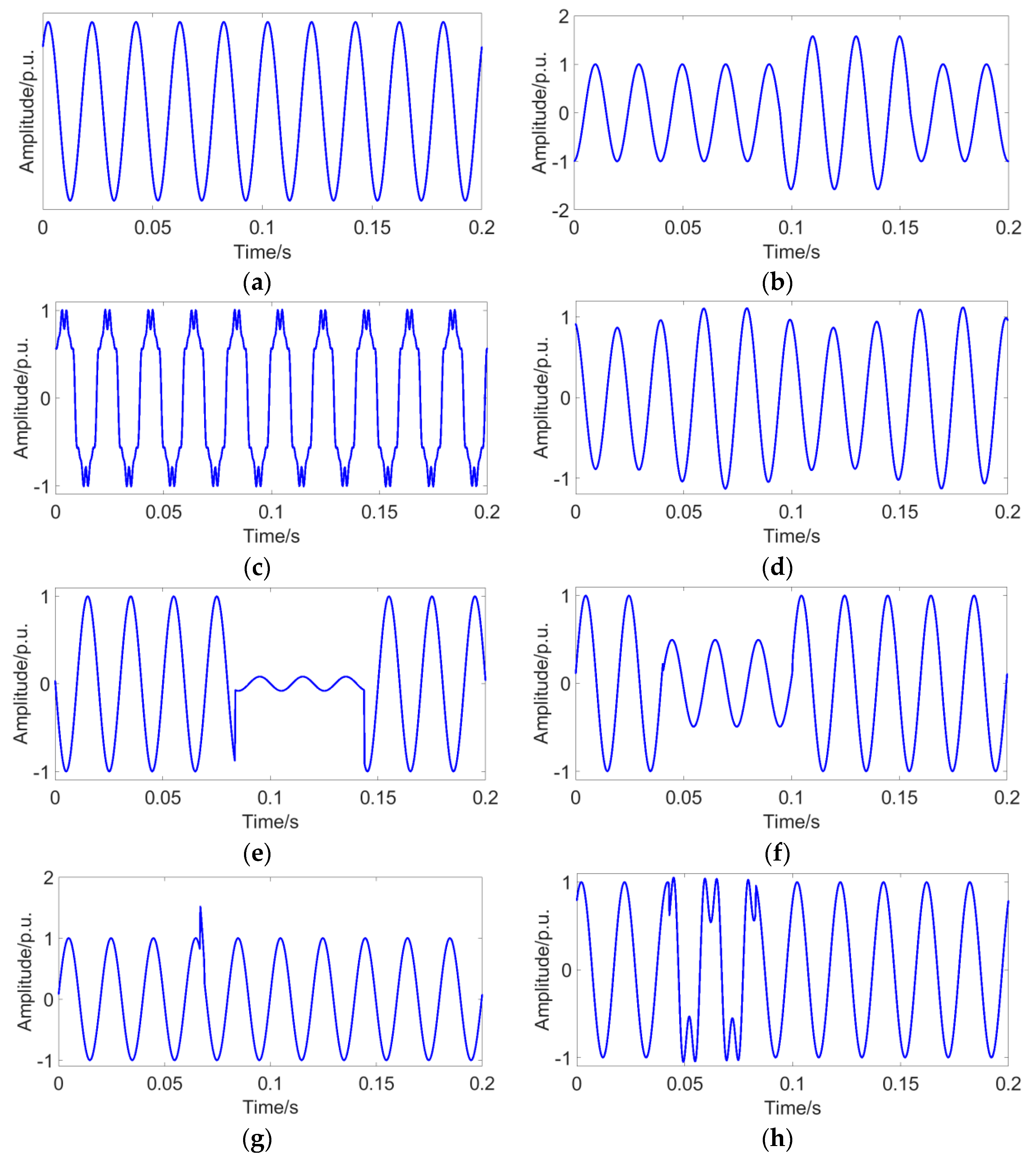
2. Data Set Generation

Most of the existing literature get data sets through simulation since it is difficult to obtain the actual data of power quality disturbance. Various power quality disturbances are defined in the IEEE standard 1159 [23]. This paper considers seven classical power quality disturbance signals, including swell, sag, harmonic, flicker, interruption, spike and oscillatory transient. Their mathematical formulas are shown in

Table 1. Mathematical formulas of power quality disturbances.

Symbol	Type of Disturbance	Equations	Parameters
C1	Normal sine	$z=A\sin wt$	$T$ = 0.02 s, $w=2\pi f$
C2	Swell	$z=A[1+\alpha (u(t-t_1)-u(t-t_2))]\sin wt$	$0.1\le \alpha <0.8$,$T\le t_2-t_1\le 9T$
C3	Harmonic	$\begin{array}{l}z=A(\sin wt+{\alpha }_3\sin 3wt+{\alpha }_5\sin 5wt+\\ {\alpha }_7\sin 7wt+{\alpha }_{11}\sin 11wt)\end{array}$	$0.05\le {\alpha }_i\le 0.15$
C4	Flicker	$z=A(1+\alpha \sin \beta wt)\sin wt$	$0.1\le \alpha \le 0.2$$0.1\le \beta \le 0.2$
C5	Interruption	$z=A[1-\alpha (u(t-t_1)-u(t-t_2))]\sin wt$	$0.9\le \alpha <1.0$$T\le t_2-t_1\le 9T$
C6	Sag	$z=A[1-\alpha (u(t-t_1)-u(t-t_2))]\sin wt$	$0.1\le \alpha <0.9$$T\le t_2-t_1\le 9T$
C7	Spike	$z=A[1-(u(t-t_1)-u(t-t_2))]\sin wt$	$T/20\le t_2-t_1\le T/10$
C8	Oscillatory transient	$z=\alpha e^{-c(t-t_1)}[u(t-t_1)-u(t-t_2)]\sin \beta wt+\sin wt$	$0.1\le \alpha \le 0.8$$T\le t_2-t_1<3T$

, where $T$ is 0.02, $\alpha$ is a random number within the thresholds. The above power quality disturbance signals are visualized as shown in Figure 1.

3. Methodology

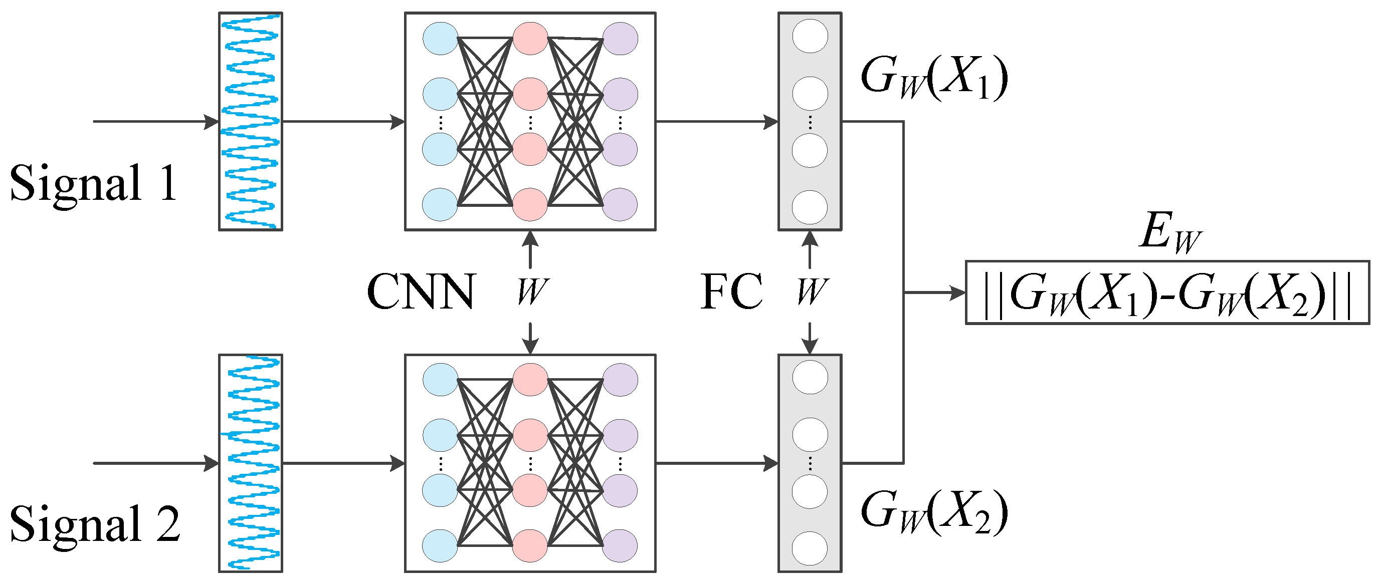
3.1. Siamese Network

The traditional method for power quality disturbance classification is to use a classifier, such as CNN and SVM. These methods are not suitable for the application of power quality disturbance classification where the number of categories is large and the number of samples per category is small. The Siamese network is a kind of distance-based method used for solving this problem. It calculates the similarity metric between the power quality disturbances signals to be classified and a database of stored prototypes. This similarity metric was used to match new power quality disturbances signals from previously-unused categories during training.

The core idea of the Siamese network is to map the power quality disturbance signal to the target space through a function, and compare the similarity in the target space using simple distance (e.g., Euclidean distance). Specifically, the given a series of functions, $G_W(X)$ are parameterized by W. The goal of the training process is to find the optimal parameters $W$ so that the similarity is large when $X_1$ and $X_2$ belong to different disturbances categories and small when they are the same disturbance category. In the training phase, two samples are selected as a pair of inputs data for the Siamese network [24,25,26].

As shown in Figure 2, the Siamese framework has a symmetrical structure where the neural networks share weights to process power quality disturbance signals.

Let $X_1$ and $X_2$ present a pair of power quality disturbance signals. $Y$ is a binary label for a pair of signals. If $X_1$ and $X_2$ belong to the same category of disturbance, $Y$ equals 1. On the contrary, if $X_1$ and $X_2$ do not belong to the same category of disturbance, $Y$ equals 0. $W$ represents the shared weight vector of deep neural networks (e.g., CNN and MLP). The $G_W(X_1)$ and $G_W(X_2)$ are the variables generated by mapping $X_1$ and $X_2$ into low-dimensional space. The similarity of $X_1$ and $X_2$ in low-dimensional space is measured by the energy function. Its mathematical formula is as follows:

$$E_W(X_1,X_2)=\Vert G_W(X_1)-G_W(X_2)\Vert .$$

(1)

The contrastive loss function relies on samples and the parameters of the energy function. Its mathematical formula is:

$$Loss(W)={\displaystyle \sum _{i=1}^{P}L\left(W,{\left(Y,X_1,X_2\right)}^i\right)}$$

(2)

$$L\left(W,{\left(Y,X_1,X_2\right)}^i\right)=\left(1-Y\right)L_G\left(E_W{\left(X_1,X_2\right)}^i\right)+Y{L}_I\left(E_W{\left(X_1,X_2\right)}^i\right),$$

(3)

where $P$ is the number of samples in the training set. ${\left(Y,X_1,X_2\right)}^i$ is the i-th sample that includes a pair of power quality disturbance signals and a label (same or fake). $L_G$ is the loss function for a pair of signals from the same category. $L_I$ is the loss function for a pair of signals from different categories. $L$ will increase the energy function of different pairs and decrease the energy function of the same pairs. In order to achieve this, $L_G$ is designed as a monotonically increasing function, and $L_I$ is designed as a monotonically decreasing function. In this paper, the exact loss function for a single sample is designed as follows:

$$L(W,Y,X_1,X_2)=\left(1-Y\right)\frac{2}{Q}{\left(E_W\right)}^2+Y2Q{e}^{-\frac{2.77}{Q}{E}_W},$$

(4)

where $Q$ is a constant and the loss function is convergent. The concrete proof can be seen in [25].

3.2. Convolutional Network

The convolutional network has been widely used in image classification, target detection, and style transfer because of its powerful feature extraction ability [27,28,29]. In this paper, an important contribution of the proposed approach is that the convolutional network is used to extract representations that are robust to geometric distortions of the input data.

The convolutional network consists of an input layer, convolutional layer, pooling layer, and output layer. The operation of the convolutional layer is shown in Figure 3. The convolutional layer convolutes the signal matrix from the input layer and adds the bias vector to output the feature map through the activation function. The relationship of dimension is as follows: $m=n-k+1$. The mathematical formula of the convolutional layer is as follows:

$$x_i=f(x_{i-1}\ast w_i+b_i),$$

(5)

where $w_i$ denotes the weight of convolutional kernel in i-th layer. $x_i$ is the output value of in i-th convolutional layer and b_i is the bias vector in i-th convolutional layer. $\ast$ denotes the operation of convolution and denotes the activation function. The activation function is used to transform data nonlinearly so that the neural network can fit the complex nonlinear relationship. Common activation functions include sigmoid, hyperbolic tangent and rectified linear unit. When the input value is large, the output of Sigmoid and hyperbolic tangent functions are close to 0. In this case, with the increase of the number of hidden layers, the error is difficult to continue to propagate downwards and the gradient disappears easily. For this reason, the rectified linear unit will be used as the activation function in the convolutional layer.

The pooling layer compresses and maps the feature map from the convolutional layer to reduce the computational complexity and dimension of the feature. The features generated by pooling layer have the invariant properties of rotation and can prevent the over-fitting to a certain extent. As shown in Figure 4, the size of the feature map decreases after being processed by the pooling layer, and the relationship of dimensions among input data, pooling matrix, and output data are as follows: $m=n/k$. The mathematical formula of pooling layer is as follows:

$$x_i={\beta }_i\mathrm{subdown}(x_{i-1})+b_i,$$

(6)

where “subdown“ is subsampled function. ${\beta }_i$ and $b_i$ are bias vectors. In this paper, the pooling layer will select the max-pooling function.

3.3. K-Nearest Neighbor

The input of the Siamese network is a pair of power quality disturbance signals, and its output is the distance between the two signals. Usually, we need to make many pairs of unknown signals and known signals that are fed to the Siamese network. Then, we divide the unknown signals into the kind of known signal with the shortest distance from it. This traditional method will be affected by noise, resulting in the accuracy of the Siamese network decline. Therefore, the k-nearest neighbor is proposed to improve the accuracy of the Siamese network. Its steps are as follows:

(1) For an unknown signal, it is combined with the known signal from the training set into $n$ pairs. The $n$ is the number of samples in the training set. These $n$ pairs of signals are fed to the Siamese network, and the distance between the unknown signal and $n$ samples is output by the Siamese network.

(2) The $n$ samples are listed in descending order by distance. The first $k$ samples are selected, and the number of categories of $k$ samples is counted. Finally, the unknown signal is assigned to the largest number of categories.

3.4. Process of the Proposed Method

To summarize the above analysis, the steps for power quality disturbances classification based on Siamese network are as follows:

(1) Format transformation: as is known to all, the original purpose of designing these deep neural networks is to classify images, which have the same size of row and column. However, the power quality disturbance signal is a one-dimensional time series, which cannot be directly used as the input data of the deep neural network. Therefore, it is necessary to convert the power quality disturbance signal into a two-dimensional matrix with the same size of row and column. Take the signal containing 140 elements as an example to explain the principle of format transformation Firstly, some zero elements are added to the tail of the time series to make it become a vector with 144 elements. Then, the time series is transformed into a matrix of 12 × 12 scales as input data of the Siamese network.

(2) Data normalization: after format transformation, power quality disturbance signals need to be normalized, and otherwise the loss function may not converge. In this paper, the input data is transformed into standard data that range from 0 to 1 by the min-max normalization method.

(3) Updating network parameters: after normalization, the convolution neural network maps the two signals to low-dimensional vectors. Then, the similarity between the two signals is calculated to update the weight of the Siamese network via the chain rule and gradient descent method.

(4) Obtain the results: after training the network, comparing an unknown signal against samples of labeled signals, we are able to determine the labeled signal which is most similar to the unknown signals and obtains a classification result.

The program of power quality disturbances classification via the Siamese network is designed with multiple stages: (1) define network, (2) share weights, (3) train network, (4) predict class. Part of the code is shown in

Table 2. The program of power quality disturbances classification via Siamese network.

Program

# 1.Define network base_network = create_base_network(input_shape) input_a = Input(shape=input_shape) input_b = Input(shape=input_shape) # 2.Share weights processed_a = base_network(input_a) processed_b = base_network(input_b) distance = Lambda(euclidean_distance,output_shape=eucl_dist_output_shape)([processed_a, processed_b]) model = Model([input_a, input_b], distance) # 3.Train network rms = RMSprop() model.compile(loss=contrastive_loss, optimizer=rms, metrics=[accuracy]) model.fit([tr_pairs[:, 0], tr_pairs[:, 1]], tr_y,batch_size=128,epochs=epochs,validation_data=([te_pairs[:, 0], te_pairs[:, 1]],te_y)) # 4. Predict class y_pred = model.predict([te_pairs[:, 0], te_pairs[:, 1]])

.

4. Case Study

4.1. Architecture and Parameters

The sampling frequency of power quality disturbance data is 3916 Hz, and the sampling time is 10 cycles, namely 784 points per sample. The proportion of training set to the data set is 80%, and the proportion of validation set and test set is 10%. The proposed methods will run under MATLAB2018a and Keras which is a deep learning library. The parameters of the computer are: 6 GB of memory, the processor is dual-core 2.4 GHz and Intel Core i3-3110M.

The architecture and parameters of the Siamese network are shown in

Table 3. Parameters of the Siamese network.

Layer	Parameters	Layer	Parameters
Conv2D	filters = 16, kernel = 5 × 5, ReLU	MaxPooling2D	Pool size = 2 × 2
MaxPooling2D	Pool size = 2 × 2	Dropout	Rate = 0.25
Dropout	Rate = 0.25	Flatten	null
Conv2D	Filters = 36, kernel = 5 × 5, ReLU	Dense	Units = 128

and Figure 5. In addition, the CNN, MLP, SVM, extreme gradient boosting (XGBoost) method and light gradient boosting machine (LightGBM) method are used as baselines to verify the performance of the proposed Siamese network. Their parameters and structures are as follows:

(1) As far as MLP is concerned, the number of neurons in the input layer is 784, and the number of neurons in the middle layer is 500 and 200, respectively. The number of neurons in the output layer is equal to the number of categories. To prevent over-fitting, a dropout layer with a rate of 0.25 is inserted between each full connection layer. The loss function is cross-entropy and the optimizer is the root mean square prop (RMSprop). (2)The CNN consists of two convolutional layers, two Max-Pooling layers, two dropout layers and two full connection layers. The size of kernel in the convolutional layers is 5. The value of the dropout layer is 0.25. The size of pool in max-pooling layers is 2. The number of neurons in the full connection layers is 128 and 8, respectively. (3) For SVM, the fitcecoc function from MATLAB2018a is used to classify power quality disturbances. (4) For XGBoost, the gamma is 0.1. The max depth is 6 and the subsample is 0.7. The min child weight is 3 and eta is 0.1. (5) For LightGBM, its specific parameters are shown in

Table 4. Parameters of LightGBM.

Variable	Value	Variable	Value	Variable	Value	Variable	Value
Boosting type	gbdt	reg_alpha	1	learning_rate	0.01	feature_fraction	0.9
objective	multiclassova	num_leaves	63	bagging_seed	0	bagging_fraction	0.9
metric	multi_error	reg_lambda	2	lambda_l1	0	bagging_freq	01
num_threads	8	lambda_l2	1	verbose	−1	num class	8

. (6) After many experiments, when k is equal to 20, the performance of the proposed method is the best.

Figure 6 shows the training process of the Siamese network. As the number of iterations increases, the loss functions of the training set and validation set decrease. When the number of iterations is more than 120, the loss function of the neural network tends to be stable, which indicates that the network has converged. The loss function of validation set is very close to that of test set, which indicates that the Siamese network has strong generalization performance.

4.2. Simulation Results

In order to analyze the influence of data size on the performance of the proposed method, simulation was carried out in seven cases that are shown in

Table 5. The number of samples in different cases.

Cases	Training Set	Validation Set	Test Set	Total
Case 1	80	40	40	160
Case 2	160	64	64	288
Case 3	400	56	56	512
Case 4	800	112	112	1024
Case 5	1600	224	224	2048
Case 6	3200	448	448	4096
Case 7	6400	896	896	8192

. Each case was run 30 times independently and their average accuracy is obtained as shown in

Table 6. The accuracy of different cases.

Approaches	Case 1	Case 2	Case 3	Case 4	Case 5	Case 6	Case 7
Proposed method	81.25%	84.82%	94.79%	98.22%	97.99%	98.70%	98.09%
MLP	37.50%	39.06%	32.14%	46.42%	52.23%	65.87%	80.24%
CNN	57.50%	68.75%	91.07%	98.12%	98.21%	98.43%	99.21%
SVM	22.50%	18.75%	16.07%	18.75%	19.19%	18.97%	24.55%
XGBoost	35.00%	34.38%	60.71%	73.21%	80.36%	85.94%	89.73%
LightGBM	42.50%	43.75%	64.29%	73.21%	83.04%	87.72%	91.18%

.

In order to analyze the performance of the proposed methods under different signal-to-noise ratios (SNR), the original power quality disturbance signals and Gauss white noises are combined to form new samples as shown in Figure 7. Each case is tested 30 times independently, and the average accuracy of each case under each SNR is counted as shown in

Table 7. The accuracy of proposed methods under different SNR.

SNR/dB	Case 1	Case 2	Case 3	Case 4	Case 5	Case 6	Case 7
15	76.88%	80.36%	89.50%	91.46%	91.81%	92.50%	93.75%
25	78.44%	81.25%	92.71%	93.75%	95.83%	95.34%	96.40%
35	79.06%	82.14%	92.70%	95.67%	96.06%	97.39%	97.61%
45	80.34%	84.29%	94.73%	96.73%	97.61%	97.61%	97.72%

and

Table 8. The accuracy of different methods in case 3.

SNR/dB	Proposed Method	MLP	CNN	SVM	XGBoost	LightGBM
15	89.50%	24.07%	86.78%	26.79%	37.50%	37.50%
25	92.71%	26.43%	88.43%	16.07%	55.36%	57.14%
35	92.70%	30.36%	89.11%	25%	53.57%	57.14%
45	94.73%	32.86%	90.46%	16.07%	53.57%	62.50%

.

In order to analyze the performance of the proposed methods under different sampling frequency, each algorithm is repeated 30 times at different frequencies, and the average accuracy is shown in

Table 9. The average accuracy of different methods.

F/Hz	Proposed Method	MLP	CNN	SVM	XGBoost	LightGBM
715	84.38%	39.29%	87.50%	19.64%	60.71%	60.71%
1275	88.54%	41.07%	83.93%	21.43%	51.79%	55.36%
1995	90.62%	48.21%	87.50%	21.43%	44.64%	48.21%
2875	92.97%	35.71%	87.50%	32.14%	55.36%	60.71%
3915	94.79%	32.14%	91.07%	16.07%	60.71%	64.29%

.

4.3. Discussion of Results

The following conclusions can be drawn from Table 6: (1) obviously, the accuracy of the existing methods is less than 70% in cases 1 and 2. The accuracy of the proposed method is higher than 80%, which indicates that the proposed method had clear superiority in power quality disturbances classification with small samples. (2) As the number of samples increases, the accuracy of each algorithm increases. It shows that increasing the number of samples was helpful for improving the accuracy. For a large sample size, the accuracy of the proposed method is very close to that of CNN, and it is much higher than that of other methods. (3) Generally speaking, the proposed method had the best performance, followed by CNN. The performance of XGBoost and LightGBM is similar. SVM has the worst effect.

The following conclusions can be drawn from Table 7 and Table 8: (1) When the signal-to-noise ratio is 15, the accuracy of XGBoost and LightGBM decreases significantly, which indicates that their anti-noise ability is weak. (2) The accuracy of MLP and SVM under different SNR is relatively low, which indicates that they are not suitable for classifying power quality disturbances with noises. (3) In contrast, the accuracy of proposed methods and CNN under different SNR in case 3 is more than 85%, which shows that they have strong robustness. In addition, the accuracy of the proposed methods is slightly higher than that of CNN.

The following conclusions can be drawn from Table 9: obviously, the accuracy of the proposed methods has a positive correlation with the sampling frequency. When the sampling frequency is 715 Hz, the accuracy of the proposed methods is slightly lower than that of CNN, which indicates that the proposed method is suitable for power quality disturbance signals with high sampling frequency. When the sampling frequency is more than 1275 Hz, the accuracy of the proposed methods is higher than that of other methods.

5. Conclusions

The classification of disturbance signals is of great significance for improving power quality and system operation. In this paper, a hybrid algorithm of k-nearest neighbor and fully-convolutional Siamese network is proposed to classify power quality disturbances by learning small samples. The following conclusions are obtained through simulation:

(1) For larger sample sizes, the accuracy of the proposed methods is very close to that of CNN, and higher than that of other traditional methods. For small sample sizes, the accuracy of the proposed method is significantly higher than that of the existing methods (e.g., MLP, CNN, SVM, XGBoost and LightGBM), which shows that the proposed method is very suitable for power quality disturbance classification with a small number of samples.

(2) If the data size is small, the accuracy of the proposed method is higher than that of the traditional methods (e.g., MLP, CNN, SVM, XGBoost and LightGBM) under different SNR. Besides, both the proposed method and CNN show strong anti-noise ability.

(3) The accuracy of the proposed method has a positive correlation with the sampling frequency. In order to ensure the accuracy of the proposed method is high enough, the sampling frequency of the power quality disturbance signal is better than 1275 Hz.

References

1. Wang, Y.; Liao, W.; Chang, Y. Gated Recurrent Unit Network-Based Short-Term Photovoltaic Forecasting. Energies 2018, 11, 2163. [Google Scholar] [CrossRef] [Green Version]
2. Nieto, A.; Vita, V.; Maris, T.I. Power Quality Improvement in Power Grids with the Integration of Energy Storage Systems. Int. J. Eng. Res. Technol. 2016, 5, 438–443. [Google Scholar]
3. Khokhar, S.; Mohd Zin, A.A.; Memon, A.P.; Mokhtar, A.S. A new optimal feature selection algorithm for classification of power quality disturbances using discrete wavelet transform and probabilistic neural network. Measurement 2017, 95, 246–259. [Google Scholar] [CrossRef]
4. Liu, H.; Hussain, F.; Shen, Y.; Arif, S.; Nazir, A.; Abubakar, M. Complex power quality disturbances classification via curvelet transform and deep learning. Electr. Power Syst. Res. 2018, 163, 1–9. [Google Scholar] [CrossRef]
5. Devadasu, G.; Sushama, M. Identification of Voltage Quality Problems under Different Types of Sag/Swell Faults with Fast Fourier Transform Analysis. In Proceedings of the 2nd International Conference on Advances in Electrical, Electronics, Information, Communication and Bio-Informatics (AEEICB), Chennai, India, 27–28 February 2016; pp. 464–469. [Google Scholar]
6. Zhong, T.; Zhang, S.; Cai, G.; Li, Y.; Yang, B.; Chen, Y. Power Quality Disturbance Recognition Based on Multiresolution S-Transform and Decision Tree. IEEE Access 2019, 7, 88380–88392. [Google Scholar] [CrossRef]
7. Satao, S.R.; Kankale, R.S. A New Approach for Classification of Power Quality Events Using S-Transform. In Proceedings of the International Conference on Computing Communication Control and Automation (ICCUBEA), Pune, India, 12–13 August 2016; pp. 1–4. [Google Scholar]
8. Mishra, M.; Sahani, M.; Rout, P.K. An islanding detection algorithm for distributed generation based on Hilbert–Huang transform and extreme learning machine. Sustain. Energy Grids Netw. 2017, 9, 13–26. [Google Scholar] [CrossRef]
9. Thirumala, K.; Pal, S.; Jain, T.; Umarikar, A.C. A classification method for multiple power quality disturbances using EWT based adaptive filtering and multiclass SVM. Neurocomputing 2019, 334, 265–274. [Google Scholar] [CrossRef]
10. Mohanty, S.R.; Ray, P.K.; Kishor, N.; Panigrahi, B.K. Classification of disturbances in hybrid DG system using modular PNN and SVM. Int. J. Electr. Power Energy Syst. 2013, 44, 764–777. [Google Scholar] [CrossRef]
11. Luo, Y.; Li, K.; Li, Y.; Cai, D.; Zhao, C.; Meng, Q. Three-Layer Bayesian Network for Classification of Complex Power Quality Disturbances. IEEE Trans. Ind. Inform. 2018, 14, 3997–4006. [Google Scholar] [CrossRef]
12. Pan, D.; Zhao, Z.; Zhang, L.; Tang, C. Recursive Clustering K-nearest Neighbors Algorithm and the Application in the Classification of Power Quality Disturbances. In Proceedings of the 2017 IEEE Conference on Energy Internet and Energy System Integration (EI2), Beijing, China, 26–28 November 2017; pp. 1–5. [Google Scholar]
13. Sierra-Fernández, J.M.; Rosa, J.J.G.; Palomares-Salas, J.C.; Agüera-Pérez, A.; Jiménez-Montero, Á. Adaptive Detection and Classificaion System for Power Quality Disturbances. In Proceedings of the 2013 International Conference on Power, Energy and Control (ICPEC), Sri Rangalatchum Dindigul, India, 6–8 Febuary 2013; pp. 525–530. [Google Scholar]
14. Mohod, S.B.; Ghate, V.N. MLP-Neural Network Based Detection and Classification of Power Quality Disturbances. In Proceedings of the 2015 International Conference on Energy Systems and Applications, Pune, India, 30 October–1 November 2015; pp. 124–129. [Google Scholar]
15. Qiu, W.; Tang, Q.; Liu, J.; Teng, Z.; Yao, W. Power Quality Disturbances Recognition Using Modified S Transform and Parallel Stack Sparse Auto-encoder. Electr. Power Syst. Res. 2019, 174, 105876. [Google Scholar] [CrossRef]
16. Shen, Y.; Abubakar, M.; Liu, H.; Hussain, F. Power Quality Disturbance Monitoring and Classification Based on Improved PCA and Convolution Neural Network for Wind-Grid Distribution Systems. Energies 2019, 12, 1280. [Google Scholar] [CrossRef] [Green Version]
17. Cai, K.; Hu, T.; Cao, W.; Li, G. Classifying Power Quality Disturbances Based on Phase Space Reconstruction and a Convolutional Neural Network. Appl. Sci. 2019, 9, 3681. [Google Scholar] [CrossRef] [Green Version]
18. Wang, H.; Wang, P.; Liu, T. Power Quality Disturbance Classification Using the S-Transform and Probabilistic Neural Network. Energies 2017, 10, 107. [Google Scholar] [CrossRef] [Green Version]
19. Çalik, N.; Kurban, O.C.; Yilmaz, A.R.; Yildirim, T.; Durak Ata, L. Large-scale offline signature recognition via deep neural networks and feature embedding. Neurocomputing 2019, 359, 1–14. [Google Scholar] [CrossRef]
20. Masoudnia, S.; Mersa, O.; Araabi, B.N.; Vahabie, A.-H.; Sadeghi, M.A.; Ahmadabadi, M.N. Multi-representational learning for Offline Signature Verification using Multi-Loss Snapshot Ensemble of CNNs. Expert Syst. Appl. 2019, 133, 317–330. [Google Scholar] [CrossRef] [Green Version]
21. Wang, J.; Fang, Z.; Lang, N.; Yuan, H.; Su, M.Y.; Baldi, P. A multi-resolution approach for spinal metastasis detection using deep Siamese neural networks. Comput. Biol. Med. 2017, 84, 137–146. [Google Scholar] [CrossRef] [PubMed] [Green Version]
22. Kashiani, H.; Shokouhi, S.B. Visual object tracking based on adaptive Siamese and motion estimation network. Image Vis. Comput. 2019, 83, 17–28. [Google Scholar] [CrossRef] [Green Version]
23. IEEE. Recommended Practices for Monitoring Electric Power Quality; IEEE Std 1159-1995; IEEE-SASB Coordinating Committees: New York, NY, USA, 1995. [Google Scholar]
24. Bertinetto, L.; Valmadre, J.; Henriques, J.F.; Vedaldi, A.; Torr, P.H.S. Fully-Convolutional Siamese Networks for Object Tracking. In European Conference on Computer Visio; Springer: Cham, The Netherlands, 2016. [Google Scholar]
25. Chopra, S.; Hadsell, R.; Lecun, Y. Learning a Similarity Metric Discriminatively, with Application to Face Verification. In Proceedings of the IEEE Computer Society Conference on Computer Vision and Pattern Recognition, San Diego, CA, USA, 20–26 June 2005; pp. 539–546. [Google Scholar]
26. Hadsell, R.; Chopra, S.; Lecun, Y. Dimensionality Reduction by Learning an Invariant Mapping. In Proceedings of the IEEE Computer Society Conference on Computer Vision and Pattern Recognition, New York, NY, USA, 17–22 June 2006; pp. 1735–1742. [Google Scholar]
27. Fang, L.; Jin, Y.; Huang, L.; Guo, S.; Zhao, G.; Chen, X. Iterative fusion convolutional neural networks for classification of optical coherence tomography images. J. Vis. Commun. Image Represent. 2019, 59, 327–333. [Google Scholar] [CrossRef]
28. Li, S.; Dou, Y.; Niu, X.; Lv, Q.; Wang, Q. A fast and memory saved GPU acceleration algorithm of convolutional neural networks for target detection. Neurocomputing 2017, 230, 48–59. [Google Scholar] [CrossRef]
29. Guo, M.; Jiang, J. A robust deep style transfer for headshot portraits. Neurocomputing 2019, 361, 164–172. [Google Scholar] [CrossRef]
Figure 1. Visualization of various power quality disturbances: (a) normal sine; (b) swell; (c) harmonic; (d) flicker; (e) interruption; (f) sag; (g) spike and (h) oscillatory transient.
Energies 12 04732 g001
Figure 2. Structure of Siamese network for power quality disturbances classification.
Energies 12 04732 g002
Figure 3. Operation of convolutional layer.
Energies 12 04732 g003
Figure 4. Operation of pooling layer.
Energies 12 04732 g004
Figure 5. The architecture of Siamese network for power quality disturbances classification.
Energies 12 04732 g005
Figure 6. The training process of the Siamese network.
Energies 12 04732 g006
Figure 7. Visualization of various power quality disturbance signals with noises. (a) The signal-to-noise ratio is 15; (b) the signal-to-noise ratio is 25; (c) the signal-to-noise ratio is 35; and, (d) the signal-to-noise ratio is 45.
Energies 12 04732 g007