Stream Learning in Energy IoT Systems: A Case Study in Combined Cycle Power Plants
by
 , , and
Jesus L. Lobo
1,* ,
,
Igor Ballesteros
2,
Izaskun Oregi
1,
Javier Del Ser
1,2,3 and
Sancho Salcedo-Sanz
4 1
TECNALIA, Basque Research and Technology Alliance (BRTA), 48160 Derio-Bizkaia, Spain
2
University of the Basque Country UPV/EHU, 48013 Bilbao, Spain
3
Basque Center for Applied Mathematics (BCAM), 48009 Bilbao, Spain
4
Department of Signal Processing and Communications, University of Alcalá, E-28871 Alcalá de Henares, Spain
*
Author to whom correspondence should be addressed.
Energies 2020, 13(3), 740; https://doi.org/10.3390/en13030740
Submission received: 25 November 2019
/
Revised: 10 January 2020
/
Accepted: 3 February 2020
/
Published: 8 February 2020
(This article belongs to the Special Issue Machine Learning and Artificial Intelligence for Power and Energy Networks)
Abstract
:The prediction of electrical power produced in combined cycle power plants is a key challenge in the electrical power and energy systems field. This power production can vary depending on environmental variables, such as temperature, pressure, and humidity. Thus, the business problem is how to predict the power production as a function of these environmental conditions, in order to maximize the profit. The research community has solved this problem by applying Machine Learning techniques, and has managed to reduce the computational and time costs in comparison with the traditional thermodynamical analysis. Until now, this challenge has been tackled from a batch learning perspective, in which data is assumed to be at rest, and where models do not continuously integrate new information into already constructed models. We present an approach closer to the Big Data and Internet of Things paradigms, in which data are continuously arriving and where models learn incrementally, achieving significant enhancements in terms of data processing (time, memory and computational costs), and obtaining competitive performances. This work compares and examines the hourly electrical power prediction of several streaming regressors, and discusses about the best technique in terms of time processing and predictive performance to be applied on this streaming scenario.
1. Introduction
The efficiency of Combined Cycle Power Plants (CCPPs) is a key issue in the penetration of this technology in the electricity mix. A recent report [1] has estimated that, in the next decade, the number of projects involving combined cycle technology will increase by a , and this estimation is mainly based on the high efficiency of CCPPs. The electrical power production prediction in CCPPs encompasses numerous factors that should be considered to achieve an accurate estimation. The operators of a power grid often predict the power demand based on historical data and environmental factors, such as temperature, pressure, and humidity. Then, they compare these predictions with available resources, such as coal, natural gas, nuclear, solar, wind, or hydro power plants. Power generation technologies (e.g., solar and wind) are highly dependent on environmental conditions, and all generation technologies are subject to planned and unplanned maintenance. Thus, the challenge for a power grid operator is how to handle a shortfall in available resources versus actual demand. The power production of a peaker power plant varies depending on environmental conditions, so the business problem is to predict the power production of the peaker as a function of meteorological conditions—since this would enable the grid operator to make economic trade-offs about the number of peaker plants to turn on (or whether to buy usually expensive power from another grid).
The referred CCPP in this work uses two gas turbines (GT) and one steam turbine (ST) together to produce up to more electricity from the same fuel than a traditional simple-cycle plant. The waste heat from the GTs is routed to the nearby two STs, which generate extra power. In this real environment, a thermodynamical analysis compels thousands of nonlinear equations whose solution is near unfeasible, taking too many computational memory and time costs. This barrier is overcome by using a Machine Learning based approach, which is a frequent alternative instead of thermodynamical approaches [2]. The correct prediction of its electrical power production is very relevant for the efficiency and economic operation of the plant, and maximizes the income from the available megawatt hours. The sustainability and reliability of the GTs depend highly on this electrical power production prediction, mainly when it is subjected to constraints of high profitability and contractual liabilities.
This work applies stream regression (SR) algorithms for a prediction analysis of a thermodynamic system, which is the mentioned CCPP. Our work uses some of the most known SR learning algorithms to successfully predict (in an online manner, as opposed to [3] where a traditional non-streaming view is considered) the electrical power production by using a combination of input parameters defined by for GTs and STs (ambient temperature, vacuum, atmospheric pressure, and relative humidity). This work shows how the application of real-time analytics or Stream Learning (SL) fits the purposes of a modern industry in which data flow constantly, analyzing the impact of several streaming factors (which should be considered before the streaming process starts) on the production prediction. It also compares the results represented by several error metrics and time processing of several SRs under different experiments, finding the most recommendable ones in the electrical power production prediction, aside from carrying out a statistical significance study. Therefore, the contributions of this work can be summarized as follows:
- We present a work closer to reality, where fast data can be huge, they are in motion, and closely connected, and where there are limited resources (e.g., time, memory) to process them, such as in an IoT application.
- We follow and present a complete procedure about how to tackle SL challenges in energy IoT systems.
- We offer a comparison of stream learners, due to the fact that under these real-time machine learning conditions we need regression methods that learn incrementally
- Finally, we identify the best technique to be applied in the presented scenario, a real-time electrical power production prediction in a CCPP.
The rest of this work is organized as follows: Section 2 provides a background about the topics of the manuscript. Specifically, it introduces the field of SL and presents the field of power production prediction. In Section 3 materials and methods are presented, whereas Section 4 describes the experimental work. Section 5 presents the results of such experiments. Section 6 provides a discussion of the work, and then Section 7 finalizes by presenting the final conclusions of the work.
2. Related Work
There are different works in the literature undertaken related problems by using Machine Learning approaches. In [3,4] the authors successfully applied several regression methods to predict the full load electrical power production of a CCPP. A different approach for the same goal was investigated in [5], where the authors presented a novel approach using a Particle Swarm Optimization algorithm [6] for training feed-forward neural network to predict the power plant production. In line with this last study, the work in [7] developed a new artificial neural network optimized by particle swarm optimization for dew point pressure prediction. In [8] the authors applied forecasting methodologies, including linear and nonlinear regression, to predict GT behavior over time, which allows planning maintenance actions and saving costs, and also because unexpected stops can be avoided. This work [9] presents a comparison of two strategies for GT performance prediction, using statistical regression as technique to analyze dynamic plant signals. The prognostic approach to estimate the remaining useful life of GT engines before their next major overhaul was overcome in [10], where a combination of regression techniques was proposed to predict the remaining useful life of GT engines. In [11] it was showed that regression models were good estimators of the response variables to carry out parametric based thermo-environmental and exergoeconomic analyses of CCPPs. The same authors were involved in [12] when using multiple polynomial regression models to correlate the response variables and predictor variables in a CCPP to carry out a thermo-environmental analysis. More recently, in [13] it is presented a real-time derivative-driven regression method for estimating the performance of GTs under dynamic conditions. A scheme for performance-based prognostics of industrial GTs operating under dynamic conditions is proposed and developed in [14], where a regression method is implemented to locally represent the diagnostic information for subsequently forecasting the performance behavior of the engine.
Regarding the SL topic, many researches have focused on it due to its mentioned relevance, such as [15,16,17,18,19], and more recently in [20,21,22,23]. The application of regression techniques to SL has been recently addressed in [24], where the authors cover the most important online regression methods. The work [25] deals with ensemble learning from data streams, and specifically it focused on regression ensembles. The authors of [26] propose several criteria for efficient sample selection in case of SL regression problems within an online active learning context. In general, we can say that regression tasks in SL have not received as much attention as classification tasks, and this was spotlighted in [27], where researchers carried out an study and an empirical evaluation of a set of online algorithms for regression, which includes the baseline Hoeffding-based regression trees, online option trees, and an online least mean squares filter.
2.1. Stream Learning in the Big Data Era
The Big Data paradigm has gained momentum last decade, because of its promise to deliver valuable insights to many real-world applications [28]. With the advent of this emerging paradigm comes not only an increase in the volume of available data, but also the notion of its arrival velocity, that is, these real-world applications generate data in real-time at rates faster than those that can be handled by traditional systems. One particular case of the Big Data paradigm is real-time analytics or SL, where sequences of items (data streams), possibly infinite, arrive continuously, and where each item has a timestamp and so a temporal order. Data streams arrive one by one, and we would like to build and maintain models (e.g., predictors) of these items in real-time.
This situation leads us to assume that we have to deal with a potentially infinite and ever-growing datasets that may arrive continuously in batches of instances, or instance by instance, in contrast to traditional systems (batch learning) where there is free access to all historical data. These traditional processing systems assume that data are at rest and simultaneously accessed. For instance, database systems can store large collections of data and allow users to run queries or transactions. The models based on batch processing do not continuously integrate new information into already constructed models but, instead, regularly reconstruct new models from the scratch. However, the incremental learning that is carried out by SL presents advantages for this particular stream processing by continuously incorporating information into its models, and traditionally aim at minimal processing time and space. Because of its ability of continuous large-scale and real-time processing, incremental learning has recently gained more attention in the context of Big Data [29]. SL also presents many new challenges and poses stringent conditions [30]: only a single sample (or a small batch of instances) is provided to the learning algorithm at every time instant, a very limited processing time, a finite amount of memory, and the necessity of having trained models at every scan of the streams of data. In addition, these streams of data may evolve over time and may be occasionally affected by a change in their data distribution (concept drift) [31], forcing the system to learn under non-stationary conditions.
We can find many examples of real-world SL applications [32], such as mobile phones, industrial process controls, intelligent user interfaces, intrusion detection, spam detection, fraud detection, loan recommendation, monitoring and traffic management, among others [33]. In this context, the Internet of Things (IoT) has become one of the main applications of SL [34], since it is producing huge quantity of data continuously in real-time. The IoT is defined as sensors and actuators connected by networks to computing systems [35], which monitors and manages the health and actions of connected objects or machines in real-time. Therefore, stream data analysis is becoming a standard to extract useful knowledge from what is happening at each moment, allowing people or organizations to react quickly when inconveniences emerge or when new trends appear, helping them increase their performance.
A Fog Computing Perspective
Nowadays, cloud computing is already more than a promising paradigm in IoT Big Data analytics. Instead of being only on the cloud, the idea of bringing computing and analytics closer to the end-users/devices was proposed under the name of Fog Computing [36]. Relying on fog-based analytics, we can benefit from the advantages of cloud computing while reducing or avoiding some of its drawbacks, such as network latency or security risks. It has been confirmed [37] that, by hosting data analytics on fog computing nodes, the overall performance can be improved due to the avoidance of transmitting large amounts of raw data to distant cloud nodes. It is also possible to perform real-time analytics to some extent since the fog is hosted locally close to the source of data. Smart application gateways are the core elements in this new fog technology, performing some of the tasks currently done by cloud computing such as data aggregation, classification, integration, and interpretation, thus facilitating the use of IoT local computing resources [38].
2.2. CCPPs and Stream Learning Regression
We have presented in the introduction of this Section how some problems in a CCPP have been tackled by using Machine Learning approaches, concretely applying regression techniques, and mostly from a batch learning perspective. Since the emergence of the SL field, many modern industrial processes based on these approaches are migrating from the traditional batch learning perspective to this real-time Machine Learning paradigm. And it is not surprising due to its benefits in many real cases, where the number of sensors producing data is huge, and the training of the Machine Learning models become unmanageable. Some processes need to be interrupted until Machine learning models are updated or retrained, which may lead to some operational drawbacks such as a loss of efficiency or an increase in costs. However, by applying a SL perspective, it is not required to store all historical data, and the Machine learning models can be trained incrementally every time new data instances arrive without interrupting any industrial process. The power production prediction process based on Machine learning models is not exempt from this inconveniences, and finds in the SL paradigm the suitable solution in a IoT environment.
Therefore the task of power production prediction can be seen as a process based on data streams, as we will show in this work. Even though the work [3] is perfectly adequate under specific conditions which allow a batch processing, and where the author assumed the possibility of storing all the historical data to process it and predict the electrical power generation with a Machine Learning regression algorithms, we tackle the same problem from a contemporary streaming perspective. In this work we have considered a CCPP as a practical case of IoT application, where different sensors provide the required data to efficiently predict in real-time the full load electrical power generation (see Figure 1). In fact, all the data generated by IoT applications can be considered as streaming data since they are obtained in specific intervals of time. Power generation is a complex process, and understanding and predicting power production is an important element in managing a CCPP, and its connection to the power grid.
Our view is close to real system where fast data can be huge, it is in motion, it is closely connected, and where there are limited resources (e.g., time, memory) to process it. While it does not seem appropriate to retrain the learning algorithms every time new instances are available (what occurs in batch processing), a streaming perspective introduces significant enhancements in terms of data processing (less time and computational costs), algorithms training (they are updated every time new instances come), and presents a modernized vision of a CCPP considering it as an IoT application, and as a part of the Industry paradigm [39]. To the best of our knowledge, this is the first time that a SL approach is applied to CCPPs for electrical production prediction. This work could be widely replicated for other streaming prediction purposes in CCPPs, even more, it can serve as a practical example of SL application for modern electrical power industries that need to obtain benefits from the Big Data and IoT paradigms.
3. Materials and Methods
3.1. System Description
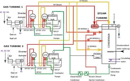
The proposed CCPP is composed of two GTs, one ST and two heat recovery steam generators. In a CCPP, the electricity is generated by GTs and STs, which are combined in one cycle, and is transferred from one turbine to another [40]. The CCPP captures waste heat from the GT to increase efficiency and the electrical production. Basically, how a CCPP works can be described as follows (see Figure 1):
- Gas turbine burns fuel: the GT compresses air and mixes it with fuel that is heated to a very high temperature. The hot air-fuel mixture moves through the GT blades, making them spin. The fast-spinning turbine drives a generator that converts a portion of the spinning energy into electricity
- Heat recovery system captures exhaust: a Heat Recovery Steam Generator captures exhaust heat from the GT that would otherwise escape through the exhaust stack. The Heat Recovery Steam Generator creates steam from the GT exhaust heat and delivers it to the ST
- Steam turbine delivers additional electricity: the ST sends its energy to the generator drive shaft, where it is converted into additional electricity
This type of CCPP is being installed in an increasing number of plants around the world, where there is access to substantial quantities of natural gas [41]. As it was reported in [3], the proposed CCPP is designed with a nominal generating capacity of 480 megawatts, made up of megawatts ABB GTs, dual pressure Heat Recovery Steam Generators and megawatts ABB ST. GT load is sensitive to the ambient conditions; mainly ambient temperature (AT), atmospheric pressure (AP), and relative humidity (RH). However, ST load is sensitive to the exhaust steam pressure (or vacuum, V). These parameters of both GTs and STs are used as input variables, and the electrical power generating by both GTs and STs is used as a target variable in the dataset of this study. All of them are described in Table 1 and correspond to average hourly data received from the measurement points by the sensors denoted in Figure 1.
3.2. The Stream Learning Process
We define a SL process as one that generates on a given stream of training data a sequence of models . In our case stands for labeled training data and is a model function solely depending on and the recent p instances with p being strictly limited (in this work , representing a real case with a very stringent use case of online learning). The learning process in streaming is incremental [15], which means that we have to face the following challenges:
- The stream algorithm adapts/learns gradually (i.e., is constructed based on without a complete retraining),
- Retains the previously acquired knowledge avoiding the effect of catastrophic forgetting [42], and
- Only a limited number of p training instances are allowed to be maintained. In this work we have applied a real SL approach under stringent conditions in which instance storing is not allowed.
Therefore, data-intensive applications often work with transient data: some or all of the input instances are not available from memory. Instances in the stream arrive online (frequently one instance at a time) and can be read at most once, which constitutes the strongest constraint for processing data streams, and the system has to decide whether the current instance should be discarded or archived. Only selected past instances (e.g., a sliding window) can be accessed by storing them in memory, which is typically small relative to the size of the data streams.
A widespread approach for SL is the use of a sliding window to keep only a representative portion of the data, because we are not interested in storing all the historical data, particularly when we must meet the memory space constraint required for algorithms working. This technique is capable of dealing with concept drift, removing those instances that belong to an old concept. According to [43], the training window size can be fixed or variable over time, what can be a challenging task. On the one hand, a short window reflects the current distribution more accurately, thus it can assure a fast adaptation when drift occurs, but during stable periods a too short window worsens the performance of the algorithm. On the other hand, a large window shows a better performance in stable periods, however it reacts to drifts slower. Sliding windows of a fixed size store in memory a fixed number of the w most recent instances. Whenever a new instance arrives, it is stored in memory and the oldest one is discarded. This is a simple adaptive learning method, often referred as forgetting strategy. However, sliding windows of variable size vary the number of instances in a window over time, usually depending on the indications of a change detector. A straightforward approach is to shrink the window whenever a change is detected, such that the training data reflects the most recent concept, and grow the window otherwise. This work is not focused on concept drift, so we do not use any sliding window (except in the case of RHAT as we will see in Section 3.3), but we train and test our algorithms only with the arriving instance by using a test-then-train evaluation (see Section 4.2). This is the so-called online learning where only one instance is processed at each time.
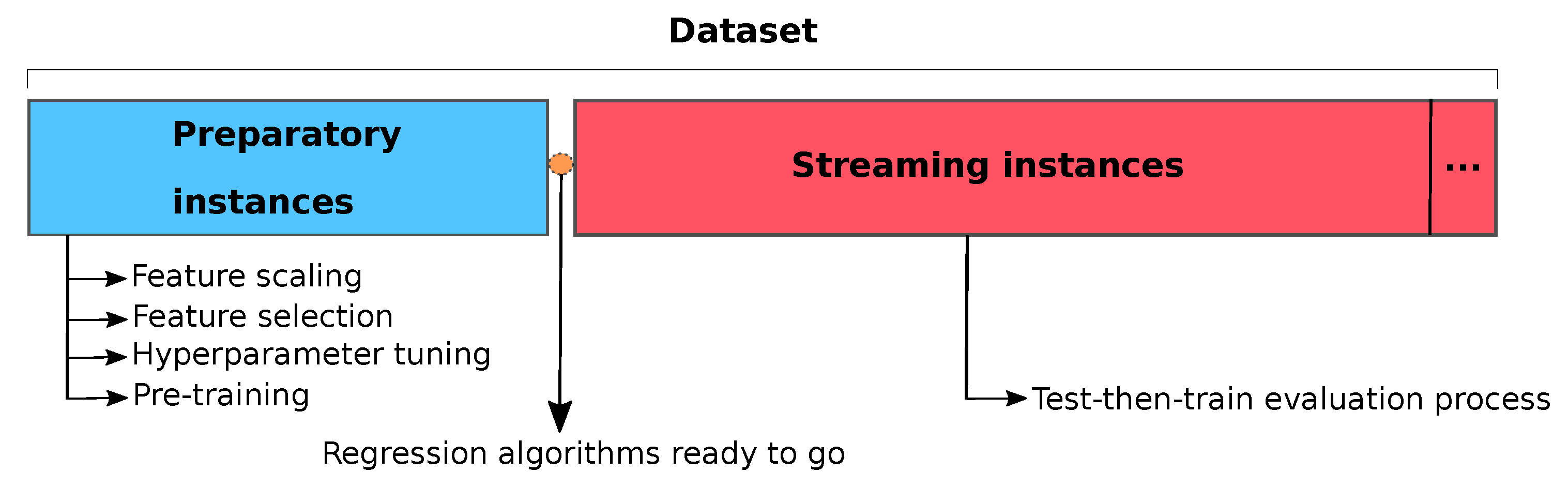
When designing SL algorithms, we have to take several algorithmic and statistical considerations into account. For example, we have to face the fact that, as we cannot store all the inputs, we cannot unwind a decision made on past data. In batch learning processing we have free access to all historical data gathered during the process, and then we can apply “preparatory techniques” such as pre-processing, variable selection or statistical analysis to the dataset, among others (see Figure 2). Yet the problem with stream processing is that there is no access to the whole past dataset, and we have to opt for one of the following strategies. The first one is to carry out the preparatory techniques every time a new batch of instances or one instance is received, which increments the computational cost and time processing; it may occur that the process flow cannot be stopped to carry out this preparatory process because new instances continue arriving, which can be a challenging task. The second one is to store a first group of instances (preparatory instances) and carry out those preparatory techniques and data stream analysis, applying the conclusions to the incoming instances. This latter case is very common when streaming is applied to a real environment and it has been adopted by this work. We will show later how the selection of the size of this first group of instances (it might depend on the available memory or the time we can take to collect or process these data) can be crucial to achieve a competitive performance in the rest of the stream.
Once these first instances have been collected, in this work we will apply three common preparatory techniques before the streaming process starts in order to prepare our SRs:
- Variable selection: it is one of the core concepts in machine learning that hugely impacts on the performance of models; irrelevant or partially relevant features can negatively impact model performance. Variable selection can be carried out automatically or manually, and selects those features which contribute most to the target variable. Its goal is to reduce overfitting, to improve the accuracy, and to reduce time training. In this work we will show how the variable selection impacts on the final results
- Hyper-parameter tuning: a hyper-parameter is a parameter whose value is set before the learning process begins, and this technique tries to choose a set of optimal hyper-parameters for a learning algorithm in order to prevent overfitting and to achieve the maximum performance. There are two main different methods for optimizing hyper-parameters: grid search and random search. The first one works by searching exhaustively through a specified subset of hyper-parameters, guaranteeing to find the optimal combination of parameters supplied, but the drawback is that it can be very time consuming and computationally expensive. The second one searches the specified subset of hyper-parameters randomly instead of exhaustively, being its major benefit that decreases processing time, but without guaranteeing to find the optimal combination of hyper-parameters. In this work we have opted for a random search strategy considering a real scenario where computational resources and time are limited
- Pre-training: once we have isolated a set of instances to carry out the previous techniques, why do not we also use these instances to train our SRs before the streaming process starts? As we will see in Section 4.2, where the test-then-train evaluation is explained, by carrying out a pre-training process our algorithms will obtain a better prediction than if they were tested after being trained by one single instance
3.3. Stream Regression Algorithms
A SL algorithm, like every Machine Learning method, estimates an unknown dependency between the independent input variables, and a dependent target variable, from a dataset. In our work, SRs predict the electrical power generation of a CCPP from a dataset which consists of couples (i.e., an instance), and they build a mapping function by using these couples. Their goal is to select the best function that minimizes the error between the actual production of a system and predicted production based on instances of the dataset (training instances).
The prediction of a real value (regression) is a very frequent problem researched in Machine Learning [44], thus they are used to control response of a system for predicting a numeric target feature. Many real-world challenges are solved as regression problems, and evaluated using Machine Learning approaches to develop predictive models. Specifically, the following proposed algorithms have been designed to run on real-time, being capable of learning incrementally every time a new instance arrives. They have been selected due to their wide use by the SL community, and because their implementation can be easily found in three well-known Python frameworks, scikit-multiflow [45], scikit-garden (https://github.com/scikit-garden/scikit-garden), and scikit-learn [46].
- Passive-Aggressive Regressor (PAR): the Passive-Aggressive technique focuses on the target variable of linear regression functions, , where is the incrementally learned vector. When a prediction is made, the algorithm receives the true target value and suffers an instantaneous loss (-insensitive hinge loss function). This loss function was specifically designed to work with stream data and it is analogous to a standard hinge loss. The role of is to allow a low tolerance of prediction errors. Then, when a round finalizes, the algorithm uses and the instance to produce a new weight vector , which will be used to extend the prediction on the next round. In [47] the adaptation to learn regression is explained in detail
- Stochastic Gradient Descent Regressor (SGDR): linear model fitted by minimizing a regularized empirical loss with stochastic gradient descent (SGD) [48] is one of the most popular algorithms to perform optimization for machine learning methods. There are three variants of gradient descent: batch gradient descent (BGD), SGD, and mini-batch gradient descent (mbGD). They differ in how much data we use to compute the gradient of the objective function; depending on the amount of data, we make a trade-off between the accuracy of the parameter update and the time it takes to perform an update. BGD and mbGD perform redundant computations for large datasets, as they recompute gradients for similar instances before each parameter update. SGD does away with this redundancy by performing one update at a time; it is therefore usually much faster and it is often used to learn online [49]
- Multi-Layer Perceptron Regressor (MLPR): Multi-layer Perceptron (MLP) [50] learns a non-linear function approximator for either classification or regression. MLPR uses a MLP that trains using backpropagation with no activation function in the output layer, which can also be seen as using the identity function as activation function. It uses the square error as the loss function, and the output is a set of real values
- Regression Hoeffding Tree (RHT): it is a regression tree that is able to perform regression tasks. A Hoeffding Tree (HT) or a Very Fast Decision Tree (VFDT) [51] is an incremental anytime decision tree induction algorithm that is capable of learning from massive data streams, assuming that the distribution generating instances does not change over time, and exploiting the fact that a small instance can often be enough to choose an optimal splitting attribute. The idea is supported mathematically by the Hoeffding bound, which quantifies the number of instances needed to estimate some statistics within the goodness of an attribute. A RHT can be seen as a Hoeffding Tree with two modifications: instead of using information gain to split, it uses variance reduction; and instead of using majority class and naive bayes at the leaves, it uses target mean, and the perceptron [52]
- Regression Hoeffding Adaptive Tree (RHAT): in this case, RHAT is like RHT but using ADWIN [53] to detect drifts and perceptron to make predictions. As it has been previously mentioned, streams of data may evolve over time and may show a change in their data distribution, what provokes that learning algorithms become obsolete. By detecting these drifts we are able to suitably update our algorithms to the new data distribution [16]. ADWIN is a popular two-time sliding window-based drift detection algorithm which does not require users to define the size of the compared windows in advance; it only needs to specify the total size n of a "sufficiently large’ window w.
- Mondrian Tree Regressor (MTR): the MTR, unlike standard decision tree implementations, does not limit itself to the leaf in making predictions. It takes into account the entire path from the root to the leaf and weighs it according to the distance from the bounding box in that node. This has some interesting properties such as falling back to the prior mean and variance for points far away from the training data. This algorithm has been adapted by the scikit-garden framework to serve as a regressor algorithm
- Mondrian Forest Regressor (MFR): a MFR [54] is an ensemble of MTRs. As in any ensemble of learners, the variance in predictions is reduced by averaging the predictions from all learners (Mondrian trees). Ensemble-based methods are among the most widely used techniques for data streaming, mainly due to their good performance in comparison to strong single learners while being relatively easy to deploy in real-world applications [18]
Finally, we would like to underline the importance of including RHAT in the experimentation. As we mentioned previously, data streams may evolve generally over time and may be occasionally suffer from concept drift. Then, the data generation process may become affected by a non-stationary event such as eventual changes in the users’ habits, seasonality, periodicity, sensor errors, etc. This causes that predictive models trained over these streaming data become obsolete and do not adapt suitably to the new distribution. Therefore, learning and adaptation to drift in these evolving environments requires modeling approaches capable of monitoring, tracking and adapting to eventual changes in the produced data. Being aware of these circumstances, there is no evidence of the existence of any drift in the considered dataset for the experiments. As we cannot firmly assume the stationarity of the dataset, and as it is recommended in these real cases where the existence of a drift is unknown but probable, we have opted for considering the appearance of drifts by including a stream learning algorithm (RHAT) to deal with such a circumstance.
4. Experiments
We have designed an extensive experimental benchmark in order to find out the most suitable SR method for electrical power prediction in CCPPs, by comparing in terms of error metrics and time processing, 7 widely used SRs. We have also carried out an ANOVA test to know about the statistical significance of the experiments, and a Tukey’s test to measure the differences between SR pair-wises.
The experimental benchmark has been divided into four different experiments (see Table 2) which have considered two preparatory sizes and two variable selection options, and it is explained in Algorithm 1. The idea is to observe the impact of the number of instances selected for the preparatory phase when the streaming process finalizes, and also to test the relevance of the variable selection process in this streaming scenario. Each experiment has been run 25 times, and the experimental benchmark has followed the scheme depicted in Figure 2.
The experiments have been carried out under the scikit-multiflow framework [45], which has been implemented in Python language [55] due to its current popularity in the Machine Learning community. Inspired by the most popular open source Java framework for data stream mining, Massive Online Analysis (MOA) [56], scikit-multiflow includes a collection of widely used SRs (RHT and RHAT have been selected for this work), among other streaming algorithms (classification, clustering, outlier detection, concept drift detection and recommender systems), datasets, tools, and metrics for SL evaluation. It complements scikit-learn [46], whose primary focus is batch learning (despite the fact that it also provides researchers with some SL methods: PAR, SGDR and MLPR have been selected for this work) and expands the set of machine learning tools on this platform. The scikit-garden framework in turn complements the experiments by proving the MTR and MFR SRs.
Regarding the variable selection process, in contrast to the study carried out in [3] where different subsets of features were tested manually, we have opted for an automatic process. It is based on the feature importance, which stems from its Pearson correlation [57] with the target variable: if it is higher than a threshold (), then it will be considered for the streaming process. As this is a streaming scenario, and thus we do not know the whole dataset beforehand, we have carried out the variable selection process only with the preparatory instances in each of the 25 runs for Exp1 and Exp3 experiments. After that, we have assumed this selection of features for the rest of the streaming process.
Finally, for the hyper-parameter tuning process, we have optimized the parameters by using a randomized and cross-validated search on hyper-parameters provided by scikit-learn (https://scikit-learn.org/stable/modules/generated/sklearn.model_selection.RandomizedSearchCV.html). In contrast to other common option called cross-validated grid-search, not all parameter values are tried out, but rather a fixed number of parameter settings is sampled from the specified distributions. The result in parameter settings is quite similar in both cases, while the run time for randomized search is drastically lower. As in the previous case, we have also carried out the hyper-parameter tuning process only with the preparatory instances in each of the 25 runs for all experiments. After that, we have assumed again the set of tuned parameters for the rest of the streaming process.
The source code of the experiments can be found in this public repository (https://github.com/TxusLopez/Streaming_CCPP).
4.1. Dataset Description
The dataset contains 9568 data points collected from a CCPP over 6 years (2006–2011), when the power plant was set to work with full load over 674 different days. Features described in Table 1 consist of hourly average ambient temperature, ambient pressure, relative humidity, and exhaust vacuum to predict the net hourly electrical energy production of the plant. Although it is a problem that has already been successfully tackled from a batch processing perspective [3] due to its manageable number of instances and its data arriving rate, it could be easily transposed to a streaming scenario in which the available data would be huge (instances collected over many years) and in which the data arriving rate would be very constrained (e.g., instances received every second). This more realistic IoT scenario would allow CCPPs to manage a Big Data approach, being able to predict the electrical production every time (e.g., every second) new data is available, and detecting anomalies long before in order to take immediate action.
| Algorithm 1: Experimental benchmark structure. |
 |
As we can see in Table 1, our dataset highly varies in magnitudes, units and ranges. Feature scaling can vary our results a lot while using certain algorithms and have a minimal or no effect in others. It is recommendable to scale the features when algorithms compute distances (very often Euclidean distances) or assume normality. In this work we have opted for the min-max scaling method which brings the value between 0 and 1.
The CCPP dataset has been taken from this repository (https://github.com/YungChunLu/UCI-Power-Plant), and originally was used in [3] and taken from the UCI repository (https://archive.ics.uci.edu/ml/datasets/combined+cycle+power+plant).
4.2. Streaming Evaluation Methodology
Evaluation is a fundamental task to know when an approach is outperforming another method only by chance, or when there is a statistical significance to that claim. In the case of SL, the methodology is very specific to consider the fact that not all data can be stored in memory (e.g., in online learning only one instance is processed at each time). Data stream regression is usually evaluated in the on-line setting, which is depicted in Figure 3, and where data is not split into training and testing set. Instead, each model predicts subsequently one instance, which is afterwards used for the construction of the next model. In contrast, in the traditional evaluation for batch processing (see Figure 4 and Figure 5 for non-incremental and incremental types respectively) all data used during training is obtained from the training set.
We have followed this evaluation methodology, proposed in [43,56,58], which recommends to follow these guidelines for streaming evaluation:
- Error estimation: we have used an interleaved test-then-train scheme [43], where each instance is firstly used for testing the model before it is used for training, and from this, the error metric is incrementally updated. The model is thus always being tested on instances it has not yet seen
- Performance evaluation measures: in Section 4.3 we have already detailed the prediction metrics used in this work
- Statistical significance: when comparing regressors, it is necessary to distinguish whether a regressor is better than another one only by chance, or whether there is a statistical significance to ensure that. The analysis of variance (ANOVA test [59]) is used to determine whether there are any statistically significant differences between the means of several independent groups. As in [3], in this work it is also used to compare results of machine learning experiments [60]. The idea is to test the null hypothesis (all regressors are equal), and the alternative hypothesis is that at least one pair is significantly different. In order to know how different one SR is from each other, we will also perform a multiple pairwise comparison analysis using Tukey’s range test [61]
- Cost measure: we have opted for measuring the processing time (in seconds) of SRs in each experiment. The computer used in the experiments is based on a x86_64 architecture with 8 processors Intel(R) Core(TM) i7 at GHz, and 32 DDR4 memory running at 2133 MHz
4.3. Prediction Metrics
The quality of a regression model is how well its predictions match up against actual values (target values), and we use error metrics to judge the quality of this model. They enable us to compare regressions against other regressions with different parameters. In this work we use several error metrics because each one gives us a complementary insight of the algorithms performance:
- Mean Absolute Error (MAE): it is an easily interpretable error metric that does not indicate whether or not the model under or overshoots actual data. MAE is the average of the absolute difference between the predicted values and observed value. A small MAE suggests the model is great at prediction, while a large MAE suggests that the model may have trouble in certain areas. A MAE of 0 means that the model is a perfect predictor of the outputs. MAE is defined as:
- Root Mean Square Error (RMSE): it represents the sample standard deviation of the differences between predicted values and observed values (called residuals). RMSE is defined as:
- Root Mean Square Error (RMSE): it represents the sample standard deviation of the differences between predicted values and observed values (called residuals). RMSE is defined as:MAE is easy to understand and interpret because it directly takes the average of offsets, whereas RMSE penalizes the higher difference more than MAE. However, even after being more complex and biased towards higher deviation, RMSE is still the default metric of many models because loss function defined in terms of RMSE is smoothly differentiable and makes it easier to perform mathematical operations. Researchers will often use RMSE to convert the error metric back into similar units, making interpretation easier
- Mean Square Error (MSE): it is just like MAE, but squares the difference before summing them all instead of using the absolute value. We can see this difference in the equation below:Because MSE is squaring the difference, will almost always be bigger than the MAE. Large differences between actual and predicted are punished more in MSE than in MAE. In case of outliers presence, the use of MAE is more recommendable since the outlier residuals will not contribute as much to the total error as MSE
- R Squared (): it is often used for explanatory purposes and explains how well the input variables explain the variability in the target variable. Mathematically, it is given by:
5. Results
5.1. Data Exploratory Analysis
The input variables (AT, V, AP, RH) affect differently the target variable (PE). Figure 6 shows the correlation between the input and the target variables. On the one hand, we observe how an increase in AT produces a decrease in PE, with a minimal vertical spread of scatter points which indicate a strong inverse relationship between them. This conclusion is supported by a correlation value of in Figure 7. In fact, there are some studies about GTs [62,63,64] which show the effect of AT on the performance of CCPPs. The performance reduction due to an increase in temperature is known to stem from the decrease in the density of inlet air.
On the other hand, we can see how with an increase in V produces a decrease in PE, and it can be also said that there is a strong inverse relationship between them. In this case, the spread is slightly larger than the variable AT, which hints at a slightly weaker relationship. This conclusion is also supported by a correlation value of in Figure 7. As it has been seen in Figure 1, the CCPP uses a ST which leads to a considerable increase in total electrical efficiency. And when all other variables remain constant, V is known to have a negative impact on condensing-type turbine efficiency [65].
In the case of AP and RH, despite PE increases when they increase, Figure 6 depicts a big vertical spread of scatter points, which indicates weak positive relationships that are also confirmed in Figure 7, where and respectively are shown as the correlation values for these variables. AP is also responsible for the density inlet air, and when all other variables remain constant PE increases with increasing AP [62]. In the case of RH, increases the exhaust-gas temperature of GTs which leads to an increase in the power generated by the ST [62,63,64,66].
5.2. Stream Learners Comparative Analysis
Now we present the results of the SRs following the evaluation methodology presented in Section 4.2. Table 3, Table 4, Table 5 and Table 6 show the error metrics and time processing of each SR for the experiments 1,2,3 and 4 respectively.
Now, we show in Table 7 the results of the variable selection process in experiments 1 and 3.
Table 8, Table 9, Table 10 and Table 11 compile the most suitable parameters (hyper-parameters) for SRs in each experiment. In case of any need for checking the details of any parameter, please refer to the frameworks described previously: scikit-learn (PAR, SGDR, and MLPR), scikit-multiflow (RHT and RHAT), and scikit-garden (MTR and MFR).
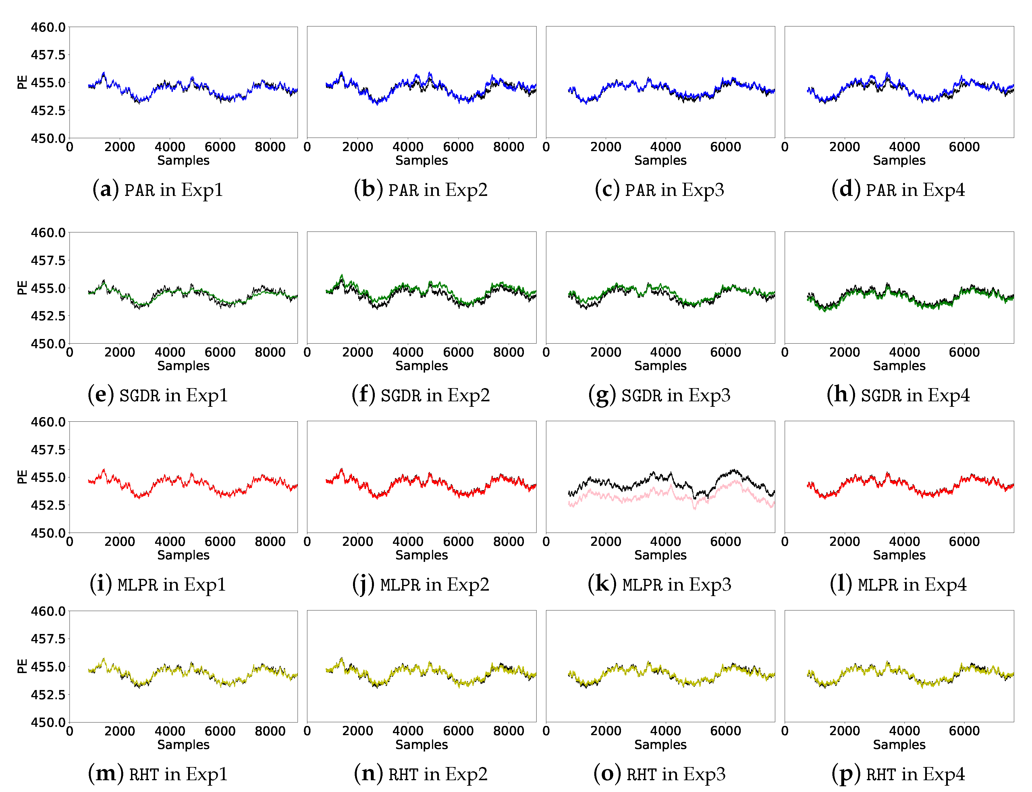
Figure 8 and Figure 9 compiles the real and the predicted values of PE for all SRs in the run 0 of each experiment (of a total of 25 runs), which gives us an overview of the prediction evolution along time.
Finally, Figure 10 depicts the data distribution of ANOVA tests for each experiment (with 25 runs) and SR, which is based on the error metric. The null hypothesis states that the means of all SRs in the experiment are equal, and the alternative hypothesis is that at least one pair is significantly different. The p-values obtained from ANOVA analysis for each experiment (, , , ) are significant (), and therefore, we can conclude that there are significant differences among SRs performances. In order to know how different one SR is from each other, we have performed a Tukey’s range test for each experiment; results suggest that except some cases, all other pairwise comparisons reject null hypothesis and indicate statistical significant differences.
6. Discussion
We start the discussion by highlighting the relevance of having a representative set of preparatory instances in a SL process. As it was introduced in Section 3.2, in streaming scenarios it is not possible to access all historical data, and then it is required to apply some strategy to make assumptions for the incoming data, unless a drift occurs (in which case it would be necessary an adaptation to the new distribution). One of these strategies consists of storing the first instances of the stream (preparatory instances) to carry out a set of preparatory techniques that make the streaming algorithms ready for the streaming process. We have opted for this strategy in our work, and in this section we will explain the impact of these preparatory process on the final performance of the SRs.
Preparatory techniques contribute to improve the performance of the SRs. Theoretically, by selecting a subset of variables/features (variable selection) that contributes most to the prediction variable, we avoid irrelevant or partially relevant features that can negatively impact on the model performance. By selecting the most suitable parameters of algorithms (hyper-parameter tuning), we obtain SRs better adjusted to data. And by training our SRs before the streaming process starts (pre-training), we obtain algorithms ready for the streaming process with better performances. The drawback lies in the fact that as many instances we collect at the beginning of the process, as much time the preparatory techniques will need to be carried out. This is a trade-off that we should have to consider in each scenario, apart from the limits previously mentioned.
Regarding the number of the preparatory instances, as it often occurs with machine learning techniques, the more instances for training (or other purposes) are available, the better the performance of the SRs can be, because data distribution is better represented with more data and the SRs are more trained and adjusted to the data distribution. But on the other hand, the scenario usually poses limits in terms of memory size, computational capacity, or the moment in which the streaming process has to start, among others. Comparing the experiments 1 and 3 (see Table 3 and Table 5 where the selection process was carried out and the preparatory instances were a and of the dataset respectively) with the experiments 2 and 4 (see Table 4 and Table 6 where the variable selection process was not carried out and the preparatory instances were also a and of the dataset respectively), we observe how in almost all cases (except for MTR and MFR when variable selection was carried out) the error metrics improve when the number of preparatory instances is larger. Therefore, by setting aside a group of instances for preparatory purposes, we can generally achieve better results for these stream learners.
In the case of the variable selection process, we deduce from the comparison between Table 3 and Table 4 that this preparatory technique improves the performance of RHT and RHAT, and it also reduces their processing time. For PAR, SGDR, and MLPR, it achieves a similar performance but also reduces their processing time. Thus it is recommendable for all of them, except for MTR and MFR, when the preparatory size is . In the case of the comparison between Table 5 and Table 6, this preparatory technique improves the performances of PAR and RHAT, and it also reduces o maintains their processing time. For SGDR, MLPR and RHT the performances and the processing times are very similar. Thus it is also recommendable for all of them, except again for MTR and MFR, when the preparatory size is . In what refers to which features have been selected for the streaming process in the experiments 1 and 3, we see in Table 7 how AT and V have been preferred over the rest by the hyper-parameter tuning method, which has also been confirmed in Section 5.1 due to their correlation with the target variable (PE).
Regarding the selection of the best SR, Table 3, Table 4, Table 5 and Table 6 show how MLP and RHT show the best error metrics for both preparatory sizes when the variable selection process is carried out. When there is no a variable selection process, then the best error metrics are achieved by MFR. However, in terms of processing time, SGDR and MTR are the fastest stream learners. Due to the fact that we have to find a balance between error metric results and time processing, we recommend RHT. It is worth mentioning that if we check the performance metrics (MSE, RMSE, MAE, and ), RHT shows better results than RHAT, and then we could assume that there are no drift occurrences in the dataset. In case of drifts, RHAT should exhibit better performance metrics than RHT because it has been designed for non-stationary environments.
7. Conclusions
This work has presented a comparison of streaming regressors for electrical power production prediction in a combined cycle power plant. This prediction problem had been tackled before with the traditional thermodynamical analysis, which had shown to be computational and time processing expensive. However, some studies have addressed this problem by applying Machine Learning techniques, such as regression algorithms, and managing to reduce the computational and time costs. These new approaches have considered the problem under a batch learning perspective in which data is assumed to be at rest, and where regression models do not continuously integrate new information into already constructed models. Our work presents a new approach for this scenario, in which data are arriving continuously and where regression models have to learn incrementally. This approach is closer to the emerging Big Data and IoT paradigms.
The results obtained show how competitive error metrics and processing times have been achieved when applying a SL approach to this specific scenario. Specifically, this work has identified RHT as the most recommendable technique to achieve the electrical power production prediction in the CCPP. We have also highlighted the relevance of the preparatory techniques to make the streaming algorithms ready for the streaming process, and at the same time, the importance of selecting properly the number of preparatory instances. Regarding the importance of the features, as in previous cases which tackled the same problem from a batch learning perspective, we do recommend to carry out a variable selection process for all SRs (except for MTR and MFR) because it reduces the streaming processing time and at the same time it is worthy due to the performance gain. Finally, as future work, we would like to transfer this SL approach to other processes in combined cycle power plants, and even to other kinds of electrical power plants.
Author Contributions
Conceptualization, J.L.L., I.B. and I.O.; Methodology, J.L.L. and I.O.; Software, J.L.L. and I.B.; Writing—original draft, J.L.L.; Writing—review & editing, I.B., I.O., J.D.S. and S.S.-S. All authors have read and agreed to the published version of the manuscript.
Funding
This work has been partially supported by the EU project iDev40. This project has received funding from the ECSEL Joint Undertaking (JU) under grant agreement No 783163. The JU receives support from the European Union’s Horizon 2020 research and innovation programme and Austria, Germany, Belgium, Italy, Spain, Romania. It has also been supported by the Basque Government (Spain) through the project VIRTUAL (KK-2018/00096), and by Ministerio de Economía y Competitividad of Spain (Grant Ref. TIN2017-85887-C2-2-P).
Conflicts of Interest
The authors declare no conflict of interest.
Abbreviations
The following abbreviations are used in this manuscript:
| CCPPs | Combined Cycle Power Plants |
| GT | Gas Turbines |
| ST | Steam Turbine |
| SR | Stream Regression |
| IoT | Internet of Things |
| ABB | Asea Brown Boveri |
| AT | Ambient Temperature |
| AP | Atmospheric Pressure |
| RH | Relative Humidity |
| HP | High Pressure |
| LP | Low Pressure |
| D | Drum |
| G | Generator |
| SH | Super Heater |
| E | Evapo |
| V | Vacuum (Exhaust Steam Pressure) |
| EC | Eco |
| HRSG | Heat Recovery Steam Generators |
| PE | Full Load Electrical Power Production |
| PAR | Passive-Aggressive Regressor |
| SGDR | Stochastic Gradient Descent Regressor |
| MLPR | Multi-Layer Perceptron Regressor |
| RHT | Regression Hoeffding Tree |
| RHAT | Regression Hoeffding Adaptive Tree |
| MTR | Mondrian Tree Regressor |
| MFR | Mondrian Forest Regressor |
| ANOVA | ANalysis Of VAriance |
| Exp | Experiment |
| MOA | Massive Online Analysis |
| DDR | Double Data Rate |
| GHz | Giga Hertz |
| MHz | Mega Hertz |
| MAE | Mean Absolute Error |
| RMSE | Root Mean Square Error |
| MSE | Mean Square Error |
| R Squared | |
| ECSEL | Electronic Components and Systems for European Leadership |
| JU | Joint Undertaking |
References
- Black and Veatch. Black and Veatch Strategic Directions: Electric Report; Technical Report; Black and Veatch: Kansas, MO, USA, 2018; Available online: https://www.bv.com/resources/2018-strategic-directionselectric-industry-report (accessed on 28 January 2020).
- Kesgin, U.; Heperkan, H. Simulation of thermodynamic systems using soft computing techniques. Int. J. Energy Res. 2005, 29, 581–611. [Google Scholar] [CrossRef]
- Tüfekci, P. Prediction of full load electrical power output of a base load operated combined cycle power plant using machine learning methods. Int. J. Electr. Power Energy Syst. 2014, 60, 126–140. [Google Scholar] [CrossRef]
- Kaya, H.; Tüfekci, P.; Gürgen, F.S. Local and global learning methods for predicting power of a combined gas & steam turbine. In Proceedings of the International Conference on Emerging Trends in Computer and Electronics Engineering ICETCEE, Dubai, UAE, 24–25 March 2012; pp. 13–18. [Google Scholar]
- Rashid, M.; Kamal, K.; Zafar, T.; Sheikh, Z.; Shah, A.; Mathavan, S. Energy prediction of a combined cycle power plant using a particle swarm optimization trained feedforward neural network. In Proceedings of the 2015 International Conference on Mechanical Engineering, Automation and Control Systems (MEACS), Tomsk, Russia, 1–4 December 2015; pp. 1–5. [Google Scholar]
- Kennedy, J. Particle swarm optimization. Encyclopedia of Machine Learning; John Wiley & Sons: Hoboken, NJ, USA, 2010; pp. 760–766. [Google Scholar]
- Manshad, A.K.; Rostami, H.; Hosseini, S.M.; Rezaei, H. Application of artificial neural network–particle swarm optimization algorithm for prediction of gas condensate dew point pressure and comparison with gaussian processes regression–particle swarm optimization algorithm. J. Energy Resour. Technol. 2016, 138, 032903. [Google Scholar] [CrossRef]
- Cavarzere, A.; Venturini, M. Application of forecasting methodologies to predict gas turbine behavior over time. J. Eng. Gas Turbines Power 2012, 134, 012401. [Google Scholar] [CrossRef]
- Sekhon, R.; Bassily, H.; Wagner, J. A comparison of two trending strategies for gas turbine performance prediction. J. Eng. Gas Turbines Power 2008, 130, 041601. [Google Scholar] [CrossRef]
- Li, Y.; Nilkitsaranont, P. Gas turbine performance prognostic for condition-based maintenance. Appl. Energy 2009, 86, 2152–2161. [Google Scholar] [CrossRef]
- Memon, A.G.; Memon, R.A.; Harijan, K.; Uqaili, M.A. Parametric based thermo-environmental and exergoeconomic analyses of a combined cycle power plant with regression analysis and optimization. Energy Convers. Manag. 2015, 92, 19–35. [Google Scholar] [CrossRef]
- Memon, A.G.; Memon, R.A.; Harijan, K.; Uqaili, M.A. Thermo-environmental analysis of an open cycle gas turbine power plant with regression modeling and optimization. J. Energy Inst. 2014, 87, 81–88. [Google Scholar] [CrossRef]
- Tsoutsanis, E.; Meskin, N. Derivative-driven window-based regression method for gas turbine performance prognostics. Energy 2017, 128, 302–311. [Google Scholar] [CrossRef] [Green Version]
- Tsoutsanis, E.; Meskin, N.; Benammar, M.; Khorasani, K. A dynamic prognosis scheme for flexible operation of gas turbines. Appl. Energy 2016, 164, 686–701. [Google Scholar] [CrossRef] [Green Version]
- Losing, V.; Hammer, B.; Wersing, H. Incremental on-line learning: A review and comparison of state of the art algorithms. Neurocomputing 2018, 275, 1261–1274. [Google Scholar] [CrossRef] [Green Version]
- Khamassi, I.; Sayed-Mouchaweh, M.; Hammami, M.; Ghédira, K. Discussion and review on evolving data streams and concept drift adapting. Evol. Syst. 2018, 9, 1–23. [Google Scholar] [CrossRef]
- Ramírez-Gallego, S.; Krawczyk, B.; García, S.; Woźniak, M.; Herrera, F. A survey on data preprocessing for data stream mining: Current status and future directions. Neurocomputing 2017, 239, 39–57. [Google Scholar] [CrossRef]
- Gomes, H.M.; Barddal, J.P.; Enembreck, F.; Bifet, A. A survey on ensemble learning for data stream classification. ACM Comput. Surv. (CSUR) 2017, 50, 23. [Google Scholar] [CrossRef]
- Tennant, M.; Stahl, F.; Rana, O.; Gomes, J.B. Scalable real-time classification of data streams with concept drift. Future Gener. Comput. Syst. 2017, 75, 187–199. [Google Scholar] [CrossRef]
- Lobo, J.L.; Del Ser, J.; Bilbao, M.N.; Perfecto, C.; Salcedo-Sanz, S. DRED: An evolutionary diversity generation method for concept drift adaptation in online learning environments. Appl. Soft Comput. 2018, 68, 693–709. [Google Scholar] [CrossRef]
- Lobo, J.; Laña, I.; Del, J.S.; Bilbao, M.; Kasabov, N. Evolving Spiking Neural Networks for online learning over drifting data streams. Neural Netw. 2018, 108, 1–19. [Google Scholar] [CrossRef]
- Almeida, P.R.; Oliveira, L.S.; Britto, A.S., Jr.; Sabourin, R. Adapting dynamic classifier selection for concept drift. Expert Syst. Appl. 2018, 104, 67–85. [Google Scholar] [CrossRef]
- De Barros, R.S.M.; de Carvalho Santos, S.G.T. An Overview and Comprehensive Comparison of Ensembles for Concept Drift. Inf. Fusion 2019, 52, 213–244. [Google Scholar] [CrossRef]
- Benczúr, A.A.; Kocsis, L.; Pálovics, R. Online Machine Learning in Big Data Streams. arXiv 2018, arXiv:1802.05872. [Google Scholar]
- Krawczyk, B.; Minku, L.L.; Gama, J.; Stefanowski, J.; Woźniak, M. Ensemble learning for data stream analysis: A survey. Inf. Fusion 2017, 37, 132–156. [Google Scholar] [CrossRef]
- Lughofer, E.; Pratama, M. Online active learning in data stream regression using uncertainty sampling based on evolving generalized fuzzy models. IEEE Trans. Fuzzy Syst. 2017, 26, 292–309. [Google Scholar] [CrossRef]
- Ikonomovska, E.; Gama, J.; Džeroski, S. Online tree-based ensembles and option trees for regression on evolving data streams. Neurocomputing 2015, 150, 458–470. [Google Scholar] [CrossRef] [Green Version]
- Zhou, Z.H.; Chawla, N.V.; Jin, Y.; Williams, G.J. Big data opportunities and challenges: Discussions from data analytics perspectives [discussion forum]. IEEE Comput. Intell. Mag. 2014, 9, 62–74. [Google Scholar] [CrossRef] [Green Version]
- Chen, M.; Mao, S.; Liu, Y. Big data: A survey. Mob. Netw. Appl. 2014, 19, 171–209. [Google Scholar] [CrossRef]
- Domingos, P.; Hulten, G. A general framework for mining massive data streams. J. Comput. Graph. Stat. 2003, 12, 945–949. [Google Scholar] [CrossRef]
- Lu, J.; Liu, A.; Dong, F.; Gu, F.; Gama, J.; Zhang, G. Learning under Concept Drift: A Review. IEEE Trans. Knowl. Data Eng. 2018, 31, 2346–2363. [Google Scholar] [CrossRef] [Green Version]
- Alippi, C. Intelligence for Embedded Systems; Springer: Heidelberg, Germany, 2014. [Google Scholar]
- Žliobaitė, I.; Pechenizkiy, M.; Gama, J. An overview of concept drift applications. In Big Data Analysis: New Algorithms for a New Society; Springer: Heidelberg, Germany, 2016; pp. 91–114. [Google Scholar]
- De Francisci Morales, G.; Bifet, A.; Khan, L.; Gama, J.; Fan, W. Iot big data stream mining. In Proceedings of the 22nd ACM SIGKDD International Conference on Knowledge Discovery and Data Mining, San Francisco, CA, USA, 13–17 August 2016; pp. 2119–2120. [Google Scholar]
- Manyika, J.; Chui, M.; Bisson, P.; Woetzel, J.; Dobbs, R.; Bughin, J.; Aharon, D. Unlocking the potential of the Internet of Things; McKinsey Global Institute: Kerala, India, 2015. [Google Scholar]
- Mahmud, R.; Kotagiri, R.; Buyya, R. Fog computing: A taxonomy, survey and future directions. In Internet of Everything; Springer: Heidelberg, Germany, 2018; pp. 103–130. [Google Scholar]
- Tang, B.; Chen, Z.; Hefferman, G.; Pei, S.; Wei, T.; He, H.; Yang, Q. Incorporating intelligence in fog computing for big data analysis in smart cities. IEEE Trans. Ind. Inform. 2017, 13, 2140–2150. [Google Scholar] [CrossRef]
- Mohammadi, M.; Al-Fuqaha, A.; Sorour, S.; Guizani, M. Deep learning for IoT big data and streaming analytics: A survey. IEEE Commun. Surv. Tutor. 2018, 20, 2923–2960. [Google Scholar] [CrossRef] [Green Version]
- Lasi, H.; Fettke, P.; Kemper, H.G.; Feld, T.; Hoffmann, M. Industry 4.0. Bus. Inf. Syst. Eng. 2014, 6, 239–242. [Google Scholar] [CrossRef]
- Niu, L.; Liu, X. Multivariable generalized predictive scheme for gas turbine control in combined cycle power plant. In Proceedings of the 2008 IEEE Conference on Cybernetics and Intelligent Systems, Chengdu, China, 21–24 September 2008; pp. 791–796. [Google Scholar]
- Ramireddy, V. An Overview of Combined Cycle Power Plant. Electrical Engineering, 25 August 2012. [Google Scholar]
- Chen, Z.; Liu, B. Lifelong machine learning. Synth. Lect. Artif. Intell. Mach. Learn. 2016, 10, 1–145. [Google Scholar] [CrossRef] [Green Version]
- Gama, J.; Žliobaitė, I.; Bifet, A.; Pechenizkiy, M.; Bouchachia, A. A survey on concept drift adaptation. ACM Comput. Surv. (CSUR) 2014, 46, 1–37. [Google Scholar] [CrossRef]
- Draper, N.R.; Smith, H. Applied Regression Analysis; John Wiley & Sons: Hoboken, NJ, USA, 2014; Volume 326. [Google Scholar]
- Montiel, J.; Read, J.; Bifet, A.; Abdessalem, T. Scikit-multiflow: A multi-output streaming framework. J. Mach. Learn. Res. 2018, 19, 2914–2915. [Google Scholar]
- Pedregosa, F.; Varoquaux, G.; Gramfort, A.; Michel, V.; Thirion, B.; Grisel, O.; Blondel, M.; Prettenhofer, P.; Weiss, R.; Dubourg, V.; et al. Scikit-learn: Machine learning in Python. J. Mach. Learn. Res. 2011, 12, 2825–2830. [Google Scholar]
- Crammer, K.; Dekel, O.; Keshet, J.; Shalev-Shwartz, S.; Singer, Y. Online passive-aggressive algorithms. J. Mach. Learn. Res. 2006, 7, 551–585. [Google Scholar]
- Bottou, L. Large-scale machine learning with stochastic gradient descent. In Proceedings of COMPSTAT’2010; Springer: Heidelberg, Germany, 2010; pp. 177–186. [Google Scholar]
- Zhang, T. Solving large scale linear prediction problems using stochastic gradient descent algorithms. In Proceedings of the Twenty-First International Conference on Machine Learning, Banff, AB, Canada, 4–8 July 2004; p. 116. [Google Scholar]
- Rumelhart, D.E.; Hinton, G.E.; Williams, R.J. Learning representations by back-propagating errors. Nature 1986, 323, 533–536. [Google Scholar] [CrossRef]
- Domingos, P.; Hulten, G. Mining high-speed data streams. In Proceedings of the Sixth ACM SIGKDD International Conference on Knowledge Discovery and Data, Boston, MA, USA, 20–23 August 2000; Volume 2, p. 4. [Google Scholar]
- Ikonomovska, E.; Gama, J.; Džeroski, S. Learning model trees from evolving data streams. Data Min. Knowl. Discov. 2011, 23, 128–168. [Google Scholar] [CrossRef] [Green Version]
- Bifet, A.; Gavalda, R. Learning from time-changing data with adaptive windowing. In Proceedings of the 2007 SIAM International Conference on Data Mining, Minneapolis, MN, USA, 26–28 April 2007; pp. 443–448. [Google Scholar]
- Lakshminarayanan, B.; Roy, D.M.; Teh, Y.W. Mondrian forests. In Advances in Neural Information Processing Systems; MIT Press: Cambridge, MA, USA, 2014; pp. 3140–3148. [Google Scholar]
- Oliphant, T.E. Python for scientific computing. Comput. Sci. Eng. 2007, 9, 10–20. [Google Scholar] [CrossRef] [Green Version]
- Bifet, A.; Gavaldà, R.; Holmes, G.; Pfahringer, B. Machine Learning for Data Streams with Practical Examples in MOA; MIT Press: Cambridge, MA, USA, 2018. [Google Scholar]
- Benesty, J.; Chen, J.; Huang, Y.; Cohen, I. Pearson correlation coefficient. In Noise Reduction in Speech Processing; Springer: Heidelberg, Germany, 2009; pp. 1–4. [Google Scholar]
- Bifet, A.; de Francisci Morales, G.; Read, J.; Holmes, G.; Pfahringer, B. Efficient online evaluation of big data stream classifiers. In Proceedings of the 21th ACM SIGKDD International Conference on Knowledge Discovery and Data Mining, Sydney, Australia, 10–13 August 2015; pp. 59–68. [Google Scholar]
- Scheffe, H. The Analysis of Variance; John Wiley & Sons: Hoboken, NJ, USA, 1999; Volume 72. [Google Scholar]
- Alpaydin, E. Introduction to Machine Learning; MIT Press: Cambridge, MA, USA, 2009. [Google Scholar]
- Tukey, J.W. Comparing individual means in the analysis of variance. Biometrics 1949, 5, 99–114. [Google Scholar] [CrossRef]
- Arrieta, F.R.P.; Lora, E.E.S. Influence of ambient temperature on combined-cycle power-plant performance. Appl. Energy 2005, 80, 261–272. [Google Scholar] [CrossRef]
- De Sa, A.; Al Zubaidy, S. Gas turbine performance at varying ambient temperature. Appl. Therm. Eng. 2011, 31, 2735–2739. [Google Scholar] [CrossRef]
- Erdem, H.H.; Sevilgen, S.H. Case study: Effect of ambient temperature on the electricity production and fuel consumption of a simple cycle gas turbine in Turkey. Appl. Therm. Eng. 2006, 26, 320–326. [Google Scholar] [CrossRef]
- Patel, M.; Nath, N. Improve Steam Turbine Efficiency. Hydrocarb. Process. 2000, 79, 85–90. [Google Scholar]
- Lee, J.J.; Kim, T.S.; Kim, T.S. Development of a gas turbine performance analysis program and its application. Energy 2011, 36, 5274–5285. [Google Scholar] [CrossRef]
Figure 1.
Layout of the combined cycle power plant based on [3]. HP is High Pressure, LP is Low Pressure, D is Drum, G is Generator, SH is Super Heater, E is Evapo, EC is Eco, and HRSG is Heat Recovery Steam Generators. AT, AP, RH, V and PE are the variables described in Table 1.

Figure 2.
Scheme of the SL process of this work.

Figure 3.
Stream learning (online learning) scheme with test-then-train evaluation.

Figure 4.
Traditional scheme when evaluating a non-incremental algorithm in batch processing mode.

Figure 5.
Training and testing of an incremental algorithm in batch processing mode. Note that only the last model is used for prediction.
Figure 5.
Training and testing of an incremental algorithm in batch processing mode. Note that only the last model is used for prediction.

Figure 6.
Scatter diagram for visualizing the correlation between features, and the linear regression model fit to the data.
Figure 6.
Scatter diagram for visualizing the correlation between features, and the linear regression model fit to the data.

Figure 7.
Heat map for visualizing the correlation between features.

Figure 8.
Real (black line) and predicted (colored line) PEs of PAR, SGDR, MLPR and RHT for run 0. A moving average of 750 instances (1 month approx.) has been applied to smooth out short-term fluctuations.
Figure 8.
Real (black line) and predicted (colored line) PEs of PAR, SGDR, MLPR and RHT for run 0. A moving average of 750 instances (1 month approx.) has been applied to smooth out short-term fluctuations.

Figure 9.
Real (black line) and predicted (colored line) PEs of RHAT, MFR and MTR for run 0. A moving average of 750 instances (1 month approx.) has been applied to smooth out short-term fluctuations.
Figure 9.
Real (black line) and predicted (colored line) PEs of RHAT, MFR and MTR for run 0. A moving average of 750 instances (1 month approx.) has been applied to smooth out short-term fluctuations.

Figure 10.
Boxplots of ANOVA tests for in each experiment.


Table 1.
Input and target variables of the dataset.
| Variables | Descriptions | Ranges | Types |
|---|---|---|---|
| Ambient Temperature | Measured in whole degrees in Celsius | Input | |
| Atmospheric Pressure | Measured in units of milibars | Input | |
| Relative Humidity | Measured as a percentage | Input | |
| Vacuum (Exhaust Steam Pressure) | Measured in cm Hg | Input | |
| Full Load Electrical Power Production | Measured in megawatts | Target |
Table 2.
The experimental benchmark for the comparison of the SRs.
| Preparatory Sizes (% of the Dataset) | |||
|---|---|---|---|
| Variable selection | True | Exp1 | Exp3 |
| False | Exp2 | Exp4 | |
Table 3.
Results of the experiment 1: variable selection with a of preparatory instances. Note that RMSE=MAE because all differences are equal.
Table 3.
Results of the experiment 1: variable selection with a of preparatory instances. Note that RMSE=MAE because all differences are equal.
| SR | MSE | RMSE | MAE | TIME (s) | |
|---|---|---|---|---|---|
| PAR | 0.007 ± 0.011 | 0.062 ± 0.049 | 0.062 ± 0.049 | 0.872 ± 0.070 | 2.97 ± 0.71 |
| SGDR | 0.008 ± 0.013 | 0.070 ± 0.056 | 0.070 ± 0.056 | 0.829 ± 0.123 | 2.31 ± 0.38 |
| MLPR | 0.005 ± 0.007 | 0.055 ± 0.041 | 0.055 ± 0.041 | 0.901 ± 0.011 | 9.23 ± 7.78 |
| RHT | 0.004 ± 0.006 | 0.052 ± 0.039 | 0.052 ± 0.039 | 0.900 ± 0.024 | 2.55 ± 0.55 |
| RHAT | 0.005 ± 0.007 | 0.054 ± 0.040 | 0.054 ± 0.040 | 0.893 ± 0.024 | 3.87 ± 0.75 |
| MFR | 0.021 ± 0.029 | 0.109 ± 0.091 | 0.109 ± 0.091 | 0.592 ± 0.203 | 107.06 ± 49.95 |
| MTR | 0.019 ± 0.027 | 0.104 ± 0.086 | 0.104 ± 0.086 | 0.629 ± 0.186 | 1.344 ± 0.18 |
Table 4.
Results of the experiment 2: no variable selection with a of preparatory instances. Note that RMSE=MAE because all differences are equal.
Table 4.
Results of the experiment 2: no variable selection with a of preparatory instances. Note that RMSE=MAE because all differences are equal.
| SR | MSE | RMSE | MAE | TIME (s) | |
|---|---|---|---|---|---|
| PAR | 0.006 ± 0.009 | 0.057 ± 0.044 | 0.057 ± 0.044 | 0.885 ± 0.013 | 3.29 ± 1.50 |
| SGDR | 0.008 ± 0.012 | 0.069 ± 0.053 | 0.069 ± 0.053 | 0.821 ± 0.119 | 2.48 ± 0.90 |
| MLPR | 0.005 ± 0.007 | 0.055 ± 0.041 | 0.055 ± 0.041 | 0.897 ± 0.020 | 14.76 ± 12.51 |
| RHT | 0.005 ± 0.007 | 0.052 ± 0.040 | 0.052 ± 0.040 | 0.876 ± 0.047 | 3.55 ± 0.70 |
| RHAT | 0.005 ± 0.007 | 0.054 ± 0.04 | 0.054 ± 0.040 | 0.884 ± 0.038 | 5.42 ± 0.94 |
| MFR | 0.004 ± 0.007 | 0.042 ± 0.039 | 0.042 ± 0.039 | 0.922 ± 0.041 | 125.18 ± 60.71 |
| MTR | 0.012 ± 0.021 | 0.076 ± 0.073 | 0.076 ± 0.073 | 0.754 ± 0.171 | 1.49 ± 0.23 |
Table 5.
Results of the experiment 3: variable selection with a of preparatory instances. Note that RMSE=MAE because all differences are equal.
Table 5.
Results of the experiment 3: variable selection with a of preparatory instances. Note that RMSE=MAE because all differences are equal.
| SR | MSE | RMSE | MAE | TIME (s) | |
|---|---|---|---|---|---|
| PAR | 0.005 ± 0.007 | 0.055 ± 0.041 | 0.055 ± 0.041 | 0.904 ± 0.013 | 2.40 ± 0.90 |
| SGDR | 0.005 ± 0.007 | 0.056 ± 0.041 | 0.056 ± 0.041 | 0.901 ± 0.021 | 1.86 ± 0.58 |
| MLPR | 0.004 ± 0.007 | 0.052 ± 0.039 | 0.052 ± 0.039 | 0.912 ± 0.016 | 9.12 ± 8.83 |
| RHT | 0.004 ± 0.006 | 0.050 ± 0.037 | 0.050 ± 0.037 | 0.914 ± 0.010 | 2.07 ± 0.28 |
| RHAT | 0.004 ± 0.007 | 0.052 ± 0.039 | 0.052 ± 0.039 | 0.909 ± 0.010 | 3.48 ± 0.57 |
| MFR | 0.022 ± 0.030 | 0.113 ± 0.092 | 0.113 ± 0.092 | 0.570 ± 0.205 | 94.98 ± 42.94 |
| MTR | 0.024 ± 0.031 | 0.120 ± 0.093 | 0.120 ± 0.093 | 0.539 ± 0.178 | 1.11 ± 0.16 |
Table 6.
Results of the experiment 4: no variable selection with a of preparatory instances. Note that RMSE=MAE because all differences are equal.
Table 6.
Results of the experiment 4: no variable selection with a of preparatory instances. Note that RMSE=MAE because all differences are equal.
| SR | MSE | RMSE | MAE | TIME (s) | |
|---|---|---|---|---|---|
| PAR | 0.006 ± 0.010 | 0.057 ± 0.044 | 0.057 ± 0.044 | 0.890 ± 0.010 | 2.38 ± 0.79 |
| SGDR | 0.005 ± 0.007 | 0.055 ± 0.040 | 0.055 ± 0.040 | 0.901 ± 0.014 | 1.79 ± 0.48 |
| MLPR | 0.004 ± 0.006 | 0.051 ± 0.037 | 0.051 ± 0.037 | 0.917 ± 0.011 | 7.96 ± 7.12 |
| RHT | 0.004 ± 0.006 | 0.048 ± 0.036 | 0.048 ± 0.036 | 0.917 ± 0.023 | 3.12 ± 0.43 |
| RHAT | 0.005 ± 0.007 | 0.055 ± 0.041 | 0.055 ± 0.041 | 0.892 ± 0.039 | 5.16 ± 1.18 |
| MFR | 0.003 ± 0.006 | 0.036 ± 0.035 | 0.036 ± 0.035 | 0.940 ± 0.053 | 109.65 ± 42.04 |
| MTR | 0.011 ± 0.019 | 0.075 ± 0.070 | 0.075 ± 0.070 | 0.776 ± 0.126 | 1.21 ± 0.21 |
Table 7.
Variable selection results in each experiment. Those selected features are represented with y (yes), the rest with n (no).
Table 7.
Variable selection results in each experiment. Those selected features are represented with y (yes), the rest with n (no).
| Features | |||||
|---|---|---|---|---|---|
| AT | AP | RH | V | ||
| Experiments | 1 | y | n | n | y |
| 3 | y | n | n | y | |
Table 8.
Hyper-parameter tuning results for SRs in the experiment 1.
| SR | Parameters | Values |
|---|---|---|
| PAR | C | 0.05 |
| SGDR | alpha | 0.1/0.01 |
| loss | epsilon_insensitive | |
| penalty | L1/L2 | |
| learning_rate | constant/optimal | |
| MLPR | hidden_layer_sizes | (50,50) |
| activation | relu | |
| solver | adam/sgd | |
| learning_rate | constant, invscaling, adaptive | |
| learning_rate_init | 0.005/0.001 | |
| alpha | 0.000001-0.000000001 | |
| RHT | grace_period | 200 |
| split_confidence | 0.0000001 | |
| tie_threshold | 0.05 | |
| leaf_prediction | perceptron | |
| RHAT | grace_period | 200 |
| split_confidence | 0.0000001 | |
| tie_threshold | 0.05 | |
| leaf_prediction | perceptron | |
| delta (ADWIN detector) | 0.002 | |
| MTR | max_depth | 10–100 |
| min_samples_split | 10 | |
| MFR | max_depth | 10–80 |
| min_samples_split | 10 | |
| n_estimators | 50/100 |
Table 9.
Hyper-parameter tuning results for SRs in the experiment 2.
| SR | Parameters | Values |
|---|---|---|
| PAR | C | 0.5/1.0 |
| SGDR | alpha | 0.00001–0.1 |
| loss | epsilon_insensitive | |
| penalty | L1/L2 | |
| learning_rate | constant/optimal/invscaling | |
| MLPR | hidden_layer_sizes | (50,50)/(100,100) |
| activation | relu/tanh/identity | |
| solver | adam/sgd | |
| learning_rate | constant, invscaling, adaptive | |
| learning_rate_init | 0.0005-0.05 | |
| alpha | 0.00001-0.000000001 | |
| RHT | grace_period | 200 |
| split_confidence | 0.0000001 | |
| tie_threshold | 0.05 | |
| leaf_prediction | perceptron | |
| RHAT | grace_period | 200 |
| split_confidence | 0.0000001 | |
| tie_threshold | 0.05 | |
| leaf_prediction | perceptron | |
| delta (ADWIN detector) | 0.002 | |
| MTR | max_depth | 20–90 |
| min_samples_split | 2/5/10 | |
| MFR | max_depth | 20–90 |
| min_samples_split | 2/5 | |
| n_estimators | 50/100 |
Table 10.
Hyper-parameter tuning results for SRs in the experiment 3.
| SR | Parameters | Values |
|---|---|---|
| PAR | C | 0.01 |
| SGDR | alpha | |
| loss | epsilon_insensitive | |
| penalty | elasticnet/L1 | |
| learning_rate | constant | |
| MLPR | hidden_layer_sizes | |
| activation | relu | |
| solver | adam/sgd | |
| learning_rate | constant, invscaling, adaptive | |
| learning_rate_init | ||
| alpha | ||
| RHT | grace_period | 200 |
| split_confidence | ||
| tie_threshold | ||
| leaf_prediction | perceptron | |
| RHAT | grace_period | 200 |
| split_confidence | ||
| tie_threshold | ||
| leaf_prediction | perceptron | |
| delta (ADWIN detector) | ||
| MTR | max_depth | 20–60 |
| min_samples_split | 10 | |
| MFR | max_depth | 20–60 |
| min_samples_split | 10 | |
| n_estimators |
Table 11.
Hyper-parameter tuning results for SRs in the experiment 4.
| SR | Parameters | Values |
|---|---|---|
| PAR | C | |
| SGDR | alpha | 0.001–0.01 |
| loss | epsilon_insensitive | |
| penalty | L1/L2 | |
| learning_rate | constant/optimal | |
| MLPR | hidden_layer_sizes | |
| activation | relu/tanh | |
| solver | adam/sgd | |
| learning_rate | constant, invscaling, adaptive | |
| learning_rate_init | 0.0005–0.05 | |
| alpha | 0.001–0.000000001 | |
| RHT | grace_period | 200 |
| split_confidence | ||
| tie_threshold | ||
| leaf_prediction | perceptron | |
| RHAT | grace_period | 200 |
| split_confidence | ||
| tie_threshold | ||
| leaf_prediction | perceptron | |
| delta (ADWIN detector) | 0.002 | |
| MTR | max_depth | 40–100 |
| min_samples_split | 5 | |
| MFR | max_depth | 30–100 |
| min_samples_split | 5 | |
| n_estimators |
Table 12.
Results of the Tukey’s range test for experiment 1.
| Group1 | Group2 | MEAN DIFF. | Lower | Upper | Reject |
|---|---|---|---|---|---|
| MFR | MLPR | 0.259 | 0.1317 | 0.3864 | True |
| MFR | MTR | −0.0108 | −0.1382 | 0.1165 | False |
| MFR | PAR | 0.2375 | 0.1102 | 0.3649 | True |
| MFR | RHAT | 0.2461 | 0.1188 | 0.3735 | True |
| MFR | RHT | 0.2546 | 0.1272 | 0.3819 | True |
| MFR | SGDR | 0.2037 | 0.0764 | 0.3311 | True |
| MLPR | MTR | −0.2699 | −0.3972 | −0.1425 | True |
| MLPR | PAR | −0.0215 | −0.1489 | 0.1058 | False |
| MLPR | RHAT | −0.0129 | −0.1403 | 0.1144 | False |
| MLPR | RHT | −0.0045 | −0.1318 | 0.1229 | False |
| MLPR | SGDR | −0.0553 | −0.1827 | 0.072 | False |
| MTR | PAR | 0.2484 | 0.121 | 0.3757 | True |
| MTR | RHAT | 0.257 | 0.1296 | 0.3843 | True |
| MTR | RHT | 0.2654 | 0.138 | 0.3928 | True |
| MTR | SGDR | 0.2146 | 0.0872 | 0.3419 | True |
| PAR | RHAT | 0.0086 | −0.1188 | 0.1359 | False |
| PAR | RHT | 0.017 | −0.1103 | 0.1444 | False |
| PAR | SGDR | −0.0338 | −0.1612 | 0.0936 | False |
| RHAT | RHT | 0.0084 | −0.1189 | 0.1358 | False |
| RHAT | SGDR | −0.0424 | −0.1697 | 0.085 | False |
| RHT | SGDR | −0.0508 | −0.1782 | 0.0765 | False |
Table 13.
Results of the Tukey’s range test for experiment 2.
| Group1 | Group2 | Mean Diff. | Lower | Upper | Reject |
|---|---|---|---|---|---|
| MFR | MLPR | −0.0223 | −0.1304 | 0.0859 | False |
| MFR | MTR | −0.1953 | −0.3035 | −0.0871 | True |
| MFR | PAR | −0.0381 | −0.1463 | 0.07 | False |
| MFR | RHAT | −0.0428 | −0.151 | 0.0653 | False |
| MFR | RHT | −0.0259 | −0.1341 | 0.0823 | False |
| MFR | SGDR | −0.1408 | −0.249 | −0.0326 | True |
| MLPR | MTR | −0.173 | −0.2812 | −0.0649 | True |
| MLPR | PAR | −0.0159 | −0.1241 | 0.0923 | False |
| MLPR | RHAT | −0.0206 | −0.1287 | 0.0876 | False |
| MLPR | RHT | −0.0036 | −0.1118 | 0.1045 | False |
| MLPR | SGDR | −0.1185 | −0.2267 | −0.0103 | True |
| MTR | PAR | 0.1572 | 0.049 | 0.2653 | True |
| MTR | RHAT | 0.1525 | 0.0443 | 0.2606 | True |
| MTR | RHT | 0.1694 | 0.0612 | 0.2776 | True |
| MTR | SGDR | 0.0545 | −0.0537 | 0.1627 | False |
| PAR | RHAT | −0.0047 | −0.1129 | 0.1035 | False |
| PAR | RHT | 0.0122 | −0.0959 | 0.1204 | False |
| PAR | SGDR | −0.1026 | −0.2108 | 0.0055 | False |
| RHAT | RHT | 0.0169 | −0.0913 | 0.1251 | False |
| RHAT | SGDR | −0.0979 | −0.2061 | 0.0102 | False |
| RHT | SGDR | −0.1149 | −0.223 | −0.0067 | True |
Table 14.
Results of the Tukey’s range test for experiment 3.
| Group1 | Group2 | Mean Diff. | Lower | Upper | Reject |
|---|---|---|---|---|---|
| MFR | MLPR | 0.2913 | 0.1947 | 0.3879 | True |
| MFR | MTR | −0.0508 | −0.1474 | 0.0458 | False |
| MFR | PAR | 0.2892 | 0.1926 | 0.3859 | True |
| MFR | RHAT | 0.2955 | 0.1988 | 0.3921 | True |
| MFR | RHT | 0.293 | 0.1963 | 0.3896 | True |
| MFR | SGDR | 0.2874 | 0.1908 | 0.3841 | True |
| MLPR | MTR | −0.3421 | −0.4387 | −0.2455 | True |
| MLPR | PAR | −0.0021 | −0.0987 | 0.0945 | False |
| MLPR | RHAT | 0.0042 | −0.0925 | 0.1008 | False |
| MLPR | RHT | 0.0016 | −0.095 | 0.0983 | False |
| MLPR | SGDR | −0.0039 | −0.1005 | 0.0927 | False |
| MTR | PAR | 0.34 | 0.2434 | 0.4367 | True |
| MTR | RHAT | 0.3463 | 0.2496 | 0.4429 | True |
| MTR | RHT | 0.3438 | 0.2471 | 0.4404 | True |
| MTR | SGDR | 0.3382 | 0.2416 | 0.4348 | True |
| PAR | RHAT | 0.0062 | −0.0904 | 0.1029 | False |
| PAR | RHT | 0.0037 | −0.0929 | 0.1004 | False |
| PAR | SGDR | −0.0018 | −0.0984 | 0.0948 | False |
| RHAT | RHT | −0.0025 | −0.0991 | 0.0941 | False |
| RHAT | SGDR | −0.0081 | −0.1047 | 0.0886 | False |
| RHT | SGDR | −0.0055 | −0.1022 | 0.0911 | False |
Table 15.
Results of the Tukey’s range test for experiment 4.
| Group1 | Group2 | Mean Diff. | Lower | Upper | Reject |
|---|---|---|---|---|---|
| MFR | MLPR | −0.0352 | −0.1058 | 0.0355 | False |
| MFR | MTR | −0.2079 | −0.2786 | −0.1372 | True |
| MFR | PAR | −0.0549 | −0.1255 | 0.0158 | False |
| MFR | RHAT | −0.0494 | −0.1201 | 0.0212 | False |
| MFR | RHT | −0.0307 | −0.1013 | 0.04 | False |
| MFR | SGDR | −0.0604 | −0.131 | 0.0103 | False |
| MLPR | MTR | −0.1727 | −0.2434 | −0.1021 | True |
| MLPR | PAR | −0.0197 | −0.0904 | 0.051 | False |
| MLPR | RHAT | −0.0143 | −0.0849 | 0.0564 | False |
| MLPR | RHT | 0.0045 | −0.0662 | 0.0752 | False |
| MLPR | SGDR | −0.0252 | −0.0959 | 0.0455 | False |
| MTR | PAR | 0.153 | 0.0824 | 0.2237 | True |
| MTR | RHAT | 0.1585 | 0.0878 | 0.2291 | True |
| MTR | RHT | 0.1772 | 0.1066 | 0.2479 | True |
| MTR | SGDR | 0.1475 | 0.0769 | 0.2182 | True |
| PAR | RHAT | 0.0054 | −0.0652 | 0.0761 | False |
| PAR | RHT | 0.0242 | −0.0465 | 0.0949 | False |
| PAR | SGDR | −0.0055 | −0.0762 | 0.0652 | False |
| RHAT | RHT | 0.0188 | −0.0519 | 0.0894 | False |
| RHAT | SGDR | −0.0109 | −0.0816 | 0.0597 | False |
| RHT | SGDR | −0.0297 | −0.1004 | 0.0409 | False |
© 2020 by the authors. Licensee MDPI, Basel, Switzerland. This article is an open access article distributed under the terms and conditions of the Creative Commons Attribution (CC BY) license (http://creativecommons.org/licenses/by/4.0/).
Share and Cite
MDPI and ACS Style
Lobo, J.L.; Ballesteros, I.; Oregi, I.; Del Ser, J.; Salcedo-Sanz, S. Stream Learning in Energy IoT Systems: A Case Study in Combined Cycle Power Plants. Energies 2020, 13, 740. https://doi.org/10.3390/en13030740
AMA Style
Lobo JL, Ballesteros I, Oregi I, Del Ser J, Salcedo-Sanz S. Stream Learning in Energy IoT Systems: A Case Study in Combined Cycle Power Plants. Energies. 2020; 13(3):740. https://doi.org/10.3390/en13030740
Chicago/Turabian StyleLobo, Jesus L., Igor Ballesteros, Izaskun Oregi, Javier Del Ser, and Sancho Salcedo-Sanz. 2020. "Stream Learning in Energy IoT Systems: A Case Study in Combined Cycle Power Plants" Energies 13, no. 3: 740. https://doi.org/10.3390/en13030740
Note that from the first issue of 2016, this journal uses article numbers instead of page numbers. See further details here.