A Numerical Study on the Characteristics of Air–Fuel Mixing Using a Fluidic Oscillator in Supersonic Flow Fields

Department of Aerospace Engineering, Inha University, Incheon 22212, Korea
*
Author to whom correspondence should be addressed.
Energies 2019, 12(24), 4758; https://doi.org/10.3390/en12244758
Submission received: 19 November 2019
/
Revised: 4 December 2019
/
Accepted: 10 December 2019
/
Published: 13 December 2019
Abstract
:In this study, numerical simulations were conducted to confirm the possibility of improved mixing performance by using a fluidic oscillator as a fuel injector. Three-dimensional URANS non-reacting simulations were conducted to examine air–fuel mixing in a supersonic flow field of Mach 3.38. The numerical methods were validated through simulations of the oscillating flow generated from the fluidic oscillator. The results show that the mass flow rate and momentum are reduced at the outlet because the total pressure loss increases inside the fluidic oscillator, which means that higher pressure needs to be applied to supply the same mass flow rate. The simulation showed that the flow structure varies over time as the injected flow is swept laterally. With lateral injection, the fuel distribution is long and narrow, and asymmetric vortexes are generated. However, with central injection, the fuel distribution is relatively similar to the case of using a simple injector. Compared to the simple injector, the penetration length, flammable area, and mixing efficiency were improved. However, the total pressure loss in the flow field increases as well. The results showed that the supersonic fluidic oscillator could be fully utilized as a means to enhance the mixing effect, however a method to reduce the total pressure loss is necessary for practical application.
1. Introduction
A scramjet engine is a next-generation engine that can be operated in the hypersonic regime. Many studies have been conducted since the concept of supersonic combustion was presented by Ferri [1], but scramjets have not yet been developed to the stage of practical application due to technical difficulties. One of the main difficulties is related to the proper mixing of the air–fuel. The air from the intake flows at supersonic speed, so the fuel and air have a very short residence time in the combustion chamber. To overcome this issue, many studies have been conducted on more efficient and faster air–fuel mixing techniques, which are largely divided into passive and active methods [2].
Passive methods use a specific structure inside the combustion chamber or change the configuration of the wall to form a vortex and recirculation zone in the flow, which result in improved air–fuel mixing performance for higher combustion performance. Various methods have been studied, such as pylons [3,4,5,6], cavities [7,8,9,10,11,12,13,14], hyper-mixers [15,16,17,18,19,20,21], injector locations [22], angles [23,24], and outlet shapes [25]. A pylon is a slim structure on the wall of the combustion chamber that generates a recirculation zone and vortex to promote air–fuel mixing and stabilize the flame. Studies have been conducted on the mixing efficiency and flow characteristics according to the shape of the pylon [3,4,5] and to derive an optimal shape [6].
It is relatively easy to improve the mixing efficiency, but there is a disadvantage of significantly increasing the total pressure loss at a high Mach number. The cavity has been studied because it helps to mix the air–fuel and it can more effectively hold the flame in empty space where a recirculation zone can be formed on the wall [7,8,9,10,11,12,13,14]. A number of studies have been conducted on experiments or numerical simulations to observe the interaction of the cavity with flow fields in the combustion chamber [13] and derive the optimum cavity shape [7,8,9]. Recent studies have been conducted to find ways to improve the mixing performance through more diverse attempts, such as variable cavities and pylons and double cavities [10,11,14].
Using the cavity, a scramjet engine can efficiently mix the air–fuel and hold the flame more easily with less total pressure loss. However, combustion instability can occur due to acoustic interference, and additional systems may be needed to compensate for this. A hyper-mixer is a system where a part of the wall of a combustion chamber has a form such as a ramp or a step. The shape generally induces a counter-rotating vortex, which helps to improve the mixing efficiency and expansion of the mixed area [15,16,17,18,19,20,21]. Studies have been carried out on adjusting the angle, arrangement, and shape of the injector [23,24,25] and using a swirler or counterflow nozzle [26,27].
Unlike passive methods, active methods actively intervene in the flow of combustion chambers. Pulsed injection [28,29,30,31,32,33] and the Hartmann–Sprenger (H-S) tube [34,35] are examples of ways to directly affect the flow through various control methods. In pulsed injection, the flow field is changed by repeated injection and shutdown of the fuel at regular intervals. Pulsed injection flow-through devices such as orifices and valves have been studied, and the unsteady flow and mixing characteristics have been reported [28,29,30,31,32,33]. The results showed that the unsteady flow field near the injector improves the penetration length and mixing performance. However, the disadvantage is that the mass flow rate of the injection gas is lower than in continuous injection under the same total pressure conditions of the injector inlet. Increasing the pressure at the inlet to overcome this causes another problem: over-expanding of the flow at the injector outlet.
An H-S tube is an acoustic device that produces high-frequency sound and is used in flow excitation. Parametric studies have observed the effects of the shape of the H-S tube on the frequency and amplitude. The injection flow through an H-S tube generally increases the penetration length, and the total pressure loss is relatively low [34]. Recently, the effects of H-S tubes have been reported in regard to the turbulence strength, jet shear layer, and the correlation between the turbulence strength and mixing efficiency [35]. In addition, actuators, acoustic devices, and nozzles with a flip have been studied [36,37,38,39].
Another device used in active methods is a fluidic oscillator, which controls the flow using the Coandă effect. This effect is the tendency of a fluid to stay attached to a convex wall. Figure 1 shows the internal flow of a fluidic oscillator. Part of the main flow is turned upstream through the feedback channel, pushes the main flow away from the wall, and forms a recirculation zone. The zone pushes the main flow to the opposite wall. There are no driving parts inside the fluidic oscillator, so there is no mechanical loss, and it is structurally robust.
A fluidic oscillator involves continuous injection rather than pulsed-injection, so there is less total pressure loss due to overexpansion of the outlet under the same total pressure conditions. It also has a larger jet area than a typical nozzle due to the sweeping jets. Studies have been conducted on the flow characteristics for different fluidic oscillator configurations and inlet conditions of the injector [40,41,42], and one study applied it to a supersonic flow field [43]. Gokoglu et al. observed the flow variation induced by a fluidic oscillator with respect to the supply conditions and suggested that the sweeping jet of the fluidic oscillator plays an important role in mixing inside the combustion chamber [42]. There are many studies for subsonic fluidic oscillators as a means of controlling flow, whereas it is very difficult to find the study for supersonic fluidic oscillators. In particular, although the possibility was mentioned by some researchers [42,43], it is rare to find a study in which supersonic fluidic oscillators are applied to the supersonic combustor for the performance of mixing or combustion.
In this study, numerical simulations were conducted to confirm that air–fuel mixing can be increased when a fluidic oscillator is applied to a supersonic flow field. The numerical methods were validated through a previous study on fuel injection in a supersonic flow field [25]. The numerical methods were also validated again for the oscillating flow induced by the fluidic oscillator through comparison to experimental results [40]. The fluidic oscillator was then applied to a supersonic flow field to inject fuel (). The distribution of the fuel was observed, and the mixing performance was evaluated. The numerical results were compared with experimental results and other numerical results obtained using a simple injector [25,44].
2. Numerical Approach
2.1. Numerical Methods
Three-dimensional URANS (unsteady Reynolds-averaged Navier–Strokes equations) simulations were performed using STAR-CCM+ (ver. 14.02.010). The averaged form of the Navier–Stokes equations was used as the following:
where is the density, is the mean velocity, is the identity tensor, is the mean viscous stress tensor, is the mean total energy per unit mass, and is the stress tensor. AUSM+ (advection upstream splitting method) and MUSCL (monotonic upwind scheme for conservation laws) were used as interpolation methods with third-order accuracy to calculate the inviscid flux. The mixing characteristics were observed using a multi-species mixture composed of hydrogen, oxygen, and nitrogen. The thermodynamic properties of the mixture were calculated with a mass-weighted method. A non-reacting flow simulation was done to observe the distribution of fuel and flow structure more clearly.
The -ω SST model was applied as a turbulence model. The transport equations for the kinetic energy and the specific dissipation rate are:
where is the dynamic viscosity, is model coefficient, and are production terms, is the free-shear modification factor, is the vortex-stretching modification factor, and are the user-specified source terms, and are the ambient turbulence values that counteract turbulence decay.
Recently, many numerical simulation studies have used LES (Large eddy simulation) or DES (Detached eddy simulation) methods to observe turbulent flow characteristics more clearly [45,46]. However, these methods require significant computational cost. Therefore, simulations using RANS equations have been widely conducted. The results are comparable with experimental results and show complex flow characteristics such as separation, recirculation zones, bow shocks, and vortexes near the injector [47,48].
The implicit temporal integration method with 2nd order accuracy was also applied with the Gauss–Seidel scheme. Preconditioning with dual time stepping was used, and the time step between 1E-6 and 1E-7s was used to simulate the unsteady flow for different analysis conditions. The calculation was confirmed for a long enough time to ensure that the flow is repeated at a constant interval. One oscillation of jets was defined as one cycle, and the mixing characteristics were compared with those of a simple injector.
2.2. Boundary Conditions
The same total pressure and mass flow rate conditions were applied as in the previous results of a simple injector to evaluate the mixing characteristics. In particular, the mass flow rate at the outlet of the fluidic oscillator was set so that the mean value for one cycle over time would be the same as in the simple injector. Figure 2 shows the geometry and boundaries used for the numerical simulations. Trimmed mesh grids with a size of about 100 were applied for the main flow region near the injection hole, which is referenced from the grid refinement results from previous studies [25,49]. To resolve the boundary layer properly, a prism layer was applied on the wall, and Y+ of about 1.0 was maintained. Additionally, about 0.5 million grid elements were applied inside the fluidic oscillator.
Freestream conditions were applied for a supersonic flow of M = 3.38 as the inflow conditions. The flow was assumed to consist of 76.5% , and 23.5% based on the mass fraction. The fluidic oscillator is located on the bottom of the wall that is used to simulate the flat plate that was used in the experiments. Hydrogen is injected vertically through a circular injection hole with a diameter of 2 mm, as in previous studies [44]. In addition, the front area of the injection port was extended to simulate the 0.75 mm thick boundary layer that was observed in the experiment.
In Figure 2, the boundary conditions of Inflow, Wall, and Outflow are respectively marked in green, dark blue, and beige. The inflow and INJ region are the inlet of the flow fields and the fluidic oscillator, respectively. The flow conditions of Inflow and injected fuel are given in Table 1. Extrapolation conditions were applied as the boundary conditions of the outflow to simulate the supersonic flow conditions at Outflow. Finally, no-slip and adiabatic temperature conditions were adopted at Wall. Total pressure (), total temperature (), and momentum flux ratio (J) applied to the interface are calculated as follows.
where T is the static temperature, P is the static pressure, is the specific heat ratio, and is the density of fuel and air, and is the velocity of fuel and air.
When the same total pressure conditions are applied to the inlet of the fluidic oscillator, the mass flow rate and momentum at the outlet vary continuously over time, and the total pressure, mass flow rate, and momentum decrease due to the loss of total pressure. It described more specifically in Section 3.1. Therefore, the amount of fuel consumed in one cycle was set as equal for adequate comparison, and the mixing performance was compared with previous results. For comparison to the simple case, the condition of J = 1.1 is the case where the total pressure is the same at the inlet of the fluidic oscillator, and the condition of J = 1.4 is the case where higher total pressure is applied to match the average mass flow rate of fuel being injected.
2.3. Validation
To validate the numerical method applied to the fluidic oscillator, a numerical simulation was performed. First, a simulation was conducted using the fluidic oscillator with the same size and configuration as an experimental model [40] through the URANS method, and the results were compared with the experimental results, as shown in Table 2. The frequencies and sweeping angles are very similar to each other. Figure 3 presents the flow structures from the experimental and numerical results, including an experimental Schlieren image, density gradient, Mach number, and pressure distribution. In Figure 3, ① shows the main flow in the fluidic oscillator, which stays attached to the wall and flows to the outlet. ② refers to the jet injected from the nozzle. The results show that the experimental and computational results agree well with each other.
For the validation, computational simulations were done with the same numerical method [25] and compared with experimental results [44]. The computational results were sufficiently comparable with the experimental results, which confirmed that the flow characteristics agreed well with each other. Both results presented the same tendency for the flow to expand right after injection and to be recompressed through barrel shocks and Mach disks. The recirculation zones around the injector were also very similar to the experimental results. Therefore, the methods could adequately simulate the air–fuel mixing in the supersonic flow field. Further details are described in a previous study [25].
3. Results
3.1. Flow Characteristics of the Fluidic Oscillator
For a reasonable comparison with previous studies [25,44], the fluidic oscillator model was scaled down to have the same diameter of 2 mm at the inject exit. As a result, the frequency of the oscillating flow increased to about 5848 Hz, and the sweeping angle decreased to about 11.93 degrees. Only one configuration was applied to observe the effect of the fluidic oscillator on the mixing performance. Numerical simulations were conducted for the entire region where the model was applied. After the oscillation stabilizes, the first moment of the lateral injection at the outlet is set to 0 ms. Next, the results of 1 cycle (0.17 ms) are analyzed to observe the flow characteristics.
Figure 4 shows the mass flow rate and total pressure at the outlet of the fluidic oscillator for one cycle, as well as the results of a simple injector. Figure 4a–d show the cases with J = 1.1. The mass flow rate is lower than when using the simple injector due to total pressure loss in the fluidic oscillator. The total pressure of the fluidic oscillator inlet is the same as that of the simple injector, but the fluidic oscillator increased the total pressure loss by 12% and reduced the mass flow rate by 22% at the injector exit. Figure 4e–h shows the cases with J = 1.4. This condition corresponds to the mass flow rate and momentum flux ratio at the outlet of the fluidic oscillator being equal to those in the study using the simple injector while increasing the total pressure of the inlet.
Figure 5a–h shows the results for different injection directions of the fluidic oscillator outlet. Figure 5a,c,e,g shows the moments when the outlet jet is tilted relatively laterally, which have low mass flow rate and low total pressure at the outlet of the fluidic oscillator. Figure 5b,d,f,h shows the moments when the outlet jet is relatively vertical. These moments have high total pressure and mass flow rate at the outlet of the fluidic oscillator. These features are related to the generation of a recirculating zone inside the fluidic oscillator, as presented in Figure 5, which shows the total pressure recovery (TPR) inside the fluidic oscillator based on total pressure of the fluidic oscillator inlet of the over time.
In Figure 5a, the recirculation zone is located in the upper left, and a new recirculation zone begins to develop in the lower right. The recirculation zone is further developed by the flow through the feedback channel and moves downstream, as shown in Figure 5c. The total pressure at the outlet of the fluidic oscillator is then reduced due to the discharge of the recirculation zone. The flow along the opposite feedback channel meets with the main flow and forms a recirculation zone again, as shown in Figure 5d. In addition to these losses, the directional change in the flow reduces the effective area of the flow, reducing the mass flow rate. The outlet flow in Figure 5b is almost vertical, and the mass flow rate is close to the maximum value. But the total pressure differs from the maximum moment by about 0.01 ms because the recirculation zone in Figure 5a still affects the outlet of the fluidic oscillator. The total pressure of the injected fuel differs from Figure 5a–d, but Figure 5e–h with J = 1.4 shows a similar tendency at the same time.
The transition time from the central injection to lateral injection is shorter than that of lateral to central injection because the recirculation zone inside the fluidic oscillator is developed and the main flow is transferred to the opposite wall in central injection. Therefore, the central injection has a short duration compared to the lateral injection, and the time to change from central injection to lateral injection period is shorter than when changing from lateral to central injection.
3.2. Flow Structure
Figure 6 shows the fuel distribution and the flow structure on the yz-plane observed along the x-axis direction. Figure 6 presents both the distribution of the mass fraction of hydrogen and the velocity field to illustrate the flow structure. The direction of the injected fuel flow is represented by solid arrows, and the flow direction around the fuel distribution area is expressed by dotted arrows. In the results of the simple injector, fuel is injected laterally from the injection port at X/D = 0 and penetrates the flow through a central vertical flow, thus generating a pair of counter-rotating vortexes. Figure 6a–h shows the cases with the fluidic oscillator, Figure 6a–d shows results with J = 1.1, and Figure 6 e–g are show results with J = 1.4. When the fluidic oscillator is applied, the flow structure changes over time, and more complex flow structures are produced.
The results were compared with previous simulation results obtained with simple injectors. Figure 6a shows the moment of the lateral injection, which forms a narrow, tilted distribution of fuel. At X/D = 4, the development of an asymmetric vortex structure results in another vortex at the top, allowing fuel in the central area to penetrate higher. This tendency becomes stronger with the development of the vortex structure as it develops more downstream (X/D = 8), resulting in longer forms of fuel distribution. At the central injection moment in Figure 6b, this tendency disappears, and a flow structure similar to the simple injector results is formed. However, the fuel distribution forms an asymmetrical structure with the center plane due to the lateral injection.
Figure 6c,d show symmetrical structures of Figure 6a,b, respectively. These flow structures are similar in the cases with J = 1.4, but some differences are observed due to the higher mass flow rate and momentum at the outlet of the fluidic oscillator. In Figure 6e, fuel penetrates farther than in Figure 6a. Similarly, the mass flow rate of fuel injected in Figure 6f is larger than that in Figure 6b, so the fuel is more widely distributed from side to side. At X/D = 8, the fuel is lifted due to the counter-rotating vortex moving sideways after meeting the supersonic flow field and falling back downwards, resulting in a structure similar to that shown in the simple injector results. However, no symmetrical structure is formed because the lateral injection starts again before stabilization.
Figure 7 and Figure 8 present the streamlines and distributions of the fuel on the yz-plane and xy-plane. The red and blue lines show the vortex on each side of the flow, and the green lines show the vortex on the top, which occurs in only the lateral injection. A pair of asymmetrical vortexes was generated near the injection port, as shown in Figure 7, and a small vortex can be seen at the top at the time of the lateral injection. In Figure 7e–h with J = 1.4, the overall trend is similar, but the vortex structure is clearer. The streamlines on the xy-plane in Figure 8 show that the vortexes on both sides are relatively symmetrical at the moment of the central injection. However, at the moment of lateral injection, there is a clear difference between the left and right vortexes, and the flow is biased toward one of them. At the same time, a new vortex is generated above the smaller vortex.
The TPR near the injector using the fluidic oscillator was observed to understand the flow structure more clearly. Figure 9 shows the TPR distribution along the z-axis for the cases with J = 1.1 along with the results of the simple injector. Bow shock and horseshoe-vortex were observed. When using a fluidic oscillator, asymmetrical structures area observed throughout. A sudden change in the total pressure recovery implies a boundary of a bow shock or injected fuel. In Figure 9a,b, the bow shock forms behind the shocks obtained with the simple injector. This occurs because the injection flow rate and momentum are lower at the injector outlet, and the injection is not concentrated in one place.
At Z/D = 0.1, differences in the location of horseshoe-vortex formation were observed. In addition, the trajectory of the counter-rotating flow can be found from the pattern appearing from the injector. However, at Z/D = 0.7, the difference in longitudinal distance disappears, and the bow shocks form laterally wider in Figure 9a,b due to the sweeping jets. At this plane, Mach disc and barrel shock were observed. At Z/D = 1, when using a fluidic oscillator, changes in the strength of the bow shock are observed depending on the injection angle. Figure 10 presents the cases with J = 1.4. The overall tendency is similar to that of J = 1.1. However, bow shocks form in front of the cases with J = 1.1 due to the higher mass flow rate and momentum of the injected fuel. The bow shock also extends further laterally.
3.3. Comparison of Mixing Characteristics
3.3.1. Penetration Length
The penetration length of the fuel is the maximum distance that the injected fuel reaches, and length is one of the key factors in assessing mixing performance. The penetration length is defined as the maximum height in the direction of the z-axis within a region with a fuel (H2) mass fraction of 1% or more, as defined in previous studies [48].
Figure 11 presents the penetration length along the x-axis, which is compared with the results obtained with a momentum flux ratio (J) of 1.1 at the injector outlet [50,51,52]. The red line is for a case with J = 1.1, with which the penetration length is approximately 7% higher than that of the simple injector, even though J is lower. In addition, higher penetration lengths were observed when the fluidic oscillator was used as an injector with the same momentum flux ratio at the injector outlet. Figure 6 shows the cause of the increase in penetration length. In the simple injector, a symmetrical vortex structure is formed near the injection port, and upward flows are formed. Figure 10a shows a large vortex formation on one side, and the vortex on the other side is divided in two. As the flow is deflected by the vortex, the components in the vertical direction are increased further, and the vortex at the top leads the fuel to reach higher.
In addition, results obtained with the fluidic oscillators have higher penetration lengths on average because the penetration length and duration during the lateral injection are longer than those of the central injection. In the cases of J = 1.4 (blue lines), the increased mass flow rate and momentum of the injected fuel result in much higher penetration length than at J = 1.1. The penetration length was improved by about 17% compared to the result of the simple injector with the same momentum flux ratio. Based on these results, better penetration performance can be expected under the same momentum flux ratio when using the fluidic oscillator.
3.3.2. Area of the Flammable Region
The penetration lengths take into account the maximum distances and may not represent a practical degree of mixing. For quantitative analysis of the mixing characteristics, Kim et al. [25] defined the flammable region as areas where the air–fuel mixture is not too lean or too rich to react. The flammable region is defined as areas corresponding to mole fractions of 4%–75%, which is the combustible limit of the fuel (H2) in the flow field. In this study, the area of the flammable region was analyzed using the same method, and its variation along the x-axis was compared.
Figure 12 presents the area of the flammable region along the x-axis. Near the injection port (X/D = 0), there is no significant difference in the area of the flammable region. However, the area of the flammable region increases as the fuel flows downstream, and the difference from that of the simple injector increases gradually. Compared with the value obtained using simple injector, the area of the flammable region at X/D = 6 was increased by about 20% for J = 1.1 and by about 40% for J = 1.4.
Figure 13 and Figure 14 present the flammable regions of the cases with J = 1.1 and J = 1.4 in two and three dimensions. The results were compared with the simulation results obtained with the simple injector. The main fuel region and a horseshoe vortex can be observed in the three-dimensional images. The two-dimensional distribution of the flammable region shows the fuel distribution more clearly. The area of the flammable region increases because the sweeping jet at the outlet of the fluidic oscillator induces the mixing of the air–fuel, resulting in a larger area of fuel distribution than that of the simple injector.
The cases with J = 1.1 and J = 1.4 show a similar structure, but a wider area occurs in the cases with J = 1.4 because of the high injection flow rate and increased momentum. In addition, the horseshoe vortexes in three-dimensional distribution develop and move further from the main fuel distribution area, causing an increase of the area of the flammable region. At X/D = 4 and 8, the area of the flammable region increases while air–fuel are mixed. The distribution at X/D = 8 also changes to a more rounded and stable form than that at X/D = 4. This reduces the surface area in contact with air, so the increase of the area of the flammable region is gradually reduced.
3.3.3. Total Pressure Loss
Even if the mixing performance is increased, the larger total pressure loss in the flow field may reduce engine performance. Therefore, the total pressure loss was compared:
where and are the total pressure at the inflow and each section, respectively. Figure 15 presents the variation in the total pressure loss along the direction of the x-axis.
When a fluidic oscillator is applied, the total pressure loss of the flow near the injection port was increased compared with the results of the simple injector. In cases with a fluidic oscillator, the total pressure loss increased by 79% (present, J = 1.1) and 93% (present, J = 1.4) at X/D = 0 compared to the simple injector results. This occurs because the bow shock becomes wider when fuel is injected using the fluidic oscillator. This can be seen in Figure 9 and Figure 11. In addition, the increase in the area of the flammable region contributed to the total pressure loss because the area of the fuel distribution has a lower total pressure than the flow fields. In the case of J = 1.4, the increased momentum and flow rate result in this tendency becoming larger and causing more losses.
3.3.4. Mixing Efficiency
Mixing efficiency is one of the most common quantitative indicators for assessing mixing performance. The mixing efficiency () defined by Mao et al. [53] was applied:
where is the hydrogen (fuel) mass fraction, is the stoichiometric mass fraction of hydrogen, is the mass flow rate of mixed hydrogen, and is the total mass flow rate from flow field integration.
However, the mixing efficiency generally relies on the momentum flux ratio of fuel, so it is difficult to conduct a reliable comparison if the momentum flux ratios are different. Therefore, the mixing efficiency obtained with a simple injector was compared with that obtained at J = 1.4 cases using a similar level of the outlet momentum flux ratio.
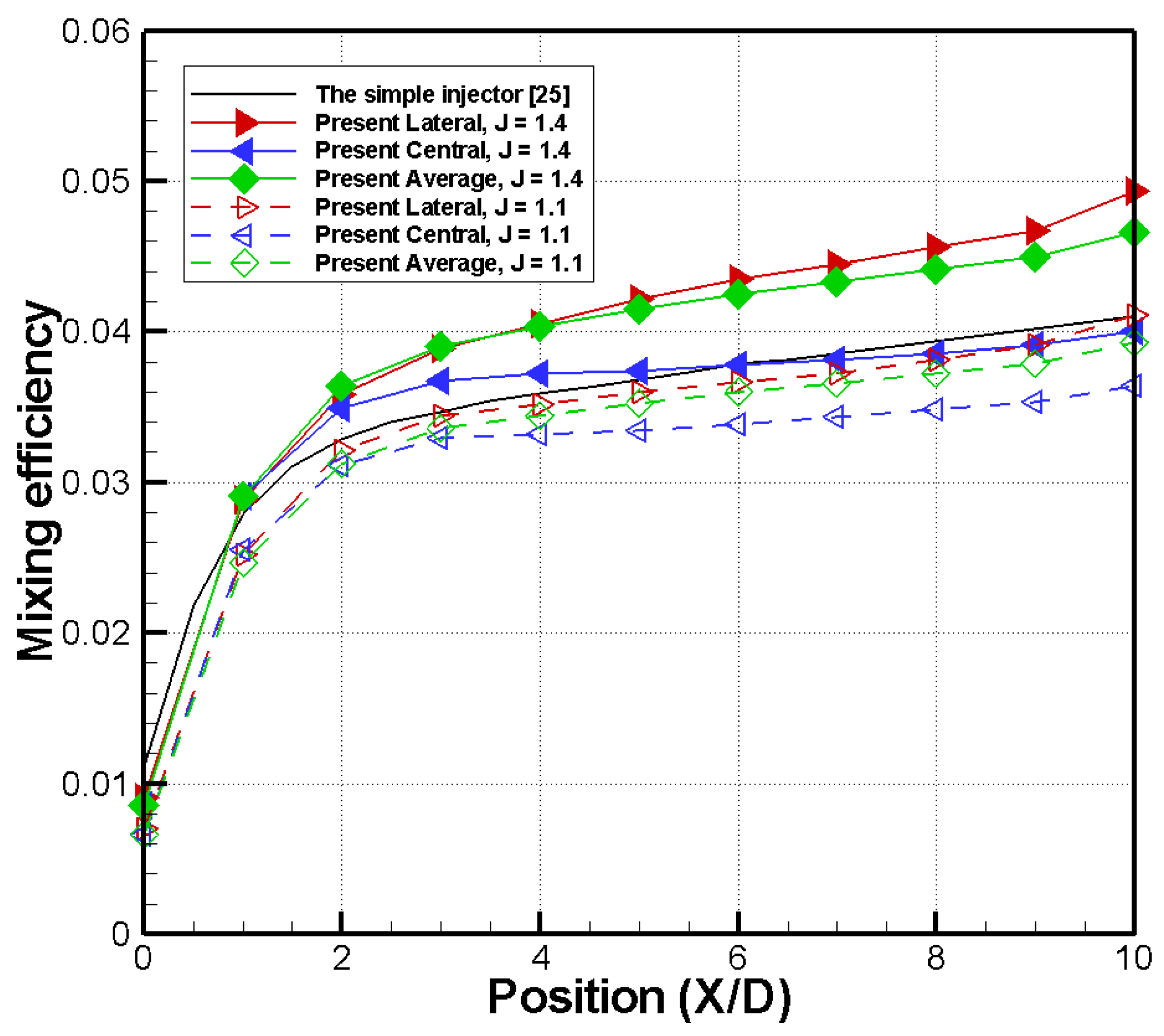
Figure 16 presents mixing efficiency along the x-axis. The red and blue lines are the results obtained with lateral injection and central injection, respectively. The green line is the average value for one cycle. There is no significant difference between the value obtained with lateral injection and the time-averaged value, but the value obtained with central injection shows significantly lower efficiency than the other two values. This occurs because the duration of lateral injection, which has high mixing efficiency, is longer than that of central injection.
The time-averaged value of the mixing efficiency in cases with J = 1.4 improved by about 17% compared to the result with the simple injector, meaning that higher efficiency can be expected under the same momentum flux ratio conditions at the outlet. However, the mixing efficiency of the cases with J = 1.1 decreases. This is due to the loss of total pressure in the fluidic oscillator, which reduced the mass flow rate and momentum at the outlet. In conclusion, higher mixing performance can be expected when using the fluidic oscillator with the same amount of fuel consumption. However, this requires a higher-pressure supply compared to simple injectors, and the application of the same total pressure at the inlet may reduce the mixing performance.
4. Conclusions
Numerical simulations were conducted to investigate the possibility of using a fluidic oscillator as a fuel injection device in a supersonic flow field. The simulation results were compared with the previous results to validate that the numerical methods, and fuel-injected in a supersonic flow field were simulated to observe the flow structure, fuel distribution, and various mixing characteristics. The fluidic oscillator was confirmed to improve the air–fuel mixing characteristics. However, oscillations of the flow are related to the generation of the recirculation zone inside of the fluidic oscillator, which results in losses of total pressure and momentum. When fuel is injected using the fluidic oscillator, the fuel distribution continues to vary over time. The fuel distribution forms a narrow and long structure when the fuel is injected laterally, but the result is similar to that of a simple injector when the injection is transverse.
The bow shock was formed further downstream when using the fluidic oscillator, but it expanded widely in the lateral direction. The size and shape of the horseshoe vortex varied with the injected direction, and they were smaller than those obtained with a simple injection. The results showed that the fluidic oscillator enhanced the mixing performance compared to that of a simple injector when injecting the same mass flow rate of fuel. This means that the same amount of fuel is consumed. In this case, the time-averaged penetration length and the area of the flammable region were largely increased. Furthermore, the mixing efficiency increases. The results suggest that the fluidic oscillator can be applied as an injector for a supersonic combustor to enhance the mixing efficiency.
When a supersonic fluidic oscillator was applied as a fuel injector of a supersonic combustor, a higher air–fuel mixing performance could be expected, but a disadvantage of increasing total pressure loss was also observed. For more practical applications, it is necessary to verify the validity of the computational simulation results through experimental studies. Furthermore, it is also necessary to observe interaction phenomena when several fluidic oscillators are applied simultaneously.
Author Contributions
Conceptualization, E.C.L. and H.J.L.; data curation, E.C.L.; formal analysis, T.-S.R.; funding acquisition, T.-S.R.; investigation, E.C.L., S.-W.C., H.-S.K., and H.J.L.; methodology, E.C.L., T.-S.R., and H.J.L.; project administration, H.J.L.; resources, H.J.L.; software, E.C.L. and S.-W.C.; supervision, H.J.L.; validation, E.C.L., S.-W.C., and H.J.L.; visualization, E.C.L. and S.-W.C.; writing—original draft, E.C.L.; writing—review and editing, T.-S.R. and H.J.L.
Funding
This research received no external funding.
Acknowledgments
This work was supported by the National Research Foundation of Korea (NRF) grant funded by the Korea government(MSIT) (NRF-2013R1*_A5_*A1073861).
Conflicts of Interest
The authors declare no conflict of interest.
References
- Ferri, A. Possible directions of future research in air-breathing engines. In Proceedings of the Fourth Agard Colloquium on Combustion and Propulsionm, Milan, Italy, 4–8 April 1960; pp. 3–15. [Google Scholar]
- Seiner, J.M.; Dash, S.M.; Kenzakowski, D.C. Historical survey on enhanced mixing in scramjet engines. J. Propuls. Power 2001, 17, 1273–1286. [Google Scholar] [CrossRef]
- Gruber, M.R.; Carter, C.D.; Montes, D.R.; Haubelt, L.C.; King, P.I.; Hsu, K.Y. Experimental studies of pylon-aided fuel injection into a supersonic crossflow. J. Propuls. Power 2008, 24, 460–470. [Google Scholar] [CrossRef] [Green Version]
- Doster, J.; King, P.; Gruber, M.; Maple, R. Pylon fuel injector design for a scramjet combustor. In Proceedings of the 43rd AIAA/ASME/SAE/ASEE Joint Propulsion Conference & Exhibit, Cincinnati, OH, USA, 8–11 July 2007; p. 5404. [Google Scholar]
- Takahashi, H.; Tu, Q.; Segal, C. Effects of pylon-aided fuel injection on mixing in a supersonic flowfield. J. Propuls. Power 2010, 26, 1092–1101. [Google Scholar] [CrossRef]
- Gruenig, C.; Avrashkov, V.; Mayinger, F. Fuel injection into a supersonic airflow by means of pylons. J. Propuls. Power 2000, 16, 29–34. [Google Scholar] [CrossRef]
- Yu, K.H.; Wilson, K.J.; Schadow, K.C. Effect of flame-holding cavities on supersonic-combustion performance. J. Propuls. Power 2001, 17, 1287–1295. [Google Scholar] [CrossRef]
- Kim, K.M.; Baek, S.W.; Han, C.Y. Numerical study on supersonic combustion with cavity-based fuel injection. Int. J. Heat Mass Transf. 2004, 47, 271–286. [Google Scholar] [CrossRef]
- Huang, W.; Wang, Z.G.; Yan, L.; Liu, W.D. Numerical validation and parametric investigation on the cold flow field of a typical cavity-based scramjet combustor. Acta Astronaut. 2012, 80, 132–140. [Google Scholar] [CrossRef]
- Heller, H.H.; Bliss, D.B. Flow-induced pressure fluctuations in cavities and concepts for their suppression. Aeroacoustics 1976, 45, 281–296. [Google Scholar]
- Zhang, X.; Edwards, J.A. Experimental investigation of supersonic flow over two cavities in tandem. AIAA J. 1992, 30, 1182–1190. [Google Scholar] [CrossRef]
- Ben-yakar, A.; Hanson, R.K. Cavity flame-holders for ignition and flame stabilization in scramjets: An overview. J. Propuls. Power 2001, 17, 869–877. [Google Scholar] [CrossRef]
- Ben-yakar, A.; Hanson, R. Supersonic combustion of cross-flow jets and the influence of cavity flame-holders. In Proceedings of the 37th Aerospace Sciences Meeting and Exhibit, Reno, NV, USA, 11–14 January 1999; p. 484. [Google Scholar]
- Freeborn, A.; King, P.; Gruber, M. Characterization of pylon effects on a scramjet cavity flameholder flowfield. In Proceedings of the 46th AIAA Aerospace Sciences Meeting and Exhibit, Reno, NV, USA, 7–10 January 2008; p. 86. [Google Scholar]
- Kim, C.H.; Jeung, I.S.; Choi, B.; Kouchi, T.; Masuya, G. Effect of Fuel Injection Locations with a Hyper Mixer in Supersonic Combustion. In Proceedings of the 47th AIAA/ASME/SAE/ASEE Joint Propulsion Conference & Exhibit, San Diego, CA, USA, 31 July–3 August 2011; p. 5830. [Google Scholar]
- Yamauchi, Y.; Kodama, Y.; Sakaue, S.; Arai, T. Effect of Mach Number on Supersonic Mixing by” Hyper-Mixer Injector”. In Proceedings of the 18th AIAA/3AF International Space Planes and Hypersonic Systems and Technologies Conference, Tours, France, 24–28 September 2012; p. 5816. [Google Scholar]
- Arai, T.; Sakaue, S.; Hayase, H.; Hiejima, T.; Sunami, T.; Nishioka, M. Streamwise Vortices Introduced by’Hyper-Mixer’on Supersonic Mixing. In Proceedings of the 17th AIAA International Space Planes and Hypersonic Systems and Technologies Conference, San Francisco, CA, USA, 11–14 April 2011; p. 2342. [Google Scholar]
- Kubo, N.; Tomioka, S.; Murakami, A.; Kudo, K. Mixing and combustion experiments with hyper-mixer injectors in a scramjet combustor. In Proceedings of the 50th AIAA/ASME/SAE/ASEE Joint Propulsion Conference, Cleveland, OH, USA, 28–30 July 2014; p. 3873. [Google Scholar]
- Doster, J.; King, P.; Gruber, M.; Maple, R. Numerical simulation of ethylene injection from in-stream fueling pylons. In Proceedings of the 15th AIAA International Space Planes and Hypersonic Systems and Technologies Conference, Dayton, OH, USA, 28 April–2 May 2008; p. 2518. [Google Scholar]
- Desikan, S.L.N.; Kumaran, K.; Babu, V. Numerical investigation of the role of hyper-mixers in supersonic mixing. Aeronaut. J. 2010, 114, 659–672. [Google Scholar] [CrossRef] [Green Version]
- Desikan, S.L.; Kurian, J. Strut-based gaseous injection into a supersonic stream. J. Propuls. Power 2006, 22, 474–477. [Google Scholar] [CrossRef]
- Ebrahimi, H.; Malo-molina, F.J.; Gaitonde, D.V. Numerical simulation of injection strategies in a cavity-based supersonic combustor. J. Propuls. Power 2012, 28, 991–999. [Google Scholar] [CrossRef]
- Mcclinton, C.R. The Effect of Injection Angle on the Interaction between Sonic Secondary Jets and a Supersonic Free Stream; NASA Langley Research Center: Hampton, VA, USA, 1972.
- Ogawa, H. Effects of injection angle and pressure on mixing performance of fuel injection via various geometries for upstream-fuel-injected scramjets. Acta Astronaut. 2016, 128, 485–498. [Google Scholar] [CrossRef]
- Kim, S.; Lee, B.J.; Jeung, I.S.; Lee, H. Characteristics of the Transverse Fuel Injection into a Supersonic Crossflow using Various Injector Geometries. J. Korean Soc. Propuls. Eng. 2018, 22, 53–64. [Google Scholar] [CrossRef]
- Paschereit, C.O.; Gutmark, E.; Weisenstein, W. Excitation of thermoacoustic instabilities by interaction of acoustics and unstable swirling flow. AIAA J. 2000, 38, 1025–1034. [Google Scholar] [CrossRef]
- Strykowski, P.J.; Krothapalli, A.; Wishart, D. Enhancement of mixing in high-speed heated jets using a counterflowing nozzle. AIAA J. 1993, 31, 2033–2038. [Google Scholar] [CrossRef]
- Randolph, H.; Chew, L.; Johari, H. Pulsed jets in supersonic crossflow. J. Propuls. Power 1994, 10, 746–748. [Google Scholar] [CrossRef]
- Chen, S.; Zhao, D. RANS investigation of the effect of pulsed fuel injection on scramjet HyShot II engine. Aerosp. Sci. Technol. 2019, 84, 182–192. [Google Scholar] [CrossRef]
- Cutler, A.D.; Harding, G.C.; Diskin, G.S. High frequency pulsed injection into a supersonic duct flow. AIAA J. 2013, 51, 809–818. [Google Scholar] [CrossRef]
- Milton, B.E.; Pianthong, K. Pulsed, supersonic fuel jets—A review of their characteristics and potential for fuel injection. Int. J. Heat Fluid Flow 2005, 26, 656–671. [Google Scholar] [CrossRef]
- Kouchi, T.; Sasaya, K.; Watanabe, J.; Shibayama, H.; Masuya, G. Penetration characteristics of pulsed injection into supersonic crossflow. In Proceedings of the 46th AIAA/ASME/SAE/ASEE Joint Propulsion Conference & Exhibit, Nashville, TN, USA, 25–28 July 2010; p. 6645. [Google Scholar]
- Kouchi, T.; Sakuranaka, N.; Izumikawa, M.; Tomioka, S. Pulsed transverse injection applied to a supersonic flow. In Proceedings of the 43rd AIAA/ASME/SAE/ASEE Joint Propulsion Conference & Exhibit, Cincinnati, OH, USA, 8–11 July 2007; p. 5405. [Google Scholar]
- Murugappan, S.; Gutmark, E. Parametric study of the Hartmann—Sprenger tube. Exp. Fluids 2005, 38, 813–823. [Google Scholar] [CrossRef]
- Gu, H.; Zhi, L.; Chen, L.; Gu, S.; Chang, X. Characteristics of Supersonic Combustion with Hartmann-Sprenger Tube Aided Fuel Injection. In Proceedings of the 17th AIAA International Space Planes and Hypersonic Systems and Technologies Conference, San Francisco, CA, USA, 11–14 April 2011; p. 2326. [Google Scholar]
- Elshamy, O.; Tambe, S.; Cai, J.; Jeng, S.M. Excited liquid jets in subsonic crossflow. In Proceedings of the 45th AIAA Aerospace Sciences Meeting and Exhibit, Reston, VA, USA, 8–11 January 2007; p. 1340. [Google Scholar]
- Song, Y.; Hwang, D.; Ahn, K. Spray characteristics of liquid jets in acoustically-forced crossflows. J. Korean Soc. Propuls. Eng. 2018, 22, 1–10. [Google Scholar] [CrossRef]
- Viets, H. Flip-flop jet nozzle. AIAA J. 1975, 13, 1375–1379. [Google Scholar] [CrossRef]
- Wiltse, J.M.; Glezer, A. Direct excitation of small-scale motions in free shear flows. Phys. Fluids 1998, 10, 2026–2036. [Google Scholar] [CrossRef]
- Lee, S.; Park, S.; Kang, M.; Lee, Y. Influences of the Internal Geometry of the Fluidic Oscillator on the Characteristics of Supersonic Sweeping Jet. Trans. Korean Soc. Mech. Eng. B 2019, 43, 99–107. [Google Scholar] [CrossRef]
- Gregory, J.; Tomac, M.N. A review of fluidic oscillator development. In Proceedings of the 43rd AIAA Fluid Dynamics Conference, San Diego, CA, USA, 24–27 June 2013; p. 2474. [Google Scholar]
- Gokoglu, S.; Kuczmarski, M.; Culley, D.; Raghu, S. Numerical studies of a supersonic fluidic diverter actuator for flow control. In Proceedings of the 5th Flow Control Conference, Chicago, IL, USA, 28 June 2010; p. 4415. [Google Scholar]
- Raman, G.; Raghu, S. Cavity resonance suppression using miniature fluidic oscillators. AIAA J. 2004, 42, 2608–2612. [Google Scholar] [CrossRef]
- Ben-yakar, A.; Mungal, M.G.; Hanson, R.K. Time evolution and mixing characteristics of hydrogen and ethylene transverse jets in supersonic crossflows. Phys. Fluids 2006, 18, 026101. [Google Scholar] [CrossRef] [Green Version]
- Rdem, E.; Kontis, K. Numerical and experimental investigation of transverse injection flows. Shock Waves 2010, 20, 103–118. [Google Scholar]
- Fiorina, B.; Lele, S. Numerical investigation of a transverse jet in a supersonic crossflow using large eddy simulation. In Proceedings of the 36th AIAA Fluid Dynamics Conference and Exhibit, San Francisco, CA, USA, 5–8 June 2006; p. 3712. [Google Scholar]
- You, Y.; Luedeke, H.; Hannemann, K. Injection and mixing in a scramjet combustor: DES and RANS studies. Proc. Combust. Inst. 2013, 34, 2083–2092. [Google Scholar] [CrossRef]
- Won, S.H.; Jeung, I.S.; Parent, B.; Choi, J.Y. Numerical investigation of transverse hydrogen jet into supersonic crossflow using detached-eddy simulation. AIAA J. 2010, 48, 1047–1058. [Google Scholar] [CrossRef]
- Won, S.H.; Jeung, I.S.; Choi, J.Y. Verification and Validation of the Numerical Simulation of Transverse Injection Jets using Grid Convergence Index. J. Korean Soc. Aeronaut. Space Sci. 2006, 34, 53–62. [Google Scholar]
- Mcdaniel, J.C.; Raves, J. Laser-induced-fluorescence visualization of transverse gaseous injection in a nonreacting supersonic combustor. J. Propuls. Power 1988, 4, 591–597. [Google Scholar] [CrossRef]
- Gruber, M.R.; Nejadt, A.S.; Chen, T.H.; Dutton, J.C. Mixing and penetration studies of sonic jets in a Mach 2 freestream. J. Propuls. Power 1995, 11, 315–323. [Google Scholar] [CrossRef]
- Faucher, J.; Joseph, E.; Goldstein, S.; Tabach, E. Supersonic Combustion of Fuels Other than Hydrogen for Scramjet Application; Technical Report AFAPL-TR-67-12; US Air Force: East Hartford, CT, USA, 1967. [Google Scholar]
- Mao, M.; Riggins, D.W.; Mcclinton, C.R. Numerical Simulation of Transverse Fuel Injection; NASA Langley Research Center: Hampton, VA, USA, 1991.
Figure 1.
Fluidic oscillator with feedback channel.
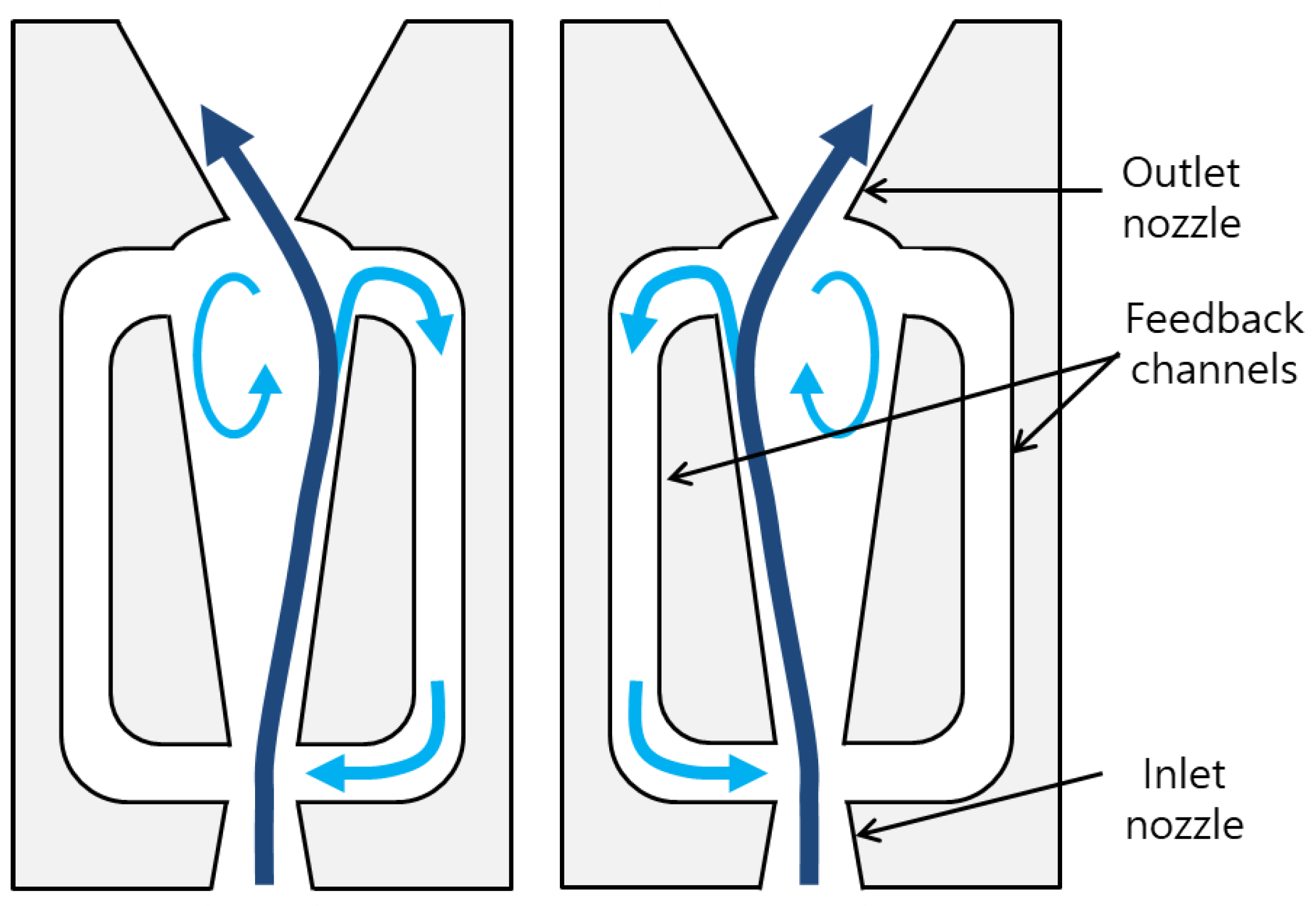
Figure 2.
Computational domain and boundary conditions: (a) entire domain; (b) fluidic oscillator.
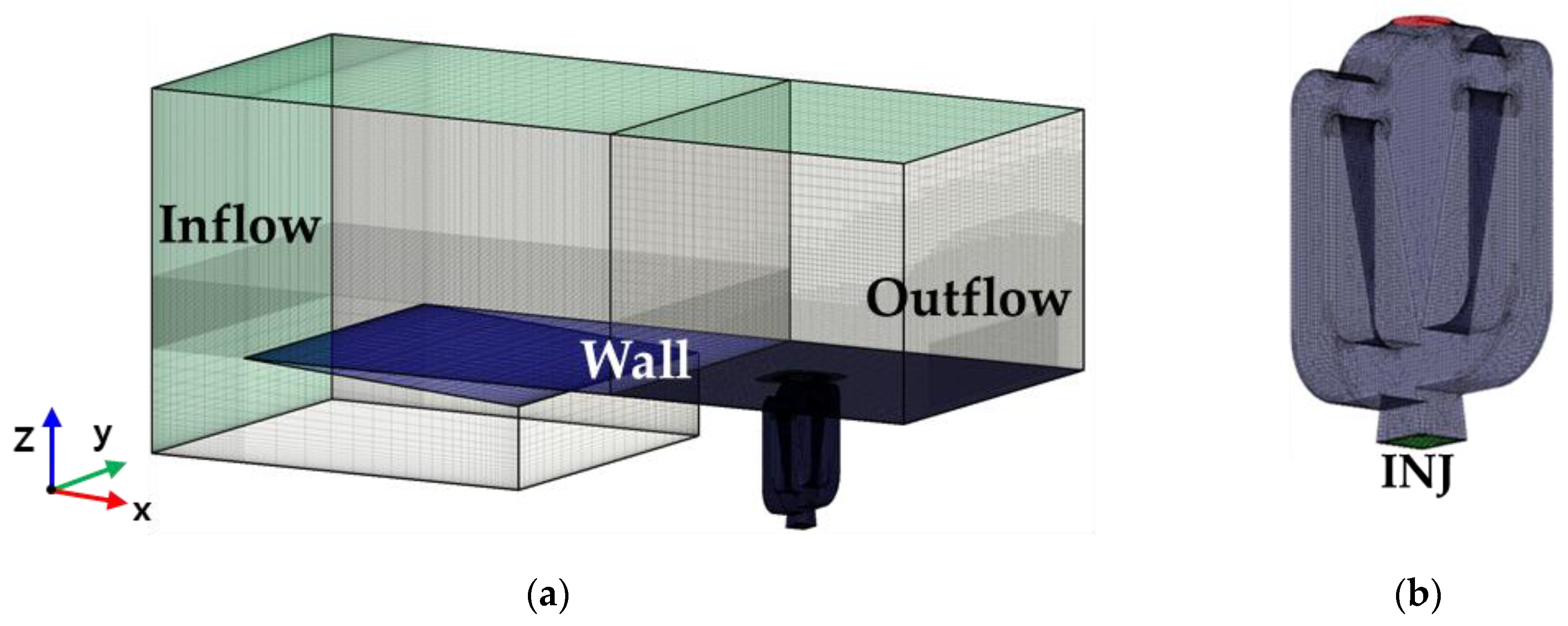
Figure 3.
Comparisons of flow structure in the fluidic oscillator: (a) experimental Schlieren image; (b) density gradient; (c) Mach number; (d) pressure.
Figure 3.
Comparisons of flow structure in the fluidic oscillator: (a) experimental Schlieren image; (b) density gradient; (c) Mach number; (d) pressure.
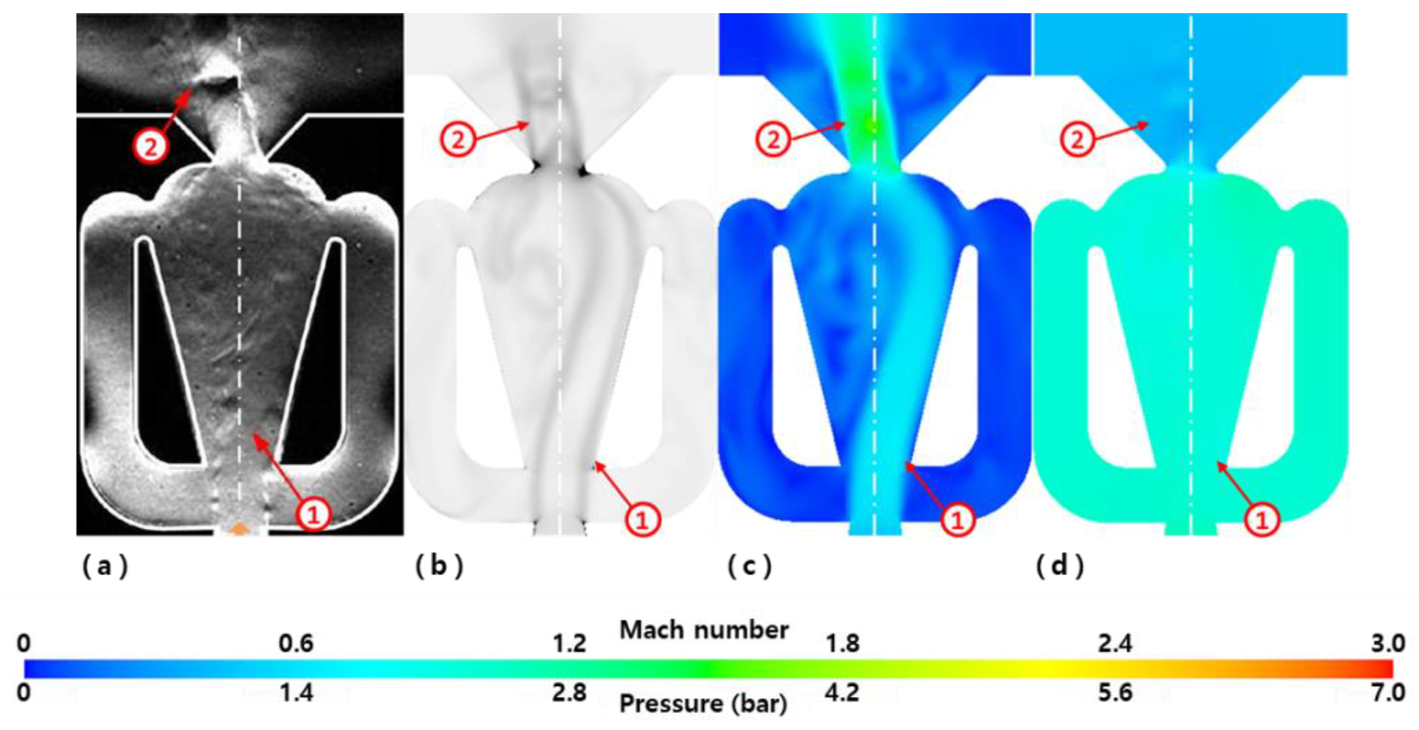
Figure 4.
Properties of injector outlet flow: (a) mass flow rate; (b) total pressure for one cycle.

Figure 5.
Total pressure recovery inside the fluidic oscillator of two cases (J = 1.1, 1.4) for one cycle.
Figure 5.
Total pressure recovery inside the fluidic oscillator of two cases (J = 1.1, 1.4) for one cycle.

Figure 6.
Fuel () distribution and flow structure along the x-axis.
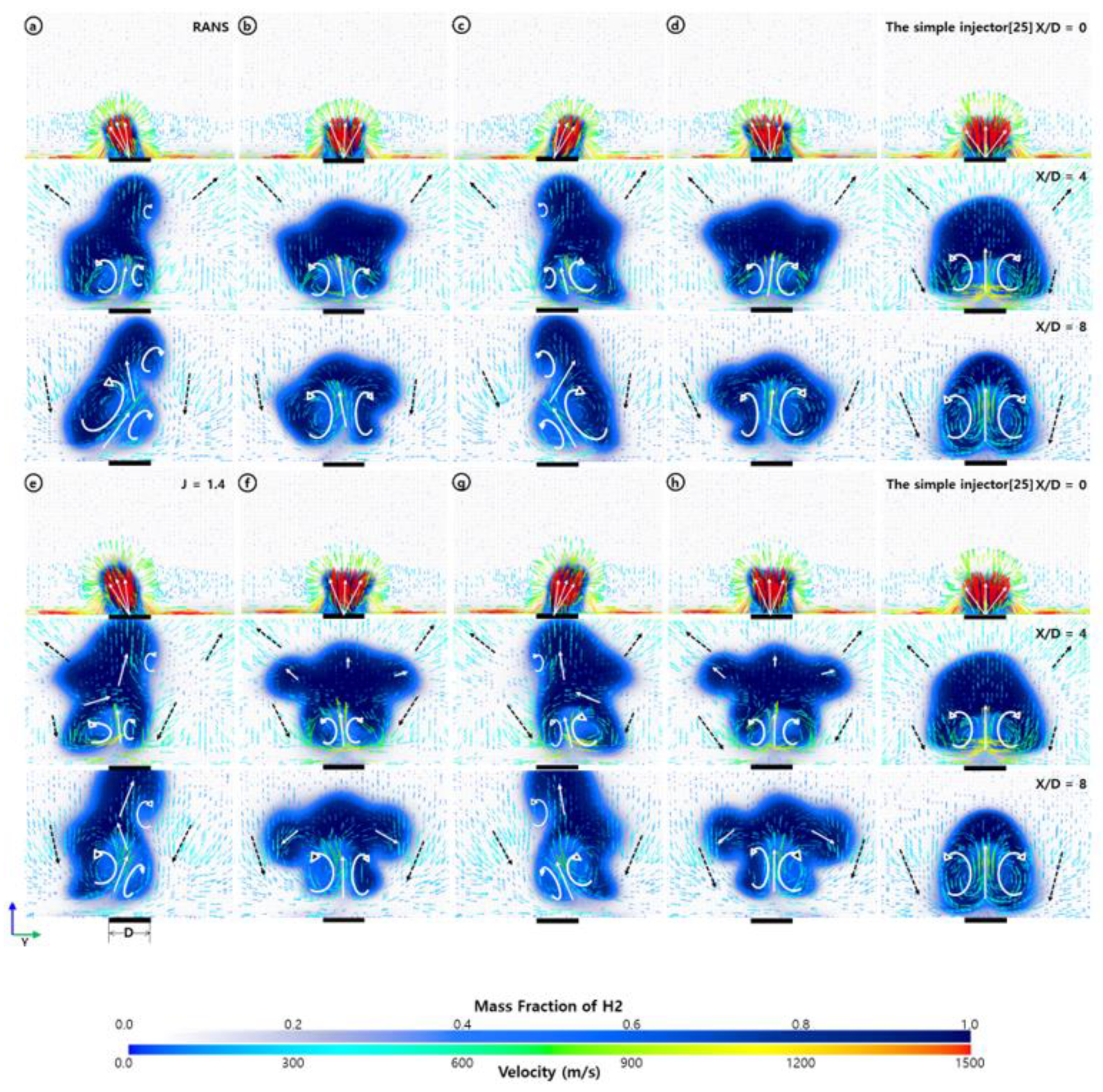
Figure 7.
Streamlines of fuel jet on yz-plane.

Figure 8.
Streamlines of fuel jet on xy-plane.
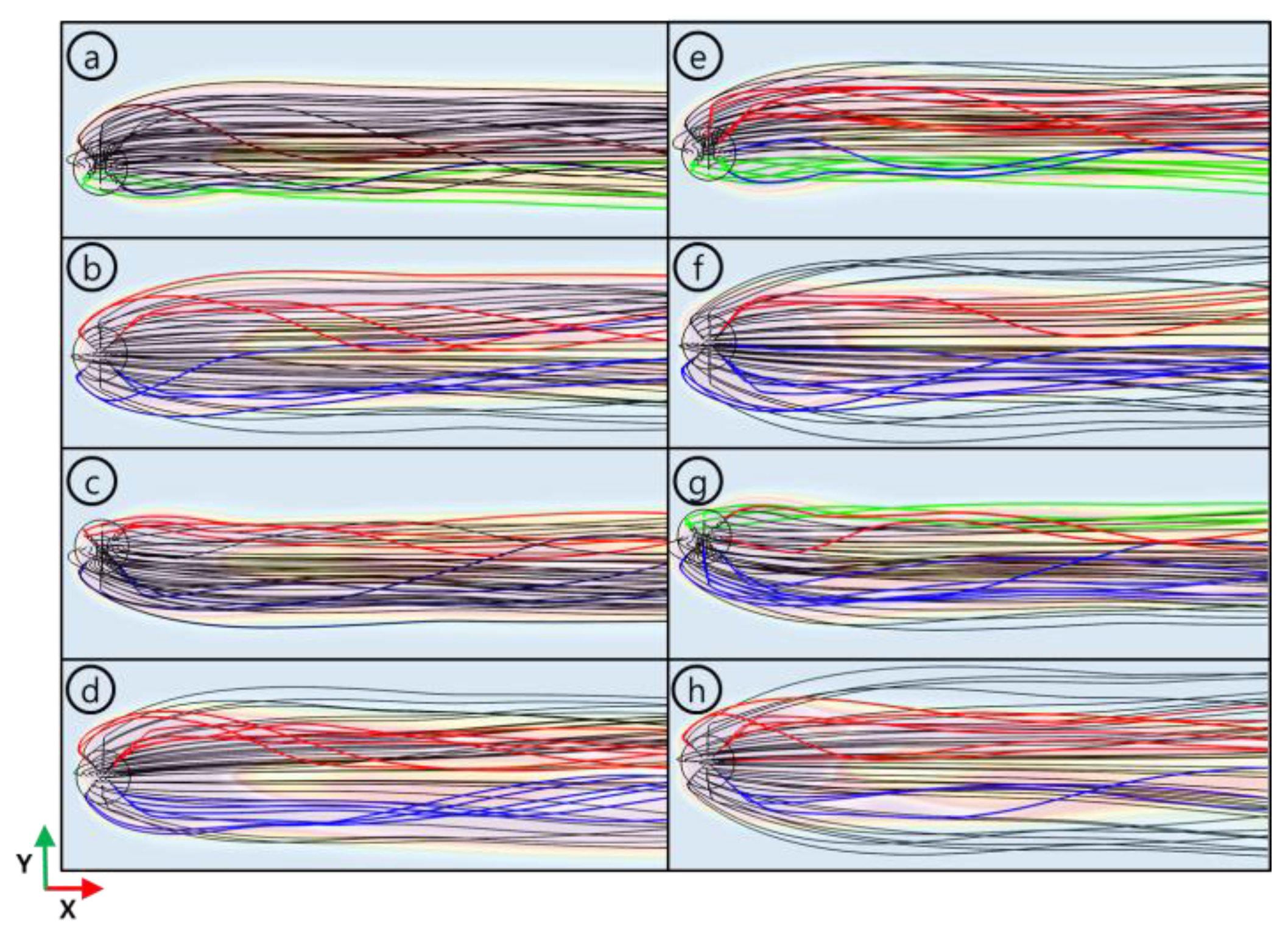
Figure 9.
Total pressure recovery of the flow fields along the z-axis (J = 1.1).

Figure 10.
Total pressure recovery of the flow fields along the z-axis (J = 1.4).
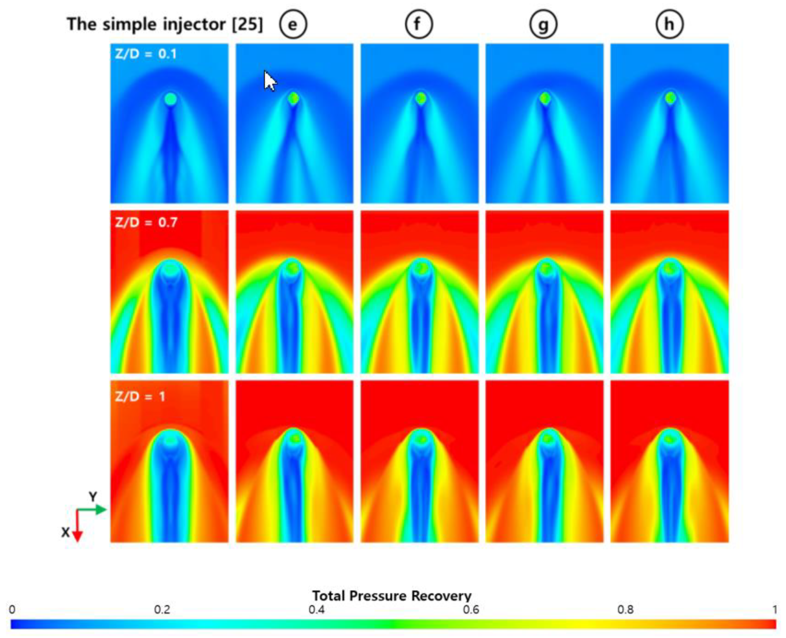
Figure 11.
Comparison of fuel penetration length along the x-axis.

Figure 12.
Comparison of area of the flammable region along the x-axis.

Figure 13.
Comparison of the flammable region at J = 1.1.

Figure 14.
Comparison of the flammable region at J = 1.4.
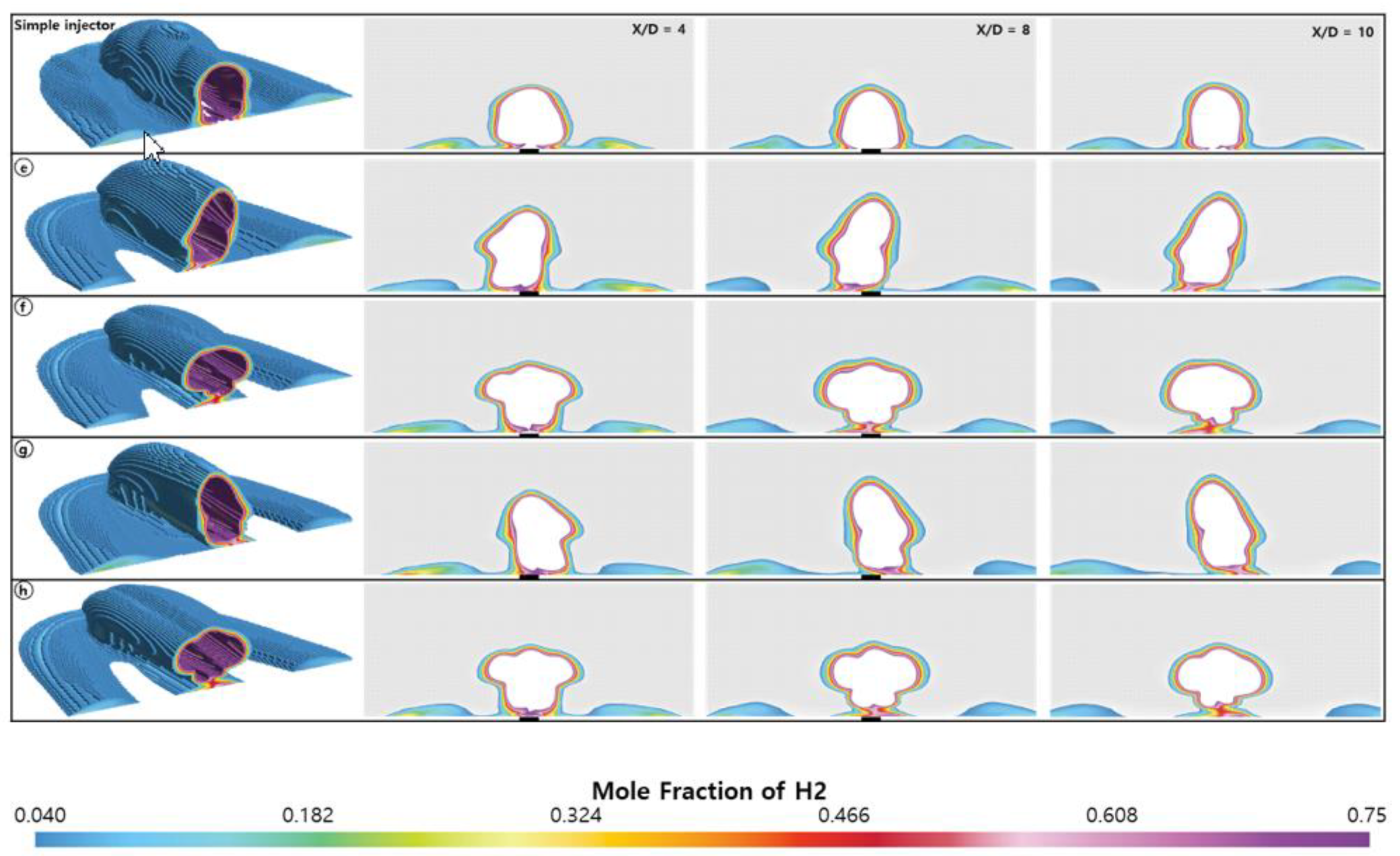
Figure 15.
Comparison of total pressure loss along the x-axis.

Figure 16.
Comparison of mixing efficiency along the x-axis.

Table 1.
Flow conditions of Inflow and injected fuel ().
| Inflow Conditions (Freestream) | Injection Conditions (INJ) | |||
|---|---|---|---|---|
| Reference [25] | Present Study Using the Fluidic Oscillator | |||
| Mach number | 3.38 | J = 1.4 | J = 1.1 | J = 1.4 |
| Total temperature (K) | 4237 | 295 | ||
| Total pressure (bar) | 20.81 | 9.28 | 9.275 @ inlet | 11.92 @ inlet |
| Mass flow rate (g/s) | 1.82 | 1.42 (time averaged) | 1.82 (time averaged) | |
| Reynolds number | 2.2 × 10⁵ | 1.5 × 10⁵ | 7.0 × 10⁴ @ outlet | 9.0 × 10⁴ @ outlet |
Table 2.
Oscillating characteristics of the flow using the fluidic oscillator.
| Frequency (Hz) | Sweeping Angle (°) | |
|---|---|---|
| Lee et al. [40] | 600 | 20 |
| Present result | 599.94 | 20 |
© 2019 by the authors. Licensee MDPI, Basel, Switzerland. This article is an open access article distributed under the terms and conditions of the Creative Commons Attribution (CC BY) license (http://creativecommons.org/licenses/by/4.0/).
Share and Cite
MDPI and ACS Style
Lee, E.C.; Cha, S.-W.; Kwon, H.-S.; Roh, T.-S.; Lee, H.J. A Numerical Study on the Characteristics of Air–Fuel Mixing Using a Fluidic Oscillator in Supersonic Flow Fields. Energies 2019, 12, 4758. https://doi.org/10.3390/en12244758
AMA Style
Lee EC, Cha S-W, Kwon H-S, Roh T-S, Lee HJ. A Numerical Study on the Characteristics of Air–Fuel Mixing Using a Fluidic Oscillator in Supersonic Flow Fields. Energies. 2019; 12(24):4758. https://doi.org/10.3390/en12244758
Chicago/Turabian StyleLee, Eun Cheol, Seung-Won Cha, Hee-Soo Kwon, Tae-Seong Roh, and Hyoung Jin Lee. 2019. "A Numerical Study on the Characteristics of Air–Fuel Mixing Using a Fluidic Oscillator in Supersonic Flow Fields" Energies 12, no. 24: 4758. https://doi.org/10.3390/en12244758
Note that from the first issue of 2016, this journal uses article numbers instead of page numbers. See further details here.