Non-Iterative Methods for the Extraction of the Single-Diode Model Parameters of Photovoltaic Modules: A Review and Comparative Assessment

Abstract

The extraction of the photovoltaic (PV) model parameters remains to this day a long-standing and popular research topic. Numerous methods are available in the literature, widely differing in accuracy, complexity, applicability, and their very nature. This paper focuses on the class of non-iterative parameter extraction methods and is limited to the single-diode PV model. These approaches consist of a few straightforward calculation steps that do not involve iterations; they are generally simple and easy to implement but exhibit moderate accuracy. Seventeen such methods are reviewed, implemented, and evaluated on a dataset of more than one million measured I-V curves of six different PV technologies provided by the National Renewable Energy Laboratories (NREL). A comprehensive comparative assessment takes place to evaluate these alternatives in terms of accuracy, robustness, calculation cost, and applicability to different PV technologies. For the first time, the irregularities found in the extracted parameters (negative or complex values) and the execution failures of these methods are recorded and are used as an assessment criterion. This comprehensive and up-to-date literature review will serve as a useful tool for researchers and engineers in selecting the appropriate parameter extraction method for their application.

1. Introduction

The model of a photovoltaic (PV) generator usually consists of an equivalent circuit and a set of parameters that describe its electrical response and operation. Determination of these parameters is not a trivial task, as they are not available in the PV module’s datasheet and their values change with the operating conditions. Immense research has been carried out in recent decades on the extraction of the PV model parameters, the literature presenting numerous methods of different nature, reliability, complexity, and required input data. It now constitutes a research topic on its own, referred to as “PV cell model parameters estimation problem” or similar in the literature [1].

These methods can be classified into three major categories: the numerical, the non-iterative and the optimization approaches. The numerical (or iterative) methods form a system of a few equations which is solved numerically [2,3,4,5,6], in a trial-and-error manner or via another iterative algorithm [7,8,9,10]. These equations are usually derived by applying the PV model equation to specific conditions, such as short-circuit (SC), open-circuit (OC) or maximum power point (MPP). This class achieves generally high accuracy but suffers from initialization and convergence issues, high calculation cost and solution suboptimality [1,11,12,13]. The non-iterative (or explicit or direct or analytical) methods employ a set of equations as well, but are solved symbolically/explicitly (no iterations) resulting in simpler formulation and implementation [12,14,15,16,17,18,19,20,21,22,23,24,25,26,27,28]. These approaches are essentially variations of the numerical class that employ a series of simplifications and empirical observations to achieve explicit formulation. Quite often, they are used in the initialization step of the numerical methods [26,29]. It is worth noting that the term “analytical” is somehow ambiguous in the literature, referring either to the non-iterative, numerical, or both classes, thus it is not used in this paper to avoid confusion. The non-iterative methods are easier to implement and more computationally efficient but yield lower accuracy [13], although some of these approaches perform quite decently [30]. The optimization (or artificial intelligence or heuristic or curve-fitting or soft-computing) methods follow a non-technologically specific approach where the model’s equation is optimally fitted on a set of measurements, usually the I-V curve. Various evolution inspired [31,32,33] and curve-fitting [34,35] algorithms may be found in the literature. This class exhibits generally high accuracy and near-global optimality but suffers from computational complexity and difficulties in the method’s parameters tuning [1].

Another important aspect of a parameter extraction technique is the required input data. For some methods, the datasheet information suffices (e.g., SC, OC, and MPP data, temperature coefficients etc.) [12,15,17,20,21,22,25,26,27], while others require additional operating points or/and the slope of the I-V curve at SC or OC [14,16,18,19,23,24]. Generally, the former cases are preferable as they can be applied more easily and universally, not necessitating extra measurements [19,27,36]. Furthermore, there is currently a debate in the literature on whether the extracted parameters should be restricted to real positive numbers to have a physical meaning [4,26], or should be allowed to take negative or complex values (referred to as parameter irregularities in this paper) if the resulted curve better matches the measurements [15,30]. Other desirable attributes of such a method is to be accurate, robust, computationally efficient, and applicable to various PV technologies [1,27].

The large diversity in the requirements, performance and very nature of these methods has inspired the publication of several review papers in the literature [1,30,36,37,38,39,40,41]. The studies in [1,37] provide a qualitative description and classification of all three classes, but without implementation and quantitative comparison. The rest of the aforementioned papers are limited to the numerical or/and non-iterative methods, implementing and evaluating some of them. However, only a small subset of the available non-iterative methods is assessed, and the evaluation dataset corresponds mainly to single- and multi-crystalline silicon PV modules [30,36,38]. The copper indium gallium selenide (CIGS) and cadmium telluride (CdTe) technologies are considered in [39], heterojunction with intrinsic thin layer (HIT) modules are tested in [40] and a few multi-junction devices are examined in [41]. To this day, there is no comparative study in the literature to consider all the commercially available PV technologies. Furthermore, although the robustness has been investigated in the numerical and optimization classes, the aspect of execution failure or irregular results in the non-iterative methods has not been studied yet.

To shed some light on these topics, this paper performs a comprehensive review and comparison of the non-iterative parameter extraction methods that are based on the single-diode PV model. Seventeen such methods are identified dating since 1984 [12,14,15,16,17,18,19,20,21,22,23,24,25,26,27], all of which are implemented and assessed on a common set of I-V curves provided by National Renewable Energy Laboratories (NREL) [42]. This dataset contains 1,025,665 I-V curves measured over a one-year period in the USA for 22 PV modules under a wide range of irradiance and temperature conditions. This is probably one of the most comprehensive publicly available datasets, including six different PV technologies: single- (c-Si) and multi-crystalline (mc-Si), CdTe, CIGS, HIT and amorphous silicon (a-Si) (crystalline, tandem, and triple-junction). It is worth noting that this investigation is limited to the single-diode PV model, adopted by most of the non-iterative parameter extraction methods, even though other more sophisticated models may be more appropriate for some thin-film technologies.

The comparison that follows aims to give the full picture on the appropriateness of the non-iterative methods in terms of accuracy, robustness, and calculation cost for all these PV technologies. Special focus is given on the execution failures recorded for the 1 million scenarios to evaluate their credibility, and the number of parameter irregularities (negative or complex values) that may be or may be not a limiting factor to some applications. The assessment is performed first for all 17 methods, and then separately for those that rely solely on datasheet information; furthermore, a sensitivity analysis takes place on the fitting range for the extraction of the SC slope. This survey is a thorough and up-to-date comparative assessment of the available non-iterative methods, carried out for the first time on a comprehensive dataset and accounting for the aspects of reliability and robustness.

The rest of the paper is organized as follows: the basics of the single-diode PV model are given in Section 2 and the non-iterative parameter extraction methods are described and discussed in Section 3. The performance of these methods is assessed and compared in Section 4, the main conclusions summarized in Section 5. The Appendix A and Appendix B clarifies some calculation aspects.

2. The Fundamentals of the Single-Diode PV Model

This section gives a brief description of the PV model theory under consideration; the following nomenclature is used throughout the paper for consistency. The single-diode model is historically the first PV model, developed initially for single-crystalline silicon PV cells, but it remains to this day the most commonly used one due to its simplicity [2,43,44]. Other more sophisticated models involve two [45] or three diodes [46] for increased accuracy at low irradiance, and sometimes additional voltage-dependent current sources to account for the breakdown operation [47] or the recombination phenomenon in some thin-film technologies [48]. This paper is limited to the single-diode model, as this is the PV model on which the majority of the non-iterative parameter extraction methods are based, and assesses its effectiveness on all commercial PV technologies, single/multi-crystalline silicon and thin-film.

This model consists of an equivalent circuit shown in Figure 1 and a set of five parameters $[I_{ph},I_s,a,R_s,R_{sh}]$:

• the photocurrent $I_{ph}$ (or $I_o$ or $I_{pv}$)
• the diode saturation current $I_s$ (or $I_o$ or $I_{sat}$)
• the modified diode factor a (or m)
• the series resistance $R_s$
• the shunt resistance $R_{sh}$ (or $R_p$).

Quite often, the modified diode factor a is expressed alternatively as $N_{s}n{V}_T$ in the literature, where $N_s$ is the number of series-connected cells, n the diode factor and $V_T=\frac{kT}{q}$ the thermal voltage (k is the Boltzmann constant, T the temperature in Kelvin and q the electron charge). The five parameters depend on both the structural characteristics of the PV modules and the operating conditions: incident irradiance and cell temperature. The irradiance is usually considered to affect proportionally $I_{ph}$ [1,2,3,4,7,20,21,27,28,36,43,49,50,51,52,53,54], and $R_{sh}$ in an inversely proportional way [1,2,3,4,20,27,36,43,49,51,52,54]; the temperature effect is generally assumed to be weak and linear in $I_{ph}$, strong and exponential in $I_s$, and strong and proportional in a [1,2,3,4,7,20,21,27,36,43,49,50,51,52,53,54]. The dependence of $R_s$ is somewhat unclear, some studies assuming to remain constant [2,3,4,36,43,50,51,53,54] and others to depend on both irradiance and temperature [1,20,27,49,52]. Typically, the five parameters are not assumed to be affected by the operating point, i.e., they do not change along the I-V curve. For some technologies, however, it has been reported to vary with the current, especially the diode factor and series resistance; here, the former approach is considered which is adopted by all parameter extraction methods examined. Please note that sometimes the literature neglects one or both resistances for simplicity [11,15,17,21,22,55].

The current-voltage equation is given implicitly by

$$\begin{array}{c}\hfill I=I_{ph}-I_s\left(e^{\frac{V+I{R}_s}{a}}-1\right)-\frac{V+I{R}_s}{R_{sh}}.\end{array}$$

(1)

This equation cannot be solved symbolically and necessitates numerical solution, which raises some challenges during the evaluation. As an alternative, an equivalent explicit formulation has appeared lately in the literature, employing the principal branch of the Lambert W function $W_0\{.\}$ [25,56,57,58]

$$\begin{array}{c}\hfill I=\frac{R_{sh}(I_{ph}+I_s)-V}{R_s+R_{sh}}-\frac{a}{R_s}{W}_0\left\{\frac{R_s{R}_{sh}{I}_s}{a(R_s+R_{sh})}{e}^{\frac{R_s{R}_{sh}(I_{ph}+I_s)+R_{sh}V}{a(R_s+R_{sh})}}\right\}\end{array}$$

(2)

$$\begin{array}{c}\hfill V=R_{sh}(I_{ph}+I_s)-(R_s+R_{sh})I-a{W}_0\left\{\frac{R_{sh}{I}_s}{a}{e}^{\frac{R_{sh}(I_{ph}+I_s-I)}{a}}\right\}.\end{array}$$

(3)

One can directly find the current for a given value of voltage using (2) or the opposite via (3), which makes the calculation easy and straightforward, in contrast to (1). The Lambert W function is readily available in all computational platforms; more information on the computation of this function are given in Appendix A.

The single-diode model describes any PV generator under uniform operating conditions, from cell to array, after scaling properly the five parameters [43]; it does not apply to non-uniform operation, such as partial shading, mismatched conditions etc., when appropriate extensions to account for the bypass diodes are necessary. Usually, the five parameters are extracted for the PV module, using the module datasheet information as input data. In the general case, however, one can extract the five parameters for any PV generator, from cell to array, when the respective I-V curve measurements are available. To relate the array parameters $[I_{ph,arr},I_{s,arr},a_{arr},R_{s,arr},R_{sh,arr}]$ to the cell parameters $[I_{ph,cell},I_{s,cell},a_{cell},R_{s,cell},R_{sh,cell}]$ the following expressions can be used [4,21,34,41,54]:

$$\begin{array}{cc}\hfill I_{ph,arr}& =N_p{I}_{ph,cell}\hfill \end{array}$$

(4)

$$\begin{array}{cc}\hfill I_{s,arr}& =N_p{I}_{s,cell}\hfill \end{array}$$

(5)

$$\begin{array}{cc}\hfill a_{arr}& =N_s{a}_{cell}\hfill \end{array}$$

(6)

$$\begin{array}{cc}\hfill R_{s,arr}& =\frac{N_s}{N_p}{R}_{s,cell}\hfill \end{array}$$

(7)

$$\begin{array}{cc}\hfill R_{sh,arr}& =\frac{N_s}{N_p}{R}_{sh,cell},\hfill \end{array}$$

(8)

where $N_p$ and $N_s$ are the parallel- and series-connected PV cells within the array. These relations hold true for the other PV structures as well, such the string or module, properly changing the meaning of the respective terms; e.g., the module-cell relation is given by (4)–(8) if the terms for the array parameters are substituted by the module ones and $N_p,N_s$ meaning is modified to account for the cells within the module, rather than the array. A typical first-quadrant I-V curve (non-negative voltage and current) of a PV module at STC (standard test conditions) is shown in Figure 2, indicating the SC, the OC, and the MPP, as well as the tangent lines at SC and OC. Most of the non-iterative parameter extraction methods require as input data the coordinates of these points $(0,I_{sc}),(V_{oc},0)$ and $(V_{mp},I_{mp})$, as well as the so-called experimental resistances $R_{sho}$ and $R_{so}$ that relate to the slope of the tangent lines according to

$$\begin{array}{c}\hfill R_{sho}={\left.-\frac{dV}{dI}\right|}_{SC},R_{so}={\left.-\frac{dV}{dI}\right|}_{OC}.\end{array}$$

(9)

The extraction of these slopes from I-V curve measurements is discussed in Appendix B. Other data possibly needed by a parameter extraction method is the temperature coefficients of the SC current ${\alpha }_{Isc}$ and OC voltage ${\beta }_{Voc}$. Please note that these coefficients are used in normalized form ($K^{-1}$) in this paper (normalized on the nominal SC current and OC voltage, e.g., ${\beta }_{Voc}=-0.0034$ K${}^{-1}$, ${\alpha }_{Isc}=+0.0006$ K${}^{-1}$), rather than in absolute form ($A/K,V/K$), as the normalized coefficients do not considerably differ among PV modules of the same technology which facilitates comparison [59].

3. The Non-Iterative Parameter Extraction Methods

A rigorous review reveals that there are seventeen different non-iterative methods available for the parameter extraction of the single-diode PV model, given in chronological order and denoted by the name of their respective main author in

Table 1. Main attributes of the 17 non-iterative parameter extraction methods.

No	Ref.	Method	Year	Number of Parameters	Eval Steps	Datasheet Sufficient?	Input Data
1	[14]	Phang	1984	5	7		$I_{sc},V_{oc},I_{mp},V_{mp},R_{sho},R_{so}$
2	[15]	Sera	2008	4	4	🗸	$I_{sc},V_{oc},I_{mp},V_{mp}$
3	[16]	Saleem	2009	5	7		$I_{sc},V_{oc},V_{mp},I_{60},V_{60}$
4	[17]	Saloux	2011	3	3	🗸	$I_{sc},V_{oc},I_{mp},V_{mp}$
5	[12]	Accarino	2013	5	6	🗸	$I_{sc},V_{oc},I_{mp},V_{mp},{\alpha }_{Isc},{\beta }_{Voc},V_{oc0}$
6	[18]	Khan	2013	5	7		$I_{sc},V_{oc},I_{mp},V_{mp},R_{sho},R_{so}$
7	[19]	Cubas1	2014	5	8		$I_{sc},V_{oc},I_{mp},V_{mp},R_{sho}$
8	[19]	Cubas2	2014	5	8	🗸	$I_{sc},V_{oc},I_{mp},V_{mp}$
9	[56]	Cubas3	2014	5	9	🗸	$I_{sc},V_{oc},I_{mp},V_{mp}$
10	[20]	Bai	2014	5	11	🗸	$I_{sc},V_{oc},I_{mp},V_{mp}$
11	[21]	Aldwane	2014	4	4	🗸	$I_{sc},V_{oc},I_{mp},V_{mp}$
12	[22]	Cannizzaro	2014	4	8 or 11	🗸	$I_{sc},V_{oc},I_{mp},V_{mp}$
13	[23]	Toledo	2014	5	13		$I_{sc},V_{oc},I_{mp},V_{mp},I_{xx},R_{sho}$
14	[24]	Louzazni	2015	5	7		$I_{sc},V_{oc},I_{mp},V_{mp},R_{sho},R_{so}$
15	[25]	Batzelis	2016	5	8	🗸	$I_{sc},V_{oc},I_{mp},V_{mp},{\alpha }_{Isc},{\beta }_{Voc},V_{oc0}$
16	[26]	Hejri	2016	5	5	🗸	$I_{sc},V_{oc},I_{mp},V_{mp}$
17	[27]	Senturk	2017	5	7	🗸	$I_{sc},V_{oc},I_{mp},V_{mp}$

. These are the most clearly described methods in the literature that are applicable to any operating conditions; the ones intended only for STC are not included in this comparative assessment. It is worth noting that some of these methods are designed for single/multi-crystalline silicon technologies, assuming the silicon energy gap and a diode factor close to 1, but in this study, they are applied to all six PV technologies to assess their universal performance maintaining consistency with the original studies. Table 1 also shows the number of evaluation steps, the required input data and whether the datasheet information suffices, or additional measurements are needed. In the rest of this section, the evaluation steps of these methods are briefly described using the common nomenclature of Section 2; it is shown that there is significant overlap among the alternatives, sharing several equations in the exact or very similar form.

3.1. Phang [1984]

Historically, the first attempts to extract the PV model parameters appeared in the 1960s: they employed semilogarithmic plots of the I-V characteristic to extract some of the parameters and required experienced users. These techniques were evolved later to complete and easy-to-use parameter extraction methods based on explicit equations, rather than plotted curves; the first such non-iterative method was published by Phang et al. in 1984 [14], still performing quite decently as discussed later. The same authors published later a comparative study [60] and a seven-parameters extraction method [61], but [14] remains the original publication adopted in several studies in the literature, such as in [50,62]. First, $R_{sho}$ and $R_{so}$ are extracted from the I-V curve slopes at SC and OC (see Appendix B), and then the five parameters are calculated by evaluating the following equations in this order:

$$\begin{array}{c}{R}_{sh}=R_{sho}\hfill \end{array}$$

(10)

$$\begin{array}{c}a=\frac{V_{mp}-V_{oc}+R_{so}{I}_{mp}}{ln\left[\frac{I_{sc}-I_{mp}-\raisebox{1ex}{$V_{mp}$}\!\left/ \!\raisebox{-1ex}{$R_{sh}$}\right.}{I_{sc}-\raisebox{1ex}{$V_{oc}$}\!\left/ \!\raisebox{-1ex}{$R_{sh}$}\right.}\right]+\frac{I_{mp}}{I_{sc}-\raisebox{1ex}{$V_{oc}$}\!\left/ \!\raisebox{-1ex}{$R_{sh}$}\right.}}\hfill \end{array}$$

(11)

$$\begin{array}{c}{I}_s=\left(I_{sc}-\frac{V_{oc}}{R_{sh}}\right)e^{-\frac{V_{oc}}{a}}\hfill \end{array}$$

(12)

$$\begin{array}{c}{R}_s=R_{so}-\frac{a}{I_s}{e}^{-\frac{V_{oc}}{a}}\hfill \end{array}$$

(13)

$$\begin{array}{c}{I}_{ph}=I_{sc}\left(1+\frac{R_s}{R_{sh}}\right)+I_s\left(e^{\frac{I_{sc}{R}_s}{a}}-1\right)\hfill \end{array}$$

(14)

3.2. Sera [2008]

The method of Sera et al. [15], also adopted by Khezzar et al. [55], is a four-parameter model that neglects $R_{sh}$:

$$\begin{array}{c}{I}_{ph}=I_{sc}\hfill \end{array}$$

(15)

$$\begin{array}{c}a=\frac{2V_{mp}-V_{oc}}{ln\left(\frac{I_{sc}-I_{mp}}{I_{sc}}\right)+\frac{I_{mp}}{I_{sc}-I_{mp}}}\hfill \end{array}$$

(16)

$$\begin{array}{c}{R}_s=\frac{aln\left(\frac{I_{sc}-I_{mp}}{I_{sc}}\right)+V_{oc}-V_{mp}}{I_{mp}}\hfill \end{array}$$

(17)

$$\begin{array}{c}{I}_s=I_{sc}{e}^{-\frac{V_{oc}}{a}}\hfill \end{array}$$

(18)

It is worth noting that a typo found in [15] has been corrected in (16), while (18) is somewhat similar to the Phang’s (12).

3.3. Saleem [2009]

The method of Saleem [16] is based on an alternative formulation of the PV equation as a power law function. It requires two additional points as input data: at voltage equal to 60% of $V_{oc}$$(0.6V_{oc},I_{60})$ and at current equal to 60% of $I_{sc}$$(V_{60},0.6I_{sc})$. First, the auxiliary parameters $\gamma$ and m are calculated:

$$\begin{array}{c}\hfill \gamma =\frac{\frac{I_{60}}{I_{sc}}-0.4}{0.6},m=\frac{log\left(\frac{0.4-(1-\gamma )\frac{V_{60}}{V_{oc}}}{\gamma }\right)}{log\frac{V_{60}}{V_{oc}}},\end{array}$$

(19)

and then the five parameters are found by

$$\begin{array}{c}a=\frac{V_{oc}}{m}\frac{0.77m(1-\frac{V_{mp}}{V_{oc}})-1}{0.77mln\frac{V_{oc}}{V_{mp}}-1}\hfill \end{array}$$

(20)

$$\begin{array}{c}{R}_s=\frac{V_{oc}}{0.6\gamma m{I}_{sc}}\left(1-\frac{am}{V_{oc}}\right)-0.1\hfill \end{array}$$

(21)

$$\begin{array}{c}{I}_s=\gamma I_{sc}{e}^{-\frac{V_{oc}}{a}}\hfill \end{array}$$

(22)

$$\begin{array}{c}{R}_{sh}=\frac{V_{oc}}{I_{sc}}\frac{1}{1-\gamma -\frac{\gamma }{0.6}exp\left[\frac{(0.4+0.6\gamma )I_{sc}{R}_s-0.4V_{oc}}{a}\right]}\hfill \end{array}$$

(23)

$$\begin{array}{c}{I}_{ph}=I_{sc}\left(1+\frac{R_s}{R_{sh}}\right).\hfill \end{array}$$

(24)

Note the logarithm with a base of 10 in (19) and the natural logarithm in (20).

3.4. Saloux [2011]

An explicit PV model based on the ideal single-diode equivalent (no resistances) is presented in [17]. Saloux provides some equations to determine the three parameters at STC, but it seems that they are applicable to other conditions as well, as slightly manipulated here:

$$\begin{array}{c}a=\frac{V_{mp}-V_{oc}}{ln\left(1-\frac{I_{mp}}{I_{sc}}\right)}\hfill \end{array}$$

(25)

$$\begin{array}{c}{I}_{ph}=I_{sc}\hfill \end{array}$$

(26)

$$\begin{array}{c}{I}_s=\frac{I_{sc}}{e^{\frac{V_{oc}}{a}}-1}.\hfill \end{array}$$

(27)

Apparently, the expressions for $I_{ph}$ and $I_s$ are almost the same as (15) and (18) from Sera’s model.

3.5. Accarino [2013]

This is the first extraction method to employ the Lambert W function [12]. First a is calculated via

$$\begin{array}{c}a=\frac{\left({\beta }_{Voc}-\frac{1}{T_0}\right)V_{oc0}}{{\alpha }_{Isc}-\frac{3}{T_0}-\frac{E_g}{k{T}_0^2}}\frac{T}{T_0},\hfill \end{array}$$

(28)

where $V_{oc0}$ is the nominal OC voltage (STC), $T_0=298.15$ K is the nominal temperature, $E_g=1.8e-19$ J the energy gap of silicon and $k=1.38e-23$ J/K${}^2$ the Boltzmann constant. Also note that the temperature coefficients are in normalized form. Then, $I_{ph}$ and $I_s$ are found by (15) and (18) from Sera’s model. Finally, the auxiliary parameter x is evaluated (after correcting a typo in [12]), used subsequently to calculate $R_s$ and $R_{sh}$:

$$\begin{array}{c}x=W_0\left\{\frac{V_{mp}(2I_{mp}-I_{ph})}{a{I}_s}{e}^{\frac{V_{mp}(V_{mp}-2a)}{a^2}}\right\}+2\frac{V_{mp}}{a}-{\left(\frac{V_{mp}}{a}\right)}^2\hfill \end{array}$$

(29)

$$\begin{array}{c}{R}_s=\frac{xa-V_{mp}}{I_{mp}},R_{sh}=\frac{xa}{I_{ph}-I_{mp}-I_s(e^x-1)}.\hfill \end{array}$$

(30)

For the computation of the principal branch of the Lambert W function $W_0\{.\}$, please see Appendix A. It is worth noting that this method was applied in [12] to single/multi-crystalline silicon modules assuming the energy gap of silicon, thus it is also applied here using the same $E_g$ value for all technologies to be consistent with original study.

3.6. Khan [2013]

The model of Khan requires $R_{sho}$ and $R_{so}$ as additional inputs [18]. First, $R_s$, a and $I_s$ are calculated

$$\begin{array}{c}{R}_s=R_{so}-\frac{V_{mp}-V_{oc}+R_{so}{I}_{mp}}{I_{mp}+I_{sc}ln\left(1-\frac{I_{mp}}{I_{sc}}\right)}\hfill \end{array}$$

(31)

$$\begin{array}{c}a=\frac{V_{mp}-V_{oc}+R_s{I}_{mp}}{ln\left(1-\frac{I_{mp}}{I_{sc}}\right)}\hfill \end{array}$$

(32)

$$\begin{array}{c}{I}_s=\frac{a}{R_{so}-R_s}{e}^{-\frac{V_{oc}}{a}},\hfill \end{array}$$

(33)

and then $R_{sh}$ and $I_{ph}$ are found via Phang’s (10) and (14).

3.7. Cubas1 [2014]

Cubas et al. propose one numerical and two non-iterative parameter extraction methods in [19]. The first non-iterative approach requires measurement of $R_{sho}$ to calculate $R_s$ through the auxiliary parameters A and B

$$\begin{array}{c}A=[V_{mp}+(I_{mp}-I_{sc})R_{sho}]ln\left(\frac{V_{mp}+(I_{mp}-I_{sc})R_{sho}}{V_{oc}-I_{sc}{R}_{sho}}\right),B=V_{mp}-R_{sho}{I}_{mp}\hfill \end{array}$$

(34)

$$\begin{array}{c}{R}_s=\frac{A-B}{A+B}\frac{V_{mp}}{I_{mp}}+\frac{B}{A+B}\frac{V_{oc}}{I_{mp}},\hfill \end{array}$$

(35)

and evaluate a, $R_{sh}$ and $I_s$ through

$$\begin{array}{c}a=\frac{(V_{mp}-I_{mp}{R}_s)[V_{mp}+(I_{mp}-I_{sc})R_{sho}]}{V_{mp}-I_{mp}{R}_{sho}}\hfill \end{array}$$

(36)

$$\begin{array}{c}{R}_{sh}=R_{sho}-R_s\hfill \end{array}$$

(37)

$$\begin{array}{c}{I}_s=\left[I_{sc}(1+\frac{R_s}{R_{sh}})-\frac{V_{oc}}{R_{sh}}\right]e^{-\frac{V_{oc}}{a}}.\hfill \end{array}$$

(38)

Finally, $I_{ph}$ is found through Saleem’s (24).

3.8. Cubas2 [2014]

The second non-iterative alternative proposed in [19] employs an empirical estimation of $R_{sho}$ derived from [63], in place of the SC slope measurement:

$$\begin{array}{c}{R}_{sho}=34.49692\frac{V_{oc}}{I_{sc}}.\hfill \end{array}$$

(39)

This renders the method reliant only on datasheet information. The remaining parameters are calculated via the equations of the previous alternative (24), (34)–(36) and (38), except that $R_{sh}$ is now found through:

$$\begin{array}{c}\hfill R_{sh}=\frac{(V_{mp}-I_{mp}{R}_s)[V_{mp}-R_s(I_{sc}-I_{mp})-a]}{(V_{mp}-I_{mp}{R}_s)(I_{sc}-I_{mp})-a{I}_{mp}}\end{array}$$

(40)

3.9. Cubas3 [2014]

The same authors published shortly after a similar study based on the Lambert W function [56], which requires the diode factor n as an input, set to $n=1.1$ for the silicon cells under study:

$$\begin{array}{c}\hfill a=\frac{n{N}_{s}kT}{q}.\end{array}$$

(41)

Four auxiliary parameters $A,B,C$ and D are used

$$\begin{array}{ccc}A=\frac{a}{I_{mp}},\hfill & \hfill B& =-\frac{V_{mp}(2I_{mp}-I_{sc})}{[V_{mp}{I}_{sc}+V_{oc}(I_{mp}-I_{sc})]},\hfill \end{array}$$

(42)

$$\begin{array}{ccc}C=-\frac{2V_{mp}-V_{oc}}{a}+\frac{V_{mp}{I}_{sc}-V_{oc}{I}_{mp}}{[V_{mp}{I}_{sc}+V_{oc}(I_{mp}-I_{sc})]},\hfill & \hfill D& =\frac{V_{mp}-V_{oc}}{a}\hfill \end{array}$$

(43)

to calculate $R_s$ by

$$\begin{array}{c}\hfill R_s=A\left[W_{-1}\left\{B{e}^C\right\}-(D+C)\right].\end{array}$$

(44)

Please note that $W_{-1}\{.\}$ in (44) is the lower branch of the Lambert W function, rather than the more commonly used principal branch $W_0\{.\}$; the calculation formula is given in Appendix A. The remaining parameters $R_{sh}$, $I_s$ and $I_{ph}$ are found by the previous alternatives’ Equations (40), (38) and (24). Please note that in this paper, the same diode factor is used for all PV technologies.

3.10. Bai [2014]

The Bai method [20] requires the slopes at SC and OC as inputs, which however are estimated rather than measured. First, a simplified four-parameter model is employed to derive $[I_{ph4},a_4,R_{s4},I_{s4}]$ through Sera’s (15)–(18). Then, the SC and OC slopes, or equivalently $R_{sho}$ and $R_{so}$ are calculated by

$$\begin{array}{c}{R}_{sho}=\frac{a_{4}ln\left(\frac{0.5(I_{sc}-I_{mp})}{I_{s4}}+1\right)-0.5(I_{sc}+I_{mp})R_{s4}}{0.5(I_{sc}-I_{mp})}\hfill \end{array}$$

(45)

$$\begin{array}{c}{R}_{so}=-\frac{a_{4}ln\left(\frac{I_{sc}-0.5I_{mp}}{I_{s4}}+1\right)-0.5I_{mp}{R}_{s4}-V_{oc}}{0.5I_{mp}}.\hfill \end{array}$$

(46)

Thereafter, $R_s$ is calculated by (47) below, $R_{sh}$ and $I_{ph}$ through Cubas1’s (37) and Saleem’s (24) respectively, and finally a and $I_s$ by (48) and (49) below.

$$\begin{array}{c}{R}_s=\frac{V_{mp}(-R_{so}+R_{sho})[-R_{sho}(I_{sc}-I_{mp})+V_{mp}]+R_{so}(-R_{sho}{I}_{mp}+V_{mp})(-R_{sho}{I}_{sc}+V_{oc})}{I_{mp}(-R_{so}+R_{sho})[-R_{sho}(I_{sc}-I_{mp})+V_{mp}]+(-R_{sho}{I}_{mp}+V_{mp})(-R_{sho}{I}_{sc}+V_{oc})}\hfill \end{array}$$

(47)

$$\begin{array}{c}a=(-R_{so}+R_s)\frac{-R_{sho}{I}_{sc}+V_{oc}}{-R_{so}+R_{sho}}\hfill \end{array}$$

(48)

$$\begin{array}{c}{I}_s=\frac{I_{ph}-\frac{V_{oc}}{R_{sh}}}{e^{\frac{V_{oc}}{a}}-1}\hfill \end{array}$$

(49)

Evidently, (49) is almost identical to Phang’s (12).

3.11. Aldwane [2014]

This is a four-parameter model ($R_{sh}$ is neglected) [21], which is very similar to Sera’s method except for a small difference in a:

$$\begin{array}{c}a=\frac{2V_{mp}-V_{oc}}{ln\left(\frac{I_{sc}-I_{mp}}{I_{sc}}\right)+\frac{I_{sc}}{I_{sc}-I_{mp}}}.\hfill \end{array}$$

(50)

The remaining parameters $I_{ph}$, $R_s$ and $I_s$ are found via the exact same Sera’s Equations (15), (17) and (18) respectively.

3.12. Cannizzaro [2014]

Cannizzaro et al. developed their method initially in [11], thereafter completed in [22]. This approach is based on the assumption that the five-parameter model can always be simplified to a four-parameter model, neglecting either $R_s$ or $R_{sh}$ according to the series to parallel ratio (SPR):

$$\begin{array}{c}\hfill SPR=\frac{1-{\gamma }_i}{e^{-r}},\mathrm{where}:{\gamma }_i=\frac{I_{mp}}{I_{sc}},{\gamma }_v=\frac{V_{mp}}{V_{oc}},r=\frac{{\gamma }_i(1-{\gamma }_v)}{{\gamma }_v(1-{\gamma }_i)}.\end{array}$$

(51)

If $SPR\ge 1$, the shunt resistance is neglected, and the series resistance is given by

$$\begin{array}{c}\hfill R_s=\frac{V_{oc}}{I_{sc}}\frac{{\gamma }_v(1-{\gamma }_i)ln(1-{\gamma }_i)+(1-{\gamma }_v)}{{\gamma }_i(1-{\gamma }_i)ln(1-{\gamma }_i)+{\gamma }_i},R_{sh}=\infty .\end{array}$$

(52)

Otherwise, if $SPR<1$:

$$\begin{array}{c}{R}_s=0,R_{sh}=\frac{V_{oc}}{I_{sc}}\frac{{\lambda }_{2}w+{\lambda }_1}{w+{\lambda }_1},\hfill \end{array}$$

(53)

$$\begin{array}{c}\mathrm{where}{\lambda }_1=\frac{1-{\gamma }_v}{1-{\gamma }_i}\frac{2{\gamma }_i-1}{{\gamma }_i+{\gamma }_v-1},{\lambda }_2=\frac{{\gamma }_v}{1-{\gamma }_i},w=W_{-1}\left\{-SPR{\lambda }_1{e}^{-{\lambda }_1}\right\}.\hfill \end{array}$$

(54)

The term $W_{-1}\{.\}$ in (54) is the lower branch of the Lambert W function, approximated in this paper by the formula used by Cannizzaro et al. in [22] (more details in Appendix A). Having the two resistances permits evaluation of a through

$$\begin{array}{c}\hfill a=\frac{V_{mp}-V_{oc}+I_{mp}{R}_s}{ln\left[\frac{(I_{sc}-I_{mp})(1+\frac{R_s}{R_{sh}})-\frac{V_{mp}}{R_{sh}}}{I_{sc}(1+\frac{R_s}{R_{sh}})-\frac{V_{oc}}{R_{sh}}}\right]}.\end{array}$$

(55)

Evidently, (55) is reduced to Khan’s (32) when $SPR\ge 1$ ($R_{sh}=\infty$). Finally, $I_{ph}$ is found via Saleem’s (24) and $I_s$ through Phang’s (12).

3.13. Toledo [2014]

Apart from $R_{sho}$, the method in [23] uses as inputs the coordinates of the SC and another three operating points $(V_1,I_1),(V_2,I_2),(V_3,I_3)$ evenly distributed at the right-hand side of the I-V curve. There is some flexibility on how to select these points; here the MPP, OC and XX ($V_{xx}=\frac{V_{mp}+V_{oc}}{2}$—notation introduced by SANDIA laboratories [64]) are used. The method employs five auxiliary parameters $[A,B,C,D,E]$ found via the following steps. First, the sum $A+B$ and E are derived to calculate the function $f_i$ for the three operating points $(V_i,I_i)$:

$$\begin{array}{c}\hfill A+B=I_{sc},E=1/R_{sho},f_i=ln(A+B-E{V}_i-I_i)\mathrm{for}i=1,2,3.\end{array}$$

(56)

Using this information, the rest of the parameters are found by

$$\begin{array}{cccc}\hfill D& =exp\left[\frac{(f_1-f_2)(V_2-V_3)-(f_2-f_3)(V_1-V_2)}{(I_1-I_2)(V_2-V_3)-(I_2-I_3)(V_1-V_2)}\right],\hfill & \hfill C& =exp\left[\frac{f_2-f_3-(I_2-I3)lnD}{V_2-V_3}\right]\hfill \end{array}$$

(57)

$$\begin{array}{cccc}\hfill B& =exp(f_1-V_{1}lnC-I_{1}lnD),\hfill & \hfill A& =I_{sc}-B.\hfill \end{array}$$

(58)

Finally, the five parameters are retrieved:

$$\begin{array}{c}{I}_{ph}=\frac{AlnC}{lnC-ElnD}\hfill \end{array}$$

(59)

$$\begin{array}{c}{I}_s=\frac{BlnC}{lnC-ElnD}\hfill \end{array}$$

(60)

$$\begin{array}{c}a=\frac{1}{lnC}\hfill \end{array}$$

(61)

$$\begin{array}{c}{R}_s=\frac{lnD}{lnC}\hfill \end{array}$$

(62)

$$\begin{array}{c}{R}_{sh}=\frac{1}{E}-\frac{lnD}{lnC}.\hfill \end{array}$$

(63)

3.14. Louzazni [2015]

The main objective of Louzazni et al. in [24] is to present an alternative formulation of the PV model equation, in which the five parameters are found as follows. First, the experimental resistances are approximated by the respective slopes: $R_{sh}$ via Phang’s (10) and $R_s$ via

$$\begin{array}{c}\hfill R_s=R_{so}.\end{array}$$

(64)

Thereafter, a is calculated via Phang’s (11), $I_{ph}$ via Saleem’s (24) and $I_s$ via Sera’s (18).

3.15. Batzelis [2016]

The Batzelis method [25] introduces a coefficient ${\delta }_0$ at STC found through the temperature coefficients ${\alpha }_{Isc},{\beta }_{Voc}$, used afterwards to derive the auxiliary parameters $\delta$ and w:

$$\begin{array}{cc}\hfill {\delta }_0& =\frac{1-{\beta }_{Voc}{T}_0}{50.1-{\alpha }_{Isc}{T}_0}\hfill \end{array}$$

(65)

$$\begin{array}{cc}\hfill \delta & ={\delta }_0\frac{V_{oc0}}{V_{oc}}\frac{T}{T_0}\hfill \end{array}$$

(66)

$$\begin{array}{cc}\hfill w& =W_0\left\{e^{\frac{1}{\delta }+1}\right\}.\hfill \end{array}$$

(67)

Please note that ${\alpha }_{Isc}$, ${\beta }_{Voc}$ are normalized, T, $T_0$ are in Kelvin degrees and the $W_0\{.\}$ is the principal branch of the Lambert W function (please see Appendix A). The term 50.1 in the denominator of ${\delta }_0$ incorporates the Boltzmann’s constant and the energy gap of silicon; this coefficient is used as it is in this paper for all PV technologies examined, in order to be consistent with the original paper. Using these coefficients, the five parameters are found by

$$\begin{array}{c}a=\delta V_{oc}\hfill \end{array}$$

(68)

$$\begin{array}{c}{R}_s=\frac{a(w-1)-V_{mp}}{I_{mp}}\hfill \end{array}$$

(69)

$$\begin{array}{c}{R}_{sh}=\frac{a(w-1)}{I_{sc}(1-\frac{1}{w})-I_{mp}}\hfill \end{array}$$

(70)

$$\begin{array}{c}{I}_{ph}=\left(1+\frac{R_s}{R_{sh}}\right)I_{sc}\hfill \end{array}$$

(71)

$$\begin{array}{c}{I}_s=I_{ph}{e}^{-\frac{1}{\delta }}.\hfill \end{array}$$

(72)

3.16. Hejri [2016]

The main purpose of the Hejri method [26] is to approximate the five parameters to be used as initial values in a numerical solution algorithm. First, a is found via Sera’s (16), then $R_s$ and $R_{sh}$ by

$$\begin{array}{c}{R}_s=\frac{V_{mp}}{I_{mp}}-\frac{\frac{2V_{mp}-V_{oc}}{I_{sc}-I_{mp}}}{ln\left(\frac{I_{sc}-I_{mp}}{I_{sc}}\right)+\frac{I_{mp}}{I_{sc}-I_{mp}}}\hfill \end{array}$$

(73)

$$\begin{array}{c}{R}_{sh}=\sqrt{\frac{R_s}{\frac{I_{sc}}{a}exp\left(\frac{R_s{I}_{sc}-V_{oc}}{a}\right)}}.\hfill \end{array}$$

(74)

Finally, $I_{ph}$ and $I_s$ are calculated through Sera’s (15) and (18) respectively. It is worth noting that during the derivations of these expressions, it has been assumed that $R_{sho}=R_{sh}$ to avoid measuring the SC slope.

3.17. Senturk [2017]

This method is intended for STC [27], but it seems to be applicable to other conditions as well. First, an arbitrary value of $n=1.2$ is assumed for the diode factor, thus calculating a by (41) as in Cubas3. Then, the experimental resistances are approximated by

$$\begin{array}{c}{R}_{sho}=\frac{V_{mp}}{I_{sc}-I_{mp}}\hfill \end{array}$$

(75)

$$\begin{array}{c}{R}_{so}=\frac{V_{oc}-V_{mp}}{2I_{mp}}.\hfill \end{array}$$

(76)

Thereafter, $I_{ph}$ and $I_s$ are calculated by

$$\begin{array}{c}{I}_{ph}=\frac{R_{so}+R_{sho}}{R_{sho}}{I}_{sc}\hfill \end{array}$$

(77)

$$\begin{array}{c}{I}_s=\frac{I_{ph}-\frac{V_{oc}}{R_{sho}}}{e^{\frac{V_{oc}}{a}}-1},\hfill \end{array}$$

(78)

and finally $R_s$ via Phang’s (13) and $R_{sh}$ by

$$\begin{array}{c}{R}_{sh}=\frac{V_{mp}+I_{mp}{R}_s}{I_{ph}-I_{mp}-I_s\left(e^{\frac{V_{mp}+I_{mp}{R}_s}{a}}-1\right)}.\hfill \end{array}$$

(79)

This method too is designed for single/multi-crystalline silicon modules but is applied here as it is to all technologies under consideration.

4. Comparative Assessment

All 17 methods of Section 3 are implemented and assessed in MATLAB 2017b, in a PC with a 6-core 3.5-GHz CPU at sequential computational mode (not parallel). Each method is denoted by the name of the respective main author, as shown in Table 1. The dataset used for the evaluation was kindly provided by the NREL and contains 1,025,665 I-V curves and other measurements from 22 PV modules of different technology; each curve is recorded in about 180–200 samples. These measurements are classified into 6 main PV technologies here, as shown in

Table 2. Dataset of I-V curves used in the comparative assessment provided by NREL [42].

PV Module	Technology	No of Curves
xSi12922	c-Si	94,109
xSi11246
mSi460BB	mc-Si	280,042
mSi460A8
mSi0251
mSi0247
mSi0188
mSi0166
HIT05667	HIT	93,530
HIT05662
CIGS8-001	CIGS	182,994
CIGS39017
CIGS39013
CIGS1-001
CdTe75669	CdTe	93,287
CdTe75638
aSiTriple28325	a-Si	281,703
aSiTriple28324
aSiTandem90-31
aSiTandem72-46
aSiMicro03038
aSiMicro03036
TOTAL	6	1,025,665

.

The irradiance and temperature distribution of this dataset is shown in Figure 3a,b, the former varying within [20, 1440] W/m${}^2$ and the latter within [$-19$, $+73$] ${}^{\circ }$C. A large number of I-V curves were recorded under low and very low-irradiance conditions, which are known to be challenging for the single-diode model and therefore for the respective parameter extraction methods. More information on this dataset may be found in [42]. The comparative assessment that follows is first performed for all 17 methods, repeated afterwards for those that rely only on datasheet information and for those that require the SC or/and OC slope measurements.

4.1. All Seventeen Methods

The full picture in the performance of the 17 methods is given in

Table 3. Performance of all 17 parameters extraction methods.

	Accuracy (RMSE)				Robustness		Complexity
	Absolute (A)		Normalized (%)				Execution Time (s)
Method	Mean	Max	Mean	Max	Irregularities	Failures	Total	Core
Phang	0.016	4.210	0.38	69.4	387,440	9952	13.1	1.3
* Sera	0.026	2.471	0.74	49.6	794,670	52	1.3	1.3
Saleem	0.018	2.255	0.47	45.3	22,810	24	10.7	2.1
* Saloux	0.029	1.271	0.79	25.5	2	0	1.2	1.2
* Accarino	0.034	0.880	1.09	17.7	2804	25	1.5	1.5
Khan	0.043	4.201	1.19	69.3	511,210	8242	13.2	1.4
Cubas1	0.011	2.445	0.36	49.1	529,530	2445	8.2	1.1
* Cubas2	0.026	2.433	0.64	48.8	626,150	53	1.3	1.3
* Cubas3	0.024	0.430	0.83	13.0	1878	224	2.0	2.0
* Bai	0.032	2.544	0.93	51.1	6390	37	1.7	1.7
* Aldwane	0.021	1.032	0.59	20.7	416,650	29	1.3	1.3
* Cannizzaro	0.013	0.431	0.39	11.3	100	28	2.1	2.1
Toledo	0.007	1.119	0.20	97.7	451,220	392	14.0	2.5
Louzazni	0.122	1.449	3.43	27.0	64,194	30,612	12.5	1.1
* Batzelis	0.028	0.932	0.87	18.7	412	0	1.5	1.5
* Hejri	0.231	6.761	7.21	129.4	794,670	14,057	5.4	5.4
* Senturk	0.034	1.285	1.09	25.8	27,847	0	1.2	1.2

The asterisk “*” denotes methods that rely only on datasheet information. Bold font indicates the lowest value in the respective column.

cumulatively for all PV technologies. The methods whose name start with an “*” are the ones that rely only on datasheet information (see Table 1), while bold highlighting indicates the lowest value in the respective columns. The assessment is carried out using three main criteria: accuracy, robustness, and complexity. The metric for the accuracy is the current Root Mean Square Error (RMSE) of the reconstructed and measured I-V curve, which indicates how well the characteristic produced using the extracted parameters matches the sampled one; Table 1 gives the mean/max values of the absolute (A) and normalized (on nominal $I_{sc}$—%) RMSE, as both metrics are used in the literature. The robustness is assessed on the number of scenarios out of the 1 million dataset that led to irregular parameters (negative or complex parameters) or to execution failure, and the computational performance is measured on the basis of total execution time and core execution time (excluding the I-V curve calculations, such as extraction of SC slope).

It is evident that the various methods perform very differently in every aspect of this comparison. The best mean (absolute and normalized) RMSE is shown by the Toledo method, which however exhibits moderate worst-case performance. Conversely, Cannizzaro and Cubas3 (only for absolute RMSE) provide the lowest max RMSE, but present much higher average errors than Toledo. The majority of the methods have thousands of irregularities in the extracted parameters, mainly negative but also complex values, which may be undesirable for some applications. The fewer irregularities are shown by the very simple Saloux method that is based on the three-parameter model, which yields also the lowest computational cost; still, the accuracy of this method seems to be below par. It is interesting that so many methods suffer from hundreds of thousands of execution failures, failing to reproduce a meaningful I-V curve with the extracted parameters; only the Saloux, Batzelis, and Senturk approaches guarantee 100% successful execution. These results are discussed in more detail in the remaining of this section.

4.1.1. Accuracy

The mean RMSE varies in the range of ∼10–50 mA (0.2–1.2%) for all methods, except for Louzazni and Hejri that perform much worse; the Toledo method yields the best average accuracy with a mean error of 7 mA (0.2%). To get an idea of how good this performance is, it is worth noting that the lowest mean absolute RMSE reported for numerical/iterative methods for the same NREL dataset is in the range of 2–3 mA [34]: most of the non-iterative methods exhibit a mean error of about one order of magnitude larger.

For the worst-case accuracy, however, the errors recorded in Table 3 are much higher; only the Accarino, Cubas3, Cannizzaro, and Batzelis methods present a max RMSE of less than 1 A (20%) for all one million scenarios. It is interesting that Toledo yields much higher max errors compared to Cannizaro, which indicates that best average accuracy does not entail best worst-case accuracy as well.

The performance for the various PV technologies is graphically illustrated in Figure 4. Each stacked bar in Figure 4a corresponds to the sum of the mean normalized RMSE for all six technologies. It is evident that the largest errors arise for the CIGS (purple) and a-Si (light blue) technologies in all methods, which indicates that these are the most challenging type to describe through the single-diode model; the other technologies are pretty much the same from the modeling perspective.

Figure 4b shows the PV technology that corresponds to the max normalized RMSE for each method: the largest worst-case errors are found in CIGS (purple), CdTe (green) and a-Si (light blue) technologies, but also several methods yield their max RMSE surprisingly at the mono-crystalline c-Si technology (dark blue). This last observation indicates that the Achilles’ heel of these methods is primarily the simplifications in their core, and secondarily the appropriateness of the single-diode model for different PV technologies.

An indication of the most accurate method for each of the six PV technologies is given in

Table 4. Most accurate methods for each PV technology.

	Best Average Accuracy		Best Worst-Case Accuracy
PV Technology	Method	Mean NRMSE (%)	Method	Max NRMSE (%)
c-Si	Toledo	0.10	* Cannizzaro	5.6
mc-Si	Toledo	0.20	* Cannizzaro	11.3
HIT	Toledo	0.23	Saleem	2.9
CIGS	Toledo	0.25	Cubas1	2.5
CdTe	Toledo	0.17	Phang	2.4
a-Si	Toledo	0.24	* Cannizzaro	5.4

The asterisk “*” denotes methods that rely only on datasheet information.

. Evidently, Toledo proves the best option in all six technologies when focusing on average accuracy, as discussed before. For the worst-case accuracy, the picture is more complicated having a different method for each type of modules, having Cannizzaro prevalent and Toledo entirely absent in this column; these results indicate that there is no “best” method to be blindly adopted. This is expected, as all methods are based on the single-diode PV model which has been developed for the single/multi-crystalline silicon technologies, thus setting a limit to the accuracy that can be achieved in other types of modules. What determines the most favorably performing method in each case is how valid the adopted assumptions are in the different technologies. For example, it seems that neglecting either the series or the shunt resistance leads to good worst-case accuracy for the Cannizzaro method in the silicon technologies (c-, mc- and a-Si), whereas a five-parameter model is needed for the other technologies.

4.1.2. Robustness

The aspect of robustness has not been studied in a quantitative manner for the non-iterative methods in the literature before. However, during this investigation it was found that it is common to get negative or complex values for the five parameters from all methods, which may be inappropriate for some applications, or even failing to reconstruct a meaningful I-V curve sometimes. In this paper, the robustness of the case study methods is assessed through the number of irregularities found in the parameters and the failures to produce an acceptable I-V curve with the extracted parameters.

There is no commonly accepted norm in the literature on whether the five parameters should be restricted to real positive numbers or should be allowed to get negative or complex values. Some studies support the former approach to get parameters with physical meaning [4,26], whereas others do not adhere to this restriction if this leads to better results [15,30]. An example of the latter approach is model-based Maximum Power Point Tracking (MPPT) algorithms, where the five parameters must be extracted easily and non-physical values do not matter if the estimated P-V curve is a good approximation of the actual one. To investigate this aspect, a set of parameters that contain at least one negative or complex value is marked as “irregular” here; thus, the irregularities shown in Table 3 correspond to the number of scenarios that led to irregular parameters. It is worth noting that all methods returned finite values for all 1 million cases (there was no Inf or NaN in any of the parameters). Table 3 shows that most methods present thousands of parameter irregularities, some of those at almost half of the total scenarios. The fewer irregularities are found in Saloux, Cannizzaro, and Batzelis (less than 0.1%), the former yielding irregular results in only 2 cases; this is probably because of the three-parameter model adopted therein, which neglects the two resistances that most frequently get irregular values.

The distribution of irregularities among the six PV technologies is depicted in Figure 5a: there is no “susceptible” technology, as the number of anomalies is approximately proportional to the number of each technology’s scenarios (see Table 2). The type of irregularities are shown in Figure 5b: the majority of the anomalies are just negative values (most often in the resistances), whereas a very small number of complex values have been also observed in most methods; Hejri is an exception yielding a large number of both negative (series resistance) and complex (shunt resistance) parameters, which is due to the assumptions and formulation adopted. For all methods, the complex values come from a negative argument in square root or logarithmic functions.

Still, the irregular parameters are not necessarily an undesirable feature; for some applications, the nature of parameter values do not matter, if they lead to a good match between the produced I-V curve and the measured characteristic. To quantify this appropriateness and meaningfulness, we consider here as an execution failure when the I-V curve contains infinite or NaN (not-a-number) values, or the absolute RMSE exceeds the respective $I_{sc}$ (max current value). Table 3 reveals that some of the methods fail thousands of times, mainly in the HIT and CIGS technologies as shown in Figure 5c; for some methods, this is related to the SC slope extraction, especially in distorted I-V curves as further discussed in Section 4.3. This drawback seriously undermines the credibility of these techniques. Only the Saloux, Batzelis and Senturk alternatives fail exactly zero times, which renders them 100% credible for any PV technology and operating conditions.

4.1.3. Computational Complexity

The low complexity and execution time is the main reason to resort to a non-iterative parameter extraction method. The number of evaluation steps shown in Table 1 is only indicative of the computational performance, as each step may widely differ in terms of execution time. Reasons for higher times may be the slopes extraction or calculations with complex numbers. In general, the methods that need to perform calculations on the I-V curve measurements (e.g., extraction of the SC slope or locating a specific operating point) carry an additional computational burden. To quantify this cost, the execution time in Table 3 is recorded twice: as a total and excluding this overhead (denoted as core cost).

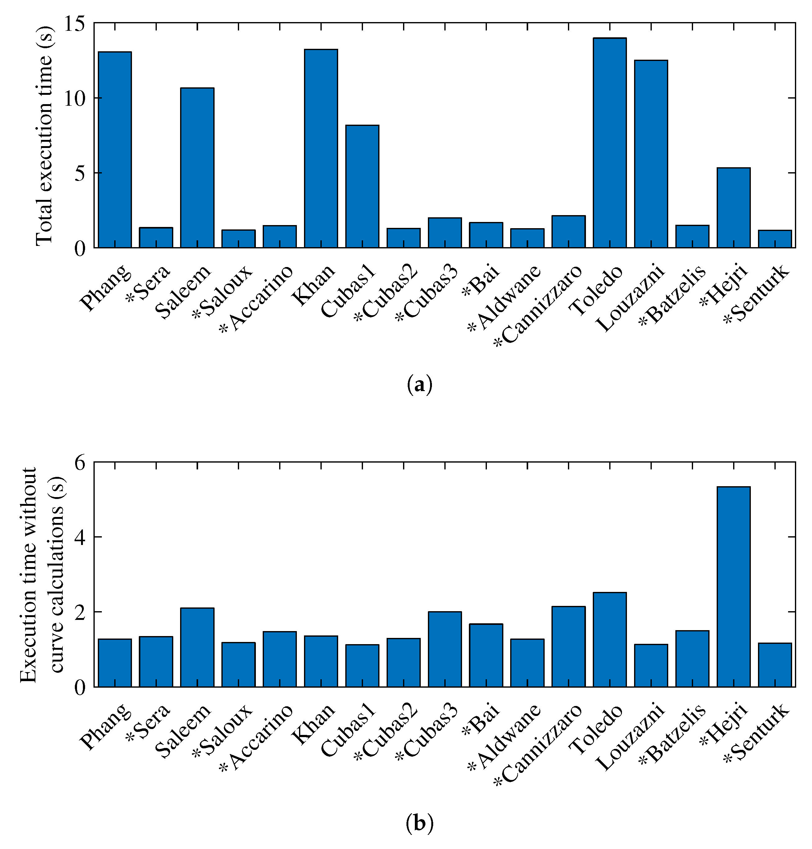
Table 3 shows that for all 1 million curves, the total execution time is between 8–14 s for the methods that involve curve calculations (the ones without an “*”) and 1–2 s for those that rely only on datasheet information, except for Hejri which exhibits a 5.4 s total time due to the large number of calculations with complex numbers. A graphical illustration of this performance is given in Figure 6a: the increased cost of Phang, Khan, Cubas1, Toledo and Louzazni is due to the extraction of the slopes at SC and OC via linear fitting on several samples (see Appendix B), while for Saleem is because it has to identify two additional operating points in the curve apart from the inputs SC, OC, and MPP. The execution time is not affected by the PV technology or operating conditions.

If the curve calculations cost is excluded (core time), Table 3 and Figure 6b show that the remaining time is much lower in the range of 1–2 s, the same as for the only-datasheet methods. This is because the non-iterative methods involve very few and simple equations, whose evaluation cost is comparably less than the curve calculations. If the additional curve-related data are provided as inputs, calculated beforehand, the last column in Table 3 should be used when assessing the computational performance.

In any case, the times recorded for all methods (with and without the curve calculations cost) are as low as a few microseconds per curve, which is several orders of magnitude less than the numerical or optimization counterparts. As an indication of this huge difference, the iterative method given in [34] was evaluated on the same 1-million dataset using a 20-machine computer cluster, whereas here a common PC was able to complete this task in only a few seconds collectively for all methods.

4.2. The Methods that Rely Only on Datasheet Information

Relying only on datasheet information is commonly considered a desirable feature for a parameter extraction method [19,27,36]; the input data are usually the voltage and current at the SC, OC, MPP and possibly the temperature coefficients (see Table 1). This information is readily available at STC and there is no need for additional measurements, which renders the respective methods more easily and universally applicable. In this section, these techniques are reexamined separately to facilitate selection when there are limitations on the input data.

Table 5. Performance of the methods that rely solely on datasheet information.

	Accuracy (RMSE)				Robustness		Complexity
	Absolute (A)		Normalized (%)
Method	Mean	Max	Mean	Max	Irregularities	Failures	Total Time (s)
* Sera	0.026	2.471	0.74	49.6	794,670	52	1.3
* Saloux	0.029	1.271	0.79	25.5	2	0	1.2
* Accarino	0.034	0.880	1.09	17.7	2804	25	1.5
* Cubas2	0.026	2.433	0.64	48.8	626,150	53	1.3
* Cubas3	0.024	0.430	0.83	13.0	1878	224	2.0
* Bai	0.032	2.544	0.93	51.1	6390	37	1.7
* Aldwane	0.021	1.032	0.59	20.7	416,650	29	1.3
* Cannizzaro	0.013	0.431	0.39	11.3	100	28	2.1
* Batzelis	0.028	0.932	0.87	18.7	412	0	1.5
* Hejri	0.231	6.761	7.21	129.4	794,670	14,057	5.4
* Senturk	0.034	1.285	1.09	25.8	27,847	0	1.2

The asterisk “*” denotes methods that rely only on datasheet information. Bold font indicates the lowest value in the respective column.

shows the performance of these methods; the main conclusions derived in the previous section do not change, but the best candidates in some assessment criteria are different. In terms of accuracy, the Cannizzaro technique is now the most preferable, yielding the lowest both mean and max errors (along with Cubas3 for the max absolute RMSE). It is worth noting that the four methods that never exceed the 1 A (20%) RMSE (Accarino, Cubas3, Cannizzaro, and Batzelis) are all included in this table, which indicates that the entire I-V curve is not mandatory to achieve good worst-case accuracy. As for the robustness, the methods that yield irregular results in less than 0.1% of the times (Saloux, Cannizzaro, and Batzelis) and the ones that do not fail even once (Saloux, Batzelis, and Senturk) are all of the only-datasheet type (Table 5). Finally, the execution time of all these methods is pretty much the same (except for Hejri as explained in Section 4.1.3), the small differences being attributed to the number of calculation steps. It is worth noting that the methods that employ the Lambert W function (Accarino, Cubas3, Cannizzaro, and Batzelis) do not exhibit any noticeable overhead in the computational time, due to the approximation formulae used for the principal and lower branches (see Appendix A).

In conclusion, these results show that the most favorable options in terms of worst-case accuracy, irregularities, failures, and execution time are methods that do not require additional measurements apart from the ones available in the PV module datasheet. However, when the average accuracy is the main assessment criterion, the Toledo method that needs extra information, yields significantly lower errors.

4.3. The Methods that Require the SC Slope as Input Data

The extraction of the slope at SC and OC is a challenging task, especially when the I-V curve contains measurement noise or exhibits other types of distortions. Erroneous identification of the slopes has a critical impact on the methods that rely on this data; a factor that affects this identification is the fitting range, i.e., the part of the curve used for linear fitting to calculate the slope (see Appendix B). To investigate this dependence, the performance of Phang, Khan, Cubas1, Toledo and Louzazni are shown in

Table 6. Performance of the methods that require the SC slope as input data.

		Accuracy (RMSE)				Robustness		Complexity
	Fitting	Absolute (A)		Normalized (%)				Execution Time (s)
Method	Range	Mean	Max	Mean	Max	Irregularities	Failures	Total	Core
Phang	0–10%	0.016	4.210	0.38	69.4	387,440	9952	13.1	1.3
	0–50%	0.013	4.226	0.31	69.7	292,530	9613	15.1	1.4
Khan	0–10%	0.043	4.201	1.19	69.3	511,210	8242	13.2	1.4
	0–50%	0.062	4.199	1.70	69.2	490,640	8207	14.4	1.4
Cubas1	0–10%	0.011	2.445	0.36	49.1	529,530	2445	8.2	1.1
	0–50%	0.013	2.074	0.32	41.7	330,470	1591	9.3	1.2
Toledo	0–10%	0.007	1.119	0.20	97.7	451,220	392	14.0	2.5
	0–50%	0.006	2.528	0.17	51.2	315,110	456	16.4	2.8
Louzazni	0–10%	0.122	1.449	3.43	27.0	64,194	30,612	12.5	1.1
	0–50%	0.111	1.508	3.18	43.9	33,147	25,429	14.2	1.3

Bold font indicates the lowest value in the respective column.

for two different SC slope fitting ranges: 0–10% of $V_{oc}$ (short range—used in the previous sections) and 0–50% of $V_{oc}$ (long range). The former option is theoretically closer to the definition of the SC slope (samples on the SC region) and thus it is used throughout the paper, while the latter is less prone to local distortions and irregularities in the I-V curve.

Apparently, the results in all six performance indicators do not fundamentally differ between the two ranges. No clear conclusion can be extracted on the accuracy, each method being affected differently by the larger range, either positively or negatively, without any noteworthy deviations. Exception to this observation is Toledo, which seems to slightly gain from the larger range in terms of average (absolute and normalized) accuracy, but at the cost of much higher absolute RMSE, although the normalized RMSE is reduced. On the other hand, a clear trend is evident in the robustness: all methods exhibit less irregularities and failures at the larger range, which validates the claim that a larger slope extraction range entails better robustness. It is worth noting that Toledo fails the lowest number of times among the slope-relying methods, which is comparable to some of the only-datasheet counterparts (see also Table 5). The execution times recorded are slightly higher in the larger range case, as expected, due to the higher number of samples to be processed. In fact, the conclusion of this investigation is that a larger fitting range for the extraction of the SC slope handles better distorted I-V curves but does not address the problem and may affect the accuracy.

5. Conclusions

This paper performs a rigorous review and assessment of the available non-iterative methods to extract the single-diode PV model parameters. A total of 17 methods are reviewed, implemented, and compared on a dataset of about 1 million I-V curves of six different PV technologies. Some of the main conclusion are:

• Although the simple single-diode model is not the best option for thin-film technologies and low-irradiance measurements, some of the methods perform universally quite decently
• The non-iterative methods are one order of magnitude less accurate than the state-of-the-art numerical counterparts, but require less input data and are much more computationally efficient
• Toledo exhibits the best average accuracy in all PV technologies, whereas the highest worst-case accuracy is brought by a different method in each module type
• Several methods yield negative parameter values (and complex in Hejri) in almost half of the scenarios; this may be acceptable for some applications
• The fewer irregularities are found in Saloux, Cannizzaro, and Batzelis
• Some methods suffer from execution failures quite often, mainly in the HIT and CIGS technologies
• Successful execution is always guaranteed by Accarino, Batzelis, and Senturk
• A major reason for failure is the SC slope extraction due to distorted I-V curve
• A large fitting range for the slope extraction improves slightly the robustness of the slope-relying methods, but has an unpredictable impact on the accuracy
• The calculation times are in the range of microseconds per curve, the higher times observed in the methods that perform calculations on the I-V curve measurements, mainly slope extraction; if this overhead is excluded, the execution time of most methods is quite similar
• The methods that rely only on datasheet information provide the best universal performance in all aspects apart from the average accuracy
• The Lambert W function is related to excellent performance (Accarino, Cubas3, Cannizzaro and Batzelis)

To facilitate selection of the most appropriate method for universal application to all PV technologies,

Table 7. Methods with the best universal performance regarding constraints.

Metric	Constraints
	None	Only-Datasheet	<0.1% Irregularities	No Failures
Mean absolute RMSE	Toledo	Cannizzaro	Cannizzaro	Batzelis
Max absolute RMSE	Cannizzaro, Cubas3	Cannizzaro, Cubas3	Cannizzaro	Batzelis
Mean normalized RMSE	Toledo	Cannizzaro	Cannizzaro	Saloux
Max normalized RMSE	Cannizzaro	Cannizzaro	Cannizzaro	Batzelis
Irregularities	Saloux	Saloux	Saloux	Saloux
Total time	Saloux	Saloux	Saloux	Saloux

below shows the best candidates according to six metrics and accounting for different constraints. Toledo should be selected if focusing on average accuracy and there is access to additional information apart from the datasheet, otherwise the Cannizaro method is more appropriate. When irregular parameters are acceptable to some extent (less than 0.1% of the cases), Cannizzaro yields the best accuracy in terms of both mean and max errors. However, if the execution failures are not acceptable, the Batzelis alternative should be selected instead. Finally, Saloux exhibits always the fewest parameter irregularities and the least execution time, but at the cost of moderate accuracy.

References

- Jordehi, A.R. Parameter estimation of solar photovoltaic (PV) cells: A review. Renew. Sustain. Energy Rev. 2016, 61, 354–371. [Google Scholar] [CrossRef]
- De Soto, W.; Klein, S.; Beckman, W. Improvement and validation of a model for photovoltaic array performance. Sol. Energy 2006, 80, 78–88. [Google Scholar] [CrossRef] [Green Version]
- Laudani, A.; Riganti Fulginei, F.; Salvini, A. Identification of the one-diode model for photovoltaic modules from datasheet values. Sol. Energy 2014, 108, 432–446. [Google Scholar] [CrossRef]
- Laudani, A.; Mancilla-David, F.; Riganti-Fulginei, F.; Salvini, A. Reduced-form of the photovoltaic five-parameter model for efficient computation of parameters. Sol. Energy 2013, 97, 122–127. [Google Scholar] [CrossRef]
- ALQahtani, A.H. A simplified and accurate photovoltaic module parameters extraction approach using matlab. In Proceedings of the 2012 IEEE International Symposium on Industrial Electronics, Hangzhou, China, 28–31 May 2012; pp. 1748–1753. [Google Scholar]
- Lineykin, S.; Averbukh, M.; Kuperman, A. An improved approach to extract the single-diode equivalent circuit parameters of a photovoltaic cell/panel. Renew. Sustain. Energy Rev. 2014, 30, 282–289. [Google Scholar] [CrossRef]
- Villalva, M.; Gazoli, J.; Filho, E. Comprehensive approach to modeling and simulation of photovoltaic arrays. IEEE Trans. Power Electron. 2009, 24, 1198–1208. [Google Scholar] [CrossRef]
- Chenni, R.; Makhlouf, M.; Kerbache, T.; Bouzid, A. A detailed modeling method for photovoltaic cells. Energy 2007, 32, 1724–1730. [Google Scholar] [CrossRef]
- Carrero, C.; Ramírez, D.; Rodríguez, J.; Platero, C. Accurate and fast convergence method for parameter estimation of PV generators based on three main points of the I–V curve. Renew. Energy 2011, 36, 2972–2977. [Google Scholar] [CrossRef]
- Mahmoud, Y.A.; Xiao, W.; Zeineldin, H.H. A parameterization approach for enhancing PV model accuracy. IEEE Trans. Ind. Electron. 2013, 60, 5708–5716. [Google Scholar] [CrossRef]
- Cannizzaro, S.; Di Piazza, M.C.; Luna, M.; Vitale, G. Generalized classification of PV modules by simplified single-diode models. In Proceedings of the 2014 IEEE 23rd International Symposium on Industrial Electronics (ISIE), Istanbul, Turkey, 1–4 June 2014; pp. 2266–2273. [Google Scholar]
- Accarino, J.; Petrone, G.; Ramos-Paja, C.A.; Spagnuolo, G. Symbolic algebra for the calculation of the series and parallel resistances in PV module model. In Proceedings of the 2013 International Conference on Clean Electrical Power (ICCEP), Alghero, Italy, 11–13 June 2013; pp. 62–66. [Google Scholar]
- Nassar-eddine, I.; Obbadi, A.; Errami, Y.; El fajri, A.; Agunaou, M. Parameter estimation of photovoltaic modules using iterative method and the Lambert W function: A comparative study. Energy Convers. Manag. 2016, 119, 37–48. [Google Scholar] [CrossRef]
- Phang, J.C.H.; Chan, D.S.H.; Phillips, J.R. Accurate analytical method for the extraction of solar cell model paramaters. Electron. Lett. 1984, 20, 406–408. [Google Scholar] [CrossRef]
- Sera, D.; Teodorescu, R.; Rodriguez, P. Photovoltaic module diagnostics by series resistance monitoring and temperature and rated power estimation. In Proceedings of the 2008 34th Annual Conference of IEEE Industrial Electronics, Orlando, FL, USA, 10–13 November 2008; pp. 2195–2199. [Google Scholar]
- Saleem, H.; Karmalkar, S. An analytical method to extract the physical parameters of a solar cell from four points on the illuminated J-V curve. IEEE Electron Device Lett. 2009, 30, 349–352. [Google Scholar] [CrossRef]
- Saloux, E.; Teyssedou, A.; Sorin, M. Explicit model of photovoltaic panels to determine voltages and currents at the maximum power point. Sol. Energy 2011, 85, 713–722. [Google Scholar] [CrossRef]
- Khan, F.; Baek, S.H.; Park, Y.; Kim, J.H. Extraction of diode parameters of silicon solar cells under high illumination conditions. Energy Convers. Manag. 2013, 76, 421–429. [Google Scholar] [CrossRef]
- Cubas, J.; Pindado, S.; Victoria, M. On the analytical approach for modeling photovoltaic systems behavior. J. Power Sources 2014, 247, 467–474. [Google Scholar] [CrossRef] [Green Version]
- Bai, J.; Liu, S.; Hao, Y.; Zhang, Z.; Jiang, M.; Zhang, Y. Development of a new compound method to extract the five parameters of PV modules. Energy Convers. Manag. 2014, 79, 294–303. [Google Scholar] [CrossRef]
- Aldwane, B. Modeling, simulation and parameters estimation for Photovoltaic module. In Proceedings of the 2014 1st International Conference on Green Energy ICGE 2014, Sfax, Tunisia, 25–27 March 2014; pp. 101–106. [Google Scholar]
- Cannizzaro, S.; Di Piazza, M.C.; Luna, M.; Vitale, G. PVID: An interactive Matlab application for parameter identification of complete and simplified single-diode PV models. In Proceedings of the 2014 IEEE 15th Workshop on Control and Modeling for Power Electronics (COMPEL), Santander, Spain, 22–25 June 2014. [Google Scholar]
- Toledo, F.; Blanes, J.M. Geometric properties of the single-diode photovoltaic model and a new very simple method for parameters extraction. Renew. Energy 2014, 72, 125–133. [Google Scholar] [CrossRef]
- Louzazni, M.; Aroudam, E.H. An analytical mathematical modeling to extract the parameters of solar cell from implicit equation to explicit form. Appl. Sol. Energy 2015, 51, 165–171. [Google Scholar] [CrossRef]
- Batzelis, E.I.; Papathanassiou, S.A. A method for the analytical extraction of the single-diode PV model parameters. IEEE Trans. Sustain. Energy 2016, 7, 504–512. [Google Scholar] [CrossRef]
- Hejri, M.; Mokhtari, H.; Azizian, M.R.; Söder, L. An analytical-numerical approach for parameter determination of a five-parameter single-diode model of photovoltaic cells and modules. Int. J. Sustain. Energy 2016, 35, 396–410. [Google Scholar] [CrossRef]
- Senturk, A.; Eke, R. A new method to simulate photovoltaic performance of crystalline silicon photovoltaic modules based on datasheet values. Renew. Energy 2017, 103, 58–69. [Google Scholar] [CrossRef]
- Murtaza, A.; Munir, U.; Chiaberge, M.; Di Leo, P.; Spertino, F. Variable Parameters for a Single Exponential Model of Photovoltaic Modules in Crystalline-Silicon. Energies 2018, 11, 2138. [Google Scholar] [CrossRef]
- Kumar, M.; Kumar, A. An efficient parameters extraction technique of photovoltaic models for performance assessment. Sol. Energy 2017, 158, 192–206. [Google Scholar] [CrossRef]
- Ibrahim, H.; Anani, N. Evaluation of Analytical Methods for Parameter Extraction of PV modules. Energy Procedia 2017, 134, 69–78. [Google Scholar] [CrossRef]
- Xiong, G.; Zhang, J.; Yuan, X.; Shi, D.; He, Y.; Yao, G. Parameter extraction of solar photovoltaic models by means of a hybrid differential evolution with whale optimization algorithm. Sol. Energy 2018, 176, 742–761. [Google Scholar] [CrossRef]
- Soon, J.J.; Low, K.S. Photovoltaic model identification using particle swarm optimization with inverse barrier constraint. IEEE Trans. Power Electron. 2012, 27, 3975–3983. [Google Scholar] [CrossRef]
- Askarzadeh, A.; Dos Santos Coelho, L. Determination of photovoltaic modules parameters at different operating conditions using a novel bird mating optimizer approach. Energy Convers. Manag. 2015, 89, 608–614. [Google Scholar] [CrossRef]
- Toledo, F.J.; Blanes, J.M.; Galiano, V. Two-Step Linear Least-Squares Method For Photovoltaic Single-Diode Model Parameters Extraction. IEEE Trans. Ind. Electron. 2018, 65, 6301–6308. [Google Scholar] [CrossRef]
- Lim, L.H.I.; Ye, Z.; Ye, J.; Yang, D.; Du, H. A linear identification of diode models from single I-V characteristics of PV panels. IEEE Trans. Ind. Electron. 2015, 62, 4181–4193. [Google Scholar] [CrossRef]
- Ciulla, G.; Lo Brano, V.; Di Dio, V.; Cipriani, G. A comparison of different one-diode models for the representation of I–V characteristic of a PV cell. Renew. Sustain. Energy Rev. 2014, 32, 684–696. [Google Scholar] [CrossRef]
- Chin, V.J.; Salam, Z.; Ishaque, K. Cell modelling and model parameters estimation techniques for photovoltaic simulator application: A review. Appl. Energy 2015, 154, 500–519. [Google Scholar] [CrossRef]
- Humada, A.M.; Hojabri, M.; Mekhilef, S.; Hamada, H.M. Solar cell parameters extraction based on single and double-diode models: A review. Renew. Sustain. Energy Rev. 2016, 56, 494–509. [Google Scholar] [CrossRef] [Green Version]
- Boutana, N.; Mellit, A.; Lughi, V.; Massi Pavan, A. Assessment of implicit and explicit models for different photovoltaic modules technologies. Energy 2017, 122, 128–143. [Google Scholar] [CrossRef]
- Piazza, M.C.D.; Luna, M.; Petrone, G.; Spagnuolo, G. Translation of the Single-Diode PV Model Parameters Identified by Using Explicit Formulas. IEEE J. Photovolt. 2017, 7, 1009–1016. [Google Scholar] [CrossRef]
- Peñaranda Chenche, L.E.; Hernandez Mendoza, O.S.; Bandarra Filho, E.P. Comparison of four methods for parameter estimation of mono- and multi-junction photovoltaic devices using experimental data. Renew. Sustain. Energy Rev. 2018, 81, 2823–2838. [Google Scholar] [CrossRef]
- Marion, B.; Anderberg, A.; Deline, C.; del Cueto, J.; Muller, M.; Perrin, G.; Rodriguez, J.; Rummel, S.; Silverman, T.J.; Vignola, F.; et al. New data set for validating PV module performance models. In Proceedings of the 2014 IEEE 40th Photovoltaic Specialist Conference (PVSC), Denver, CO, USA,, 8–13 June 2014; pp. 1362–1366. [Google Scholar]
- Batzelis, E.I. Simple PV performance equations theoretically well-founded on the single-diode model. IEEE J. Photovolt. 2017, 7, 1400–1409. [Google Scholar] [CrossRef]
- Karatepe, E.; Boztepe, M.; Çolak, M. Development of a suitable model for characterizing photovoltaic arrays with shaded solar cells. Sol. Energy 2007, 81, 977–992. [Google Scholar] [CrossRef]
- Quaschning, V.; Hanitsch, R. Numerical simulation of current-voltage characteristics of photovoltaic systems with shaded solar cells. Sol. Energy 1996, 56, 513–520. [Google Scholar] [CrossRef]
- Pandey, P.K.; Sandhu, K. Multi diode modelling of PV cell. In Proceedings of the 2014 IEEE 6th India International Conference on Power Electronics (IICPE), Kurukshetra, India, 8–10 December 2014. [Google Scholar]
- Kawamura, H.; Naka, K.; Yonekura, N.; Yamanaka, S.; Kawamura, H.; Ohno, H.; Naito, K. Simulation of I–V characteristics of a PV module with shaded PV cells. Sol. Energy Mater. Sol. Cells 2003, 75, 613–621. [Google Scholar] [CrossRef]
- Merten, J.; Asensi, J.; Voz, C.; Shah, A.; Platz, R.; Andreu, J. Improved equivalent circuit and analytical model for amorphous silicon solar cells and modules. IEEE Trans. Electron Devices 1998, 45, 423–429. [Google Scholar] [CrossRef] [Green Version]
- Abbassi, A.; Gammoudi, R.; Ali Dami, M.; Hasnaoui, O.; Jemli, M. An improved single-diode model parameters extraction at different operating conditions with a view to modeling a photovoltaic generator: A comparative study. Sol. Energy 2017, 155, 478–489. [Google Scholar] [CrossRef]
- Celik, A.N.; Acikgoz, N. Modelling and experimental verification of the operating current of mono-crystalline photovoltaic modules using four- and five-parameter models. Appl. Energy 2007, 84, 1–15. [Google Scholar] [CrossRef]
- Hejri, M.; Mokhtari, H.; Azizian, M.R.; Ghandhari, M.; Soder, L. On the parameter extraction of a five-parameter double-diode model of photovoltaic cells and modules. IEEE J. Photovolt. 2014, 4, 915–923. [Google Scholar] [CrossRef]
- Chouder, A.; Silvestre, S.; Sadaoui, N.; Rahmani, L. Modeling and simulation of a grid connected PV system based on the evaluation of main PV module parameters. Simul. Model. Pract. Theory 2012, 20, 46–58. [Google Scholar] [CrossRef]
- Kou, Q.; Klein, S.; Beckman, W. A method for estimating the long-term performance of direct-coupled PV pumping systems. Sol. Energy 1998, 64, 33–40. [Google Scholar] [CrossRef]
- Tian, H.; Mancilla-David, F.; Ellis, K.; Muljadi, E.; Jenkins, P. A cell-to-module-to-array detailed model for photovoltaic panels. Sol. Energy 2012, 86, 2695–2706. [Google Scholar] [CrossRef]
- Khezzar, R.; Zereg, M.; Khezzar, A. Modeling improvement of the four parameter model for photovoltaic modules. Sol. Energy 2014, 110, 452–462. [Google Scholar] [CrossRef]
- Cubas, J.; Pindado, S.; de Manuel, C. Explicit expressions for solar panel equivalent circuit parameters based on analytical formulation and the Lambert W-function. Energies 2014, 7, 4098–4115. [Google Scholar] [CrossRef]
- Petrone, G.; Ramos-Paja, C.A.; Spagnuolo, G. Photovoltaic Sources Modeling, 1st ed.; Wiley-IEEE Press: Hoboken, NJ, USA, 2017; p. 208. [Google Scholar]
- Mahmoud, Y.; El-Saadany, E.F. Fast power-peaks estimator for partially shaded PV systems. IEEE Trans. Energy Convers. 2016, 31, 206–217. [Google Scholar] [CrossRef]
- Anderson, A.J. Photovoltaic Translation Equations: A New Approach; National Renewable Energy Laboratory: Golden, CO, USA, 1996. [Google Scholar]
- Chan, D.S.H.; Phillips, J.R.; Phang, J.C.H. A comparative study of extraction methods for solar cell model parameters. Solid State Electron. 1986, 29, 329–337. [Google Scholar] [CrossRef]
- Chan, D.S.H.; Phang, J.C.H. Analytical methods for the extraction of solar-cell single- and double-diode model parameters from I-V characteristics. IEEE Trans. Electron Devices 1987, ED, 286–293. [Google Scholar] [CrossRef]
- Hadj Arab, A.; Chenlo, F.; Benghanem, M. Loss-of-load probability of photovoltaic water pumping systems. Sol. Energy 2004, 76, 713–723. [Google Scholar] [CrossRef]
- Orioli, A.; Di Gangi, A. A procedure to calculate the five-parameter model of crystalline silicon photovoltaic modules on the basis of the tabular performance data. Appl. Energy 2013, 102, 1160–1177. [Google Scholar] [CrossRef] [Green Version]
- Technical Guideline. Generic Solar Photovoltaic System Dynamic Simulation Model Specification; Sandia National Laboratorie: Livermore, CA, USA, 2013. [Google Scholar]
- Corless, R.M.; Gonnet, G.H.; Hare, D.E.G.; Jeffrey, D.J.; Knuth, D.E. On the Lambert W function. Adv. Comput. Math. 1996, 5, 329–359. [Google Scholar] [CrossRef]
- Batzelis, E.I.; Routsolias, I.A.; Papathanassiou, S.A. An explicit PV string model based on the Lambert W function and simplified MPP expressions for operation under partial shading. IEEE Trans. Sustain. Energy 2014, 5, 301–312. [Google Scholar] [CrossRef]
- Barry, D.; Parlange, J.Y.; Sander, G.; Sivaplan, M. A class of exact solutions for Richards’ equation. J. Hydrol. 1993, 142, 29–46. [Google Scholar] [CrossRef]
- Xiao, W.; Lind, M.; Dunford, W.; Capel, A. Real-time identification of optimal operating points in photovoltaic power systems. IEEE Trans. Ind. Electron. 2006, 53, 1017–1026. [Google Scholar] [CrossRef]
Figure 1.
Electrical equivalent circuit of the single-diode PV model.
Figure 2.
Typical I-V characteristic curve of a PV module in the first quadrant.
Figure 3.
Histograms of (a) irradiance and (b) temperature distribution of the study-case dataset.
Figure 4.
Accuracy of the 17 methods. (a) Cumulative mean normalized RMSE and (b) max normalized RMSE for the various PV technologies.
Figure 5.
Robustness of the 17 methods. (a) Number and (b) types of irregularities. (c) Execution failures.
Figure 6.
Computational cost of the 17 methods. (a) Total execution time. (b) Execution time excluding curve calculations.