Maximizing the Economic Benefits of a Grid-Tied Microgrid Using Solar-Wind Complementarity


1
Electrical Engineering Department, Lahore University of Management Sciences (LUMS), Lahore 54792, Pakistan
2
Engineering Product Development, Singapore University of Technology and Design (SUTD), 8 Somapah Road, Singapore 487372, Singapore
3
Department of Electrical and Computer Engineering, Curtin University, Perth, WA 6845, Australia
*
Author to whom correspondence should be addressed.
Energies 2019, 12(3), 395; https://doi.org/10.3390/en12030395
Submission received: 29 December 2018
/
Revised: 19 January 2019
/
Accepted: 25 January 2019
/
Published: 27 January 2019
(This article belongs to the Section F: Electrical Engineering)
Abstract
:The increasing use of intermittent, renewable energy sources (RESs) for electricity generation in microgrids (MGs) requires efficient strategies for reliable and economic operation. Complementarity between RESs provides good prospects for integrating several local energy sources and reducing the costs of MG setup and operations. This paper presents a framework for maximizing the economic benefits of a grid-tied MG by exploiting the spatial and temporal complementarity between solar and wind energies (solar-wind complementarity). The proposed framework considers the cost of energy production from different RESs and the cost of bi-directional energy exchange with the main grid. For a given RES mix, a minimum system power loss (SPL) threshold can also be determined. However, at this SPL threshold, MG energy exchange cost is not always minimized. The framework determines the optimized SPL value (above the threshold) at which MG energy exchange cost gets minimized. Through this framework, MG operator can decide appropriate RES mix and can achieve various tradeoffs according to the energy production cost, solar-wind complementarity of the site and its required economic objectives.
1. Introduction
Traditional power systems are witnessing significant changes due to ever increasing penetration of distributed renewable energy sources (RESs) [1]. Solar and wind are the two most widely used RESs and both of them are inherently intermittent. The integration of such RES in power systems requires careful planning, novel system architectures, and fallback options to maintain supply-demand balance and power system reliability.
Solar and wind energy are also distributed in nature. Faster integration of these distributed RESs in power systems can be facilitated through microgrids (MG). MGs are localized power grids built to exploit locally available energy sources [2,3,4,5,6,7]. Inclusion of energy storage system (ESS) in MG is a popular strategy to buffer RES variations [8,9,10]. However, despite significant advancements in technology, the cost of ESS still remains quite high. Particularly, large-scale (MWh) ESS tends to be extremely expensive and per MWh, ESS cost can run into several million USD [11]. Tying MG to the main power grid (termed as grid-tied mode) is another convenient method to overcome local supply-demand mismatches. In this grid-tied mode, any shortfall in electricity production could be met by procuring energy from the main grid, while excess energy produced by the RES could also be sold to the main grid. However, to regulate voltage/frequency on the main grid, power system regulators may impose certain limitations on RES intermittency in MGs [12,13,14].
In this context, some RES intermittency in grid-tied MG may be mitigated through careful planning and investments in complementary RES, e.g., solar and wind [15,16,17,18,19]. At several geographical locations, solar irradiance and wind speeds have different (often opposite) variability characteristics. When one RES is producing less power, the other RES is producing more power, and vice versa. The combined power produced by solar and wind RES at such locations has a more steady profile as compared to the power produced by individual RES (solar only or wind only). In addition to the inclusion of complementary RES, the economic viability of MG may be further enhanced by determining the appropriate RES mix, which also indicates the share of each RES in electricity generation, and by reducing the operational costs.
The potential of solar-wind complementarity in maximizing the economic benefit of a grid-tied MG was studied. This problem is challenging because RES mix not only depends on the solar-wind complementarity at MG location but also on the cost of energy production from different RES. Moreover, bi-directional energy exchange with the main grid incurs additional costs for MG. In addition to system power losses (SPL), energy export cost (from MG to grid), energy import cost (from grid to MG), and energy exchange costs also depend on the RES mix.
To this end, a unified framework was developed, which allows the MG operator to take all the relevant factors into account in order to maximize the economic benefits of a grid-tied MG. For a given solar-wind complementarity value, levelized costs of solar and wind RES, and energy import and export costs, RES mix is varied in the proposed framework. For each value of RES mix, the framework determines the energy exchange cost. Energy exchange cost also includes the cost due to system power loss (SPL). The framework determines the minimum SPL threshold at which the amount of energy exchanged is minimized. However, at this SPL threshold, MG energy exchange cost is not always minimized due to differences in energy import and export costs. Moreover, RES mix also turns out to be different according to solar-wind complementarity of the site, energy production costs and energy import and export cost variations. The optimization problems in this framework are non-convex, which are solved using particle swarm optimization (PSO) and exterior penalty function (EPF) techniques to obtain efficient solutions. The application of the proposed framework for a grid-tied MG is demonstrated by modeling MG as a balanced IEEE 33-bus system, at four different locations in Ireland each with a different solar-wind complementarity value. RES mix is determined at each location and interesting observations are provided. MG operator can use this unified framework to maximize its economic benefits by deciding appropriate RES mix, which minimizes the energy exchange costs as well as the energy production costs.
Literature Review
The literature addressing the economic gains of a MG that is equipped with PV units and wind turbines can be found in [20,21,22,23,24,25,26]. The authors in [20] attempted to minimize the operational and maintenance costs of a MG by utilizing the demand side flexibility. The proposed optimization method uses mixed integer linear programming to solve the scheduling problem. The research conducted in [21] also makes use of demand side flexibility to schedule the loads such that the electricity cost is minimized. The proposed problem is solved using centralized algorithms. Similarly, an economic dispatch strategy for various types of distributed generators to minimize the power generation costs of a grid-tied MG is proposed in [22]. However, to compensate for the intermittent power generated by RESs in autonomous conditions, non-renewable energy based power generators are deployed. The proposed economic dispatch problem is solved through direct search method (DSM). The operational cost of a MG is minimized through a dispatch strategy of fuel cell and natural gas based micro turbine in [23]. The proposed strategy is solved through particle swarm optimization (PSO) and tested on IEEE 33-bus system. An operational scheme to schedule the diesel generators that aims to minimize the day-ahead aggregate cost of electricity, while offsetting the intermittency of RESs, is proposed in [24]. The costs of operation, emission, and network losses are accommodated in the aggregate cost. To solve the cost minimization problem, the authors use modified differential evolution algorithm and test their proposed strategy on IEEE 33-bus system. The research conducted in [25] also attempts to maximize the economic gains of a microgrid, but the power generators in this case include a dispatchable diesel generator along with ESS to smooth out solar and wind variations. In [26], a multi-objective optimization model of a MG consisting of electric vehicles (EVs), diesel generators and RESs has been proposed. The objectives of this study includes minimization of operational costs, reduction of power fluctuations, and minimization of net load of MG. The authors solved this problem through multi-objective PSO.
Although the recent approaches are able to improve the economic viability of a MG, they suffer from some drawbacks. A careful review of these papers suggests that these studies rely on backup ESS or a diesel generator to account for the intermittency of solar and wind RESs. The inclusion of ESS introduces the additional charge/discharge scheduling and capacity sizing problem. In addition, the battery replacement cost, number of charge/discharge cycles, stochastic nature of the arrival of EVs (i.e., driving patterns) and the initial state of charge complicates the problem further. Furthermore, power generation by means of burning a fossil fuel raises environmental concerns and introduces additional fuel cost and penalty associated with environmental degradation. From the technical perspective, the existing studies neglect the power losses that occur due to resistance in power transmission lines [27,28]. This constraint has a substantial impact on the operational cost of a grid-tied MG as it limits the number of power transactions occurring with the main grid due to physical parameters of the system.
Several studies have been conducted to evaluate solar-wind complementarity in various regions [16,17,18,19,29,30,31,32,33,34,35]. In [16], the authors exploit the solar-wind complementarity and hydropower along the downstream areas of Yalong River with the objective to stabilize the power produced. However, this study utilizes the flexibility of the hydro-power units to mitigate the randomness in solar and wind RES. The authors in [17] also discuss the complementarity between the outputs of renewable energy sources and their proposed model utilizes the variable characteristics between the power sources and the load. Based on the power patterns of solar and wind RES in four different locations of Hong Kong, the authors in [18] propose a theoretical framework to assess the investment cost of solar photovoltaic (PV) units and wind turbines. The study in [19] investigates the key features of solar-wind complementarity in Britain for energy balancing. The research conducted in [29] aims to minimize the power losses in a distribution power system by using spatial and temporal complementarity of solar and wind energy sources. Likewise, the authors in [30] exploit temporal complementarity between RESs to reduce the net variability between supply and demand, along with investment costs of solar and wind energy sources in MGs. Similarly, studies in [31,32] assess the temporal solar-wind complementarity across Europe by means of correlation coefficients. However, neither study includes the modeling of power systems or load profiles for the evaluation. In contrast, the work conducted in [33] provides an analysis of the influence of the complementary characteristics between RES, load and grid on the energy reserve requirements and in [34], a study of the complementarity of RES with the load demand is presented. However, an important consideration in these studies is that they focus on the complementarity between the resource and the load demand rather than the complementarity between the RESs. Complementarity between RESs has also been exploited in a hybrid wind–solar system integrated with battery storage to match the load demand at a specific location in [35].
The existing studies lack a holistic structure to analyze the influence of solar-wind complementarity on the economic gains of a grid-tied MG. This paper provides such a unified framework, while taking into account all the relevant factors and costs. Through the proposed framework, MG may also achieve various tradeoffs depending on its required economic objectives.
The rest of the paper is organized as follows. In Section 2, the MG Model used in this work is presented, followed by a discussion on the solar-wind complementarity. In Section 3, the proposed framework is formulated and the solution techniques are presented. In Section 4, the benefits of the proposed framework are verified with the help of numerical study. The paper is concluded in Section 5.
2. MG Model and Solar-Wind Complementarity
This section presents a simplified grid-tied MG Model and describes solar-wind complementarity.
2.1. MG Model
For power flow analysis, consider the balanced MG Model shown in Figure 1. Under balanced conditions, MG network can be represented by a single phase equivalent model [36]. The MG is assumed to have nodes which are indexed by . At nodes, RES (solar, wind or both) could be installed. All nodes are assumed to be closely located with the same solar-wind complementarity value in the network. In addition, MG is tied to the power grid at the point of common coupling (PCC) through which bi-directional power exchanges occur. At ith node in MG, load demand could be fulfilled through power injections made by local RES and power imported from the grid. The net active and reactive power injections occurring at node i can be represented by the following set of recursive equations [1],
At node , the instantaneous active power is given by . It should be noted that in this model the value of means there is no local RES at node i. Similarly, the value of indicates the presence of a local RES (solar, wind or both) at node i. In this paper, it is assumed that the values of are already fixed.
Assuming both solar and wind RES, can be expressed as,
The value of means only wind turbines are installed at node i, while means that only solar PV units are installed at node i in the MG. Any other value () indicates RES mix consisting of some solar and some wind RES at node i. Please note that the value of is not a function of t and this value is fixed during the planning stage of the MG. In addition, all nodes in MG are closely located such that the value of solar-wind complementarity is the same. With this assumption, . In this paper, is an optimization variable and it is proposed to fix this value according to solar-wind complementarity at MG location and the energy production costs of RES. The impact of RES mix on the power flow and energy exchange costs is also studied.
2.2. Solar-Wind Complementarity
The power generated by a PV unit is modeled as [37],
Similarly, the power generated by a wind turbine [38] is modeled as,
The correlation coefficient between solar and wind capacity factors at some geographical location at time t termed as point complementarity [32] can be computed as,
These values are computed by using daily averages of solar irradiance and wind potentials that are determined for a certain number of days until time t.
Figure 2 shows the average monthly powers produced by solar and wind RES. The variations in generated power are plotted for a 2.0 MW PV unit and a 2.0 MW wind turbine at Location C, which is shown in Figure 3. Average monthly values are used based on the assumption that the correlation between the monthly cumulative powers produced by these RES is a better indicator of seasonal influences. On the other hand, hourly correlation might be greatly affected by the day-night variations of sunlight, and the daily wind profile may not follow the same pattern on a similar day such as in [32]. Significant variations in the individual power profiles of solar and wind RES in different months can be observed. However, when the two outputs are combined, overall variations are significantly eliminated.
Spatial complementarity at a given geographical location is evaluated by time averaging the correlation coefficient between solar and wind capacity factors [31]. More negative values mean higher solar-wind complementarity. Spatial complementarity across different regions of Ireland is shown in Figure 3. The areas inside darker toned blocks have higher solar-wind complementarity as compared to the regions inside lighter toned blocks. The sites labeled as A, B, C and D were chosen for the solar-wind complementarity analysis in this study. More details on finding the complementarity are given in Appendix A. In the rest of the paper, the value of solar-wind complementarity at a specified geographical location where MG is located is denoted by .
3. Proposed Framework and Solution
The objective of the proposed framework is to maximize the economic benefit of a grid-tied MG by determining appropriate RES mix according to solar-wind complementarity of the site and by optimizing the resulting energy exchange costs due to energy variations and power loss in the system. In the proposed setup, energy is produced by multiple RES. Generally, the levelized cost of electricity (LCOE) serves as a tool to analyze the cost effectiveness of different types of RES technologies in terms of their installation and generation costs. LCOE can help in deciding RES mix, i.e., the number of solar and wind RESs in a MG. Moreover, the combined power produced by the RES mix has a direct impact on the energy exchange cost. In this way, capital investment costs and operational costs of a MG are interlinked. Formulating a joint optimization problem to find the best RES mix, which also minimizes the energy exchange cost due to resulting energy variations and power loss in the system is not straightforward.
Figure 4 shows the block diagram of the proposed framework. A flexible, unified framework is developed that can be used to determine appropriate RES mix according to all the relevant factors at MG site. To enable maximum flexibility and considering the fact that the objective is to plan RES mix, while simultaneously considering the impact of RES mix on MG operations, an iterative approach can be adopted. The value of is varied and LCOE of RES mix is computed. Then, for each value of and its corresponding LCOE, the energy production cost of the RES mix is determined. In the determination of energy exchange cost, the overall SPL is included as a separate constraint. A minimum value of SPL exists due to RES mix and system constraints, such as thermal capacity of feeders, etc. [39]. The value of is determined through feasibility analysis of the cost minimization problem. This stage is shown as SPL determination in Figure 4. The next step is to determine the feasible optimized value of SPL at which the energy exchange cost is minimized. Then, the values of , , and are fed to the cost minimization block, where the resulting energy exchange cost is determined. This cost is added to the energy production cost to compute a net cost. The final step in this framework is to determine the optimized RES mix, which is the one that minimizes the net cost.
3.1. Energy Production Cost
LCOE is an effective tool to measure the net competitiveness of different types of RESs [40]. These costs are represented by their net present values, which are aggregated over a period of the lifetime of each source [2]. At a given location, for a given value of , the objective is to determine the energy production cost and the energy exchange cost.
For a given RES mix, LCOE is computed as,
Note that the time step in this formula is one year. It should be noted that the investment cost also depends on the local load demand of a MG.
The average annual energy units produced by the RES mix are determined as,
These units are then converted to total annual energy production cost ($) according to the following formula,
3.2. Energy Exchange Cost
Next, for a given value of , the energy exchange cost is determined. For this purpose, the amount of energy exchanged with the grid is considered at each time interval (could be a minute, hour, etc.) and is denoted as t. The amount of energy exchanged with the grid at any time t can be divided into two separate components,
A subtle point about is that it already incorporates the cost of overall SPL as can be inferred from the power balance constraints in Equations (1) and (2) and from Equation (21). Furthermore, the MG operator is assumed to be the price taker [42].
3.2.1. Energy Exchange Cost Minimization Problem
To determine and optimize the energy exchange cost, the cost minimization problem can be formulated as,
The objective optimization problem in Equation (11) is to minimize the accumulated operational cost of energy exchanges. Equations (1), (2) and (9) are power balance constraints at MG nodes. The SPL at any time t is computed by summing all line losses as, . The constraint in Equation (13) imposes a limit on SPL due to thermal capacity of feeders and Equation (14) restricts the line losses at nodes within an acceptable range. Equations (15) and (16) impose upper limits on the amount of energy export and import in one time slot. Equation (17) constraints the apparent power flowing through the slack bus at any time to its upper limit. Equations (18)–(20) bound the reactive power exchanged with solar and wind RES. Finally, Equation (20) is required for voltage regulation in different MG nodes. Note that, if none of the RES technology is installed at ith node, the respective active power injection at that node becomes zero. Thus, these power injections not only specify the magnitude of power flows but can also model the installation of RES technologies at a given node.
The power loss occurring in node i at time t is represented by active and reactive power injections as [43],
This makes Equations (13) and (14) nonlinear. The cost minimization problem formulated in Equations (11)–(20) is a constrained, non-convex optimization problem. Finding optimal solution of such optimization problems in general is not possible. The next subsection provides an efficient solution of the optimization problem using exterior penalty function and PSO.
3.2.2. Solution of Energy Exchange Cost Minimization Problem
Use of exterior penalty function (EPF) is a well-known tool to convert a constrained optimal power flow problem to an unconstrained problem [44]. In contrast to gradient based optimization methods such as Lagrange multiplier method, penalty function does not introduce any disjunction when considering inequality constraints. It allows a constrained nonlinear problem to be solved using unconstrained programming methods by penalizing the outlier solutions in such a way that an optimal solution is obtained in a robust, efficient way. For the cost minimization problem, the following unconstrained problem can be formulated,
where , , , , , snf represent the inequality constraints defined in Equations (13)–(20). The value of n in depends on the number of constraints and in this case, it varies from 1 to 9.
Due to non-convexity and existence of local minima [45], PSO can be used to determine the solution. PSO is an evolutionary method and these methods are becoming popular in solving problems involving nonlinear power flow equations and in determination of the optimal solution in cost minimization problems involving multiple energy sources [23,46]. One important characteristic of PSO is that it is inherently an unconstrained optimization algorithm and it does not require the objective function and the constraints to be differentiable [47]. PSO generates near to global optimum solutions, which ensures that the chance of getting trapped by a local minimum stays negligible.
The modified problem in Equation (22) and the use of PSO led to the development of Algorithm 1. To implement it, the required data and all limits of power flows and penalty factors are obtained. Then, for each time t, the instantaneous power flows and nodal voltages are observed to compute the power loss to check if it is within the desirable range. If any of the observed system state violates the constraints, then it is penalized. Control variables are selected such that the cost of energy exchange is minimized.
3.2.3. Feasibility of Energy Exchange Cost Minimization Problem
An important consideration of the cost minimization problem relates to the SPL that can be sustained by the MG. To find the minimum value of for which the cost minimization problem remains feasible, an SPL minimization problem can be developed as,
Minimizing the objective function in Equation (23) has the effect of reducing the active power loss and it is subjected to power balancing constraints in Equation (24) and some capacity limitations of the system in Equations (17)–(20). The problem formulated in Equations (23)–(25) can be classified as a constrained non-linear reactive power dispatch problem. Once again, due to non-convexity, this problem is solved by using PSO based algorithm similar to Algorithm 1 but with different control variables, i.e., , , , . The details of this algorithm are skipped to avoid repetitions.
| Algorithm 1: Energy exchange cost minimization. |
 |
3.3. Optimized RES Mix
Algorithm 2 illustrates the process of determining optimized RES mix for each location. At a given location of MG, the average energy potentials of each RES are determined by varying the value of by . For each value of , is computed using Equation (7) r to determine from Equation (8). For the same value of , the solution to optimization problem in Equation (23) results in . Then, the value of is varied in the range, , such that is a reasonably high value in order to ensure the optimal value of energy exchange cost cannot be missed. This step sets the value of in Equation (13). Then, Algorithm 1 is executed to determine the value of . The value of is chosen such that it minimizes the energy exchange cost for a given value of . Finally, the costs, and are accumulated to obtain . The optimized RES mix is the one which results in the minimum value of .
| Algorithm 2: Proposed algorithm to determine optimized RES mix. |
|
4. Case Study
To test the proposed framework, an IEEE 33-bus balanced radial distribution system was used that had been modified to a MG [1,2]. Detailed parameters of this system can be found in [48]. For the simulation purpose, the MG was assumed to have a fixed load demand of 3.7 MW and 2.3 MVAr. Figure 5 shows the modified structure of this bus system. The maximum capacity of this system, , was 100 MVA. The voltage magnitude is limited to [0.9 1.1] per unit. All wind turbines were assumed to have similar characteristics (the same is true for PV units) and the generation capacity of each source was 2.0 MW. Furthermore, only wind turbines were considered for reactive power support. For PV units, it is worth mentioning that an inverter based reactive power compensation at full power output requires the inverters to be sized such that they have larger capacity for the same real power rating of power generation unit. As the inverter cost is associated with its current rating, additional inverter capacity implies higher costs of energy production [49]. For this reason, PV units were assumed to operate at unity power factor [50].
To compute the SPL, the load flow analysis was carried out using MATPOWER 6.0 toolbox. The PSO parameters were arbitrarily selected for simulations, which included 100 iterations, inertia weight in the range [0.4 0.9], acceleration constant of 2.05 and a swarm size of 50. Further, all penalty factors were assumed to be equal with magnitude, and the constriction factor was chosen to be 0.729 [51].
For validating the effectiveness of the proposed approach, various system configurations were analyzed. As illustrated by Table 1, the system configurations were classified into three cases. In Case-I, , i.e., only PV units were installed at bus 18, 32 and 33. The choice of bus location was the same as in [52]. The value of was taken to be zero for Case-II, in which PV units were replaced by wind turbines. For Case-III, , i.e., both PV units and wind turbines were installed at the same bus locations. For fair comparison, the combined rated capacity of all PV units and wind turbines at a given node was always the same in all cases.
The Re-Analysis Interim dataset (ERA-Interim) available at European Centre for Medium-Range Weather Forecasts (ECMWF) was used to gather data of wind speeds and daily irradiance levels in different regions of Ireland for 2016. Average complementarity values were computed for each region by averaging the energy potentials of solar and wind resources for the whole year. It was observed that, along with temporal variations, the value of complementarity varied with spatial changes. For this reason, four different locations where MG could be installed were selected, as shown in Figure 3. Each of these locations has a different complementarity value: {−0.28, −0.54, −0.66, −0.75}. In this paper, each location is represented by A, B, C and D, where A has the least negative complementarity value and D has the most negative complementarity value. Table 2 displays the solar-wind characteristics of the data that were used in this study. To carry out the economic analysis, owing to lack of sufficient information available regarding the updated energy export price in Ireland, the electricity tariff available at [53] was used. Thus, the energy import price, , and the price of bearing SPL was assumed to be $0.110/kWh, while energy export price, , was $0.044/kWh. Furthermore, multiple scenarios of energy export prices were generated to make this analysis more generic. These scenarios are derived from the actual data of prices around the world. For instance, the energy import price in New Zealand is $0.196/kWh, whereas the energy export price varies anywhere between 1/5 and 2/3 of the import price, excluding Goods and Services Tax (GST) [54]. In the results that follow, the effect of different energy export prices (e.g., , ) with fixed on the overall energy exchange costs was also explored. In this study, all energy exchange costs were annual values, unless otherwise indicated.
Figure 6a shows the distribution of normalized surface solar radiation, and Figure 6b shows the normalized daily wind energy potential of generating power against the wind speeds at Location C, having a complementarity value of −0.66. Note that there are more occurrences of low wind speeds than the higher ones. In addition, as expected, the production of power from PV units is maximum during summer months (May, June, and July).
4.1. Effect of SPL Threshold Levels
The effect of different SPL threshold levels on was evaluated by plotting the trend (Figure 7). To study how total SPL affects the energy exchange cost, Case-III with the complementarity value of −0.66 and equal shares of RESs, i.e., was considered. For this case, 2.72 MW and turned out to be $522/h. For the value of 2.72 MW, the cost minimization problem became infeasible. However, with an increase in the value of beyond 2.72 MW, the cost decreased to $470.1/h and then began to rise again. The minimum value of cost was obtained for the total SPL value of 3.41 MW. This shows that the value of has a considerable effect on the cost of power exchange, which is not necessarily minimum at . To ensure that minimum costs were obtained, all computations in this study were done for the optimal values of SPL. Note that each value of at a given location results in a unique value of .
4.2. Impact on SPL Costs
The impact of RES mix on the cost of SPL in different regions is presented in Table 3. It can be observed that the cost of SPL is linked with the combined power production of RESs in any given region. For instance, at Locations A and B, the power losses were the highest for and lowest at . This trend occurred due to higher solar potential at these two locations, which led to excess power production. The export of excess power generated caused an increase in SPL. In contrast, the difference between the solar potential and wind potential was less significant at Locations C and D, which led to minimum cost of SPL for .
Table 4 provides a breakdown of the annual average SPL cost for different months of the year at Location C. The results for three different values of have been tabulated. Note that was the optimal value of the sharing coefficient for this site. From the results, it can be interpreted that the SPL cost in different months was affected by the power that was produced locally by RESs. For instance, wind was more abundant in winter months (January and February) and any excess power generated was exported to the grid, thus increasing the power loss in transmission lines. Similarly, if the local production was insufficient to meet the load demand, power was imported from the grid, thereby increasing the SPL cost. Furthermore, the combined effect of both resources in Case-III (with ) suggested an overall reduction in the average SPL cost by 56% when compared to Case-I, but it increased by 27.8% when compared to Case-II. This was because there was relatively less variation in the cumulative power produced by PV units and wind turbines in Case-III as compared to Case-I. However, due to higher solar potential, MG could easily absorb the additional SPL cost incurred due to increase in SPL. In addition, note that the total SPL was minimum in the situation where locally produced power closely matched the load demand. Any excess production or lack of power caused a rise in total SPL due to import/export of power. Further details can be found in the remarks column of Table 4.
4.3. Impact on Levelized Cost of Electricity
The impact of RES mix on the levelized costs of electricity, of RES for each value of is shown by Figure 8. The annualized investment costs of 2 MW solar PV unit and 2 MW wind unit were assumed to be $120/kW and $190/kW, respectively [55]. To calculate these results, an annual discount factor of 5% and a planning horizon of 20 years were used [2]. From the results, it can be inferred that the LCOE is higher for the location where the RES potential is low. For instance, when moving from Location A to Location D, the normalized energy potential of solar decreased (see Table 2). As a result, with fixed investment cost, LCOE of solar (i.e., = 1) increased. Similarly, for = 0, the potential of wind was the lowest at Location A, which resulted in a higher measure of LCOE. For = 0.5, LCOE was relatively constant.
4.4. Impact on Net Energy Costs
The results of cost minimization problem are presented in Table 5 for different values of sharing coefficient, , in all four regions. For the computation of these results, the value of was set to , which is the optimal value of total SPL. Note that has a unique value for each of the four locations, i.e., . Table 5 displays two main components of net energy costs, namely energy exchange costs, , and annual energy production costs, , in different regions for different shares of RESs. Net costs, , is the sum of these two components. Note that these are annual values of costs.
From the results presented in Table 5, it can be observed that each location has a specific optimal value of , which leads to a unique combination of solar and wind energy shares for each region. At Location A, since solar resource is in abundance, the net annual costs were minimum for , which is the PV only case (Case-I). For a more positive value of complementarity, the PV units produced excess energy, which was then exported to the grid. For this reason, was negative. If the share of wind power production was increased in the RES mix by reducing , the net cost increased. Thus, at Location A, the use of complementary resources may not benefit the MG operator economically. As with Location A, the wind resource at Location B also does not add any value to the solar potential, leading to the optimal value of again. However, at optimal , the net costs for this location was higher than that of Location A, due to reduced solar potential at this site. In contrast, Locations C and D showed the benefit of using complementary resources for power generation. At these locations, the complementarity values are more negative, leading to a more balanced power production for . Optimal shares of RESs for Locations C and D were and , respectively.
4.5. Variation of Energy Prices
Up until now, all the computations were made by considering that , . However, the choice of optimized RES mix is dependent on the price of energy import and export. For the analysis, it was assumed that and it remained fixed for the duration of optimization horizon. In addition, was also assumed to be time invariant. However, to make a realistic comparison, the joint impact of RES mix and four different energy import prices, on the energy exchange costs of Location C was considered.
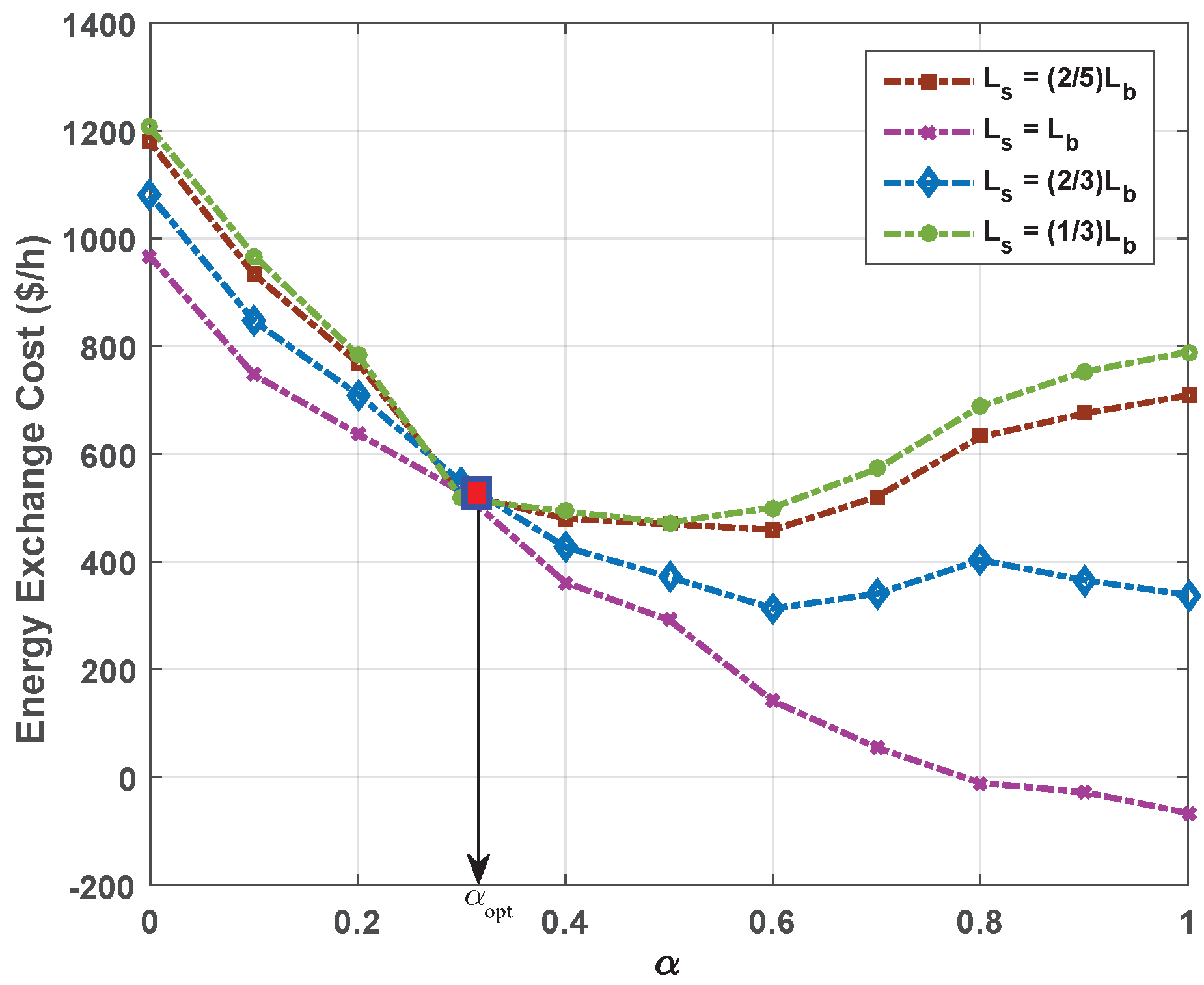
Table 6 shows the variation in due to different energy export prices. For any given value of and , increased with a decrease in . Note that optimal value of was different for each value of , even though these values were computed for the same location. In practice, it is not feasible to make changes to RES mix or the generation capacity once the whole system has been installed. Thus, one way to address this issue is by determining a compromise solution for that minimizes regardless of the variation in energy export costs. For this purpose, the variation in for all possible values of against is plotted in Figure 9. In this scenario, the optimized RES mix for Location C was given by the point of intersection of all the curves of .
5. Conclusions
This paper proposes the use of the complementary characteristic of RESs to achieve an economic and reliable operation of a microgrid. The proposed framework exploits the spatial and temporal solar-wind complementarity to maximize the economic benefits of a grid-tied microgrid. To locate regions where solar and wind exhibit substantial complementary behavior, meteorological data of different regions are gathered and complementarity value at each location is determined. Another significant aspect of maximizing the economic benefits is the RES mix that considerably affects the costs of energy production and energy exchange costs. Therefore, after identifying the complementarity value for a given location, the next step is to identify the optimized RES mix or the share of each RES, which is defined by the sharing coefficient. For this purpose, a constrained optimization problem is developed to minimize the energy exchange costs for all the possible RES mix values at a given location. It is shown that the cost of energy exchange for each sharing coefficient is dependent on the total system power loss, and there exists a minimum value of power loss for each RES mix, below which the energy exchange cost minimization problem becomes infeasible. However, at this minimum value of system power loss, the energy exchange cost may not be minimized. The optimal values of system power loss are found for each RES mix and determine the minimum energy exchange costs by solving the energy exchange cost minimization problem through particle swarm optimization.
The proposed model was verified through a case study on balanced IEEE 33-bus system. The results show that considerable reductions in energy exchange costs can be made by optimally selecting the threshold level of total system power loss and the sharing coefficient of RES mix. The framework thus allows the microgrid operator to decide on appropriate sharing coefficients to achieve various tradeoffs according to the energy production cost, solar-wind complementarity of the site and its required economic objectives.
Author Contributions
A.N. carried out the main research tasks and the manuscript preparation; N.U.H. supervised the entire work; and N.U.H., C.Y., and S.M.M. did the final editing and review of the manuscript.
Funding
This research was funded by Lahore University of Management Sciences (LUMS) FIF grant, SBASSE Dean pool, and Natural Science Foundation of China and Jiangsu Province (Project No. 61750110529, 61850410535, and BK20161147, respectively).
Conflicts of Interest
The authors declare no conflict of interest.
Appendix A. Computation of Solar-Wind Complementarity Value
Solar-wind complementarity value is determined by inserting values of the solar and wind energy potentials in Equation (6). This study considered four different locations, labeled , as shown in Figure 3. Due to different meteorological characteristics, a different solar-wind complementarity value for each of these locations was obtained. The variance and covariance are computed as follows,
Note that, in this study, average monthly values instead of daily or hourly mean values were used based on the assumption that the correlation between the monthly cumulative powers produced by these resources is a better indicator of seasonal influences. On the other hand, the hourly correlation is greatly affected by the day-night variations of sunlight, and the daily wind profile may not follow the same pattern on a similar day (e.g., see [32]).
Abbreviations
The following abbreviations are used in this manuscript:
| MG | Microgrid |
| RES | Renewable Energy Source |
| PV | Photovoltaic |
| ESS | Energy Storage System |
| SPL | System Power Loss |
| PSO | Particle Swarm Optimization |
| EPF | Exterior Penalty Function |
| LCOE | Levelized cost of electricity |
Nomenclature
| Indices/Sets | |
| N | Total number of nodes, indexed by i |
| M | Total number of renewable energy sources |
| T | Total time period, indexed by t |
| Parameters | |
| Conversion efficiency of solar PV panel | |
| A | Area of the PV panel |
| d | Discount factor |
| Y | Minimum of the life spans of solar and wind RES |
| Resistance of node i | |
| Cut-in speed at which the turbine starts generating power | |
| Rated power of wind turbine | |
| Rated speed of wind turbine | |
| Cut-off speed after which the turbine is shut down for safety purposes | |
| Maximum apparent power | |
| Variables | |
| Binary variable to indicate the presence of local RES at node i | |
| Active power generated by local RES at node i | |
| Reactive power generated by local RES at node i | |
| Active power generated at node i | |
| Reactive load demand at node i | |
| Active power loss occurring in section to i | |
| Reactive power loss occurring in section to i | |
| Active power transaction occurring with the power grid at time t | |
| Reactive power transaction occurring with the power grid at time t | |
| Active power produced by the solar PV units at node i, at time t | |
| Active power produced by the wind turbines at node i at time t | |
| Continuous variable ; represents the share of installed solar capacity at node i | |
| Step size of by which its value is varied | |
| Irradiance at node i at time t | |
| Wind speed at node i at time t | |
| Standard deviation of the energy produced by PV units at time t | |
| Standard deviation of the energy produced by wind turbines at time t | |
| Covariance of solar and wind energies at time t | |
| Solar-Wind complementarity value at a given location | |
| LCOE of RES mix, in | |
| Energy production cost of RES mix in a year | |
| Overall SPL | |
| Minimum value of SPL | |
| Optimal value of SPL | |
| Imported power component of at time t | |
| Exported power component of at time t | |
| Energy exchange cost at time t due to RES mix | |
| Annual Energy exchange cost due to RES mix at an optimal value of SPL | |
| Annual Energy exchange cost due to RES mix at any given value of SPL | |
| Net energy costs due to RES mix | |
| Investment cost of the RES mix at time t, where t is in years | |
| Operation and maintenance cost of RES mix at time t, where t is in years | |
| Fuel cost of RES mix (zero in case of solar and wind RES) at time t, where t is in years | |
| Energy produced by solar RES in a year | |
| Energy produced by wind RES in a year | |
| Average Energy produced by RES mix in a year | |
| Energy export price in $/kWh | |
| Energy import price in $/kWh | |
| SPL at time t | |
| Power loss in node i at time t | |
| Maximum power loss that ith bus can sustain | |
| Maximum power that can be imported from the grid | |
| Maximum amount of power that can be exported to the grid | |
| Penalties associated with violation of nth constraint at node i at time, t | |
| Apparent power at time t | |
| Reactive power of PV unit at node i at time t | |
| Reactive power of wind turbine at node i at time t | |
| Lower limit on reactive power from PV unit | |
| Upper limit on reactive power from PV unit | |
| Lower limit on reactive power from wind turbine | |
| Upper limit on reactive power from wind turbine | |
| Voltage at node i at time t | |
| Lower voltage limit at node i | |
| Upper voltage limit at node i | |
| Annual average value of either solar or wind RES; {solar, wind} | |
| Power potential of r at time instant, m where and {solar, wind} | |
| Variance of either solar or wind RES; {solar, wind} | |
| Covariance of solar and wind RES at time t |
References
- Zhang, C.; Xu, Y.; Dong, Z.Y.; Wong, K.P. Robust Coordination of Distributed Generation and Price-Based Demand Response in Microgrids. IEEE Trans. Smart Grid 2018, 9, 4236–4247. [Google Scholar] [CrossRef]
- Wang, Z.; Chen, B.; Wang, J.; Kim, J.; Begovic, M.M. Robust Optimization Based Optimal DG Placement in Microgrids. IEEE Trans. Smart Grid 2014, 5, 2173–2182. [Google Scholar] [CrossRef]
- Parhizi, S.; Khodaei, A.; Shahidehpour, M. Market-Based Versus Price-Based Microgrid Optimal Scheduling. IEEE Trans. Smart Grid 2018, 9, 615–623. [Google Scholar] [CrossRef]
- Bazrafshan, M.; Gatsis, N. Decentralized Stochastic Optimal Power Flow in Radial Networks With Distributed Generation. IEEE Trans. Smart Grid 2017, 8, 787–801. [Google Scholar] [CrossRef]
- Zachar, M.; Daoutidis, P. Microgrid/Macrogrid Energy Exchange: A Novel Market Structure and Stochastic Scheduling. IEEE Trans. Smart Grid 2017, 8, 178–189. [Google Scholar] [CrossRef]
- Georgilakis, P.S.; Hatziargyriou, N.D. Optimal Distributed Generation Placement in Power Distribution Networks: Models, Methods, and Future Research. IEEE Trans. Power Syst. 2013, 28, 3420–3428. [Google Scholar] [CrossRef]
- Tushar, W.; Zhang, J.A.; Yuen, C.; Smith, D.B.; Hassan, N.U. Management of Renewable Energy for a Shared Facility Controller in Smart Grid. IEEE Access 2016, 4, 4269–4281. [Google Scholar] [CrossRef]
- Chen, S.X.; Gooi, H.B.; Wang, M.Q. Sizing of Energy Storage for Microgrids. IEEE Trans. Smart Grid 2012, 3, 142–151. [Google Scholar] [CrossRef]
- Thirugnanam, K.; Kerk, S.K.; Yuen, C.; Liu, N.; Zhang, M. Energy Management for Renewable Microgrid in Reducing Diesel Generators Usage With Multiple Types of Battery. IEEE Trans. Ind. Electron. 2018, 65, 6772–6786. [Google Scholar] [CrossRef]
- Tushar, W.; Yuen, C.; Huang, S.; Smith, D.B.; Poor, H.V. Cost Minimization of Charging Stations With Photovoltaics: An Approach With EV Classification. IEEE Trans. Intell. Trans. Syst. 2016, 17, 156–169. [Google Scholar] [CrossRef]
- U.S. Energy Information Administration. U.S. Battery Storage Market Trends. 2018. Available online: https://www.eia.gov/analysis/studies/electricity/batterystorage/pdf/battery_storage.pdf (accessed on 17 December 2018).
- Huanna, N.; Lu, Y.; Jingxiang, Z.; Yuzhu, W.; Weizhou, W.; Fuchao, L. Flexible-regulation resources planning for distribution networks with a high penetration of renewable energy. IET Gener. Transm. Distrib. 2018, 12, 4099–4107. [Google Scholar] [CrossRef]
- He, G.; Chen, Q.; Kang, C.; Xia, Q.; Poolla, K. Cooperation of Wind Power and Battery Storage to Provide Frequency Regulation in Power Markets. IEEE Trans. Power Syst. 2017, 32, 3559–3568. [Google Scholar] [CrossRef]
- Kim, Y.; Kim, E.; Moon, S. Frequency and Voltage Control Strategy of Standalone Microgrids with High Penetration of Intermittent Renewable Generation Systems. IEEE Trans. Power Syst. 2016, 31, 718–728. [Google Scholar] [CrossRef]
- Risso, A.; Beluco, A.; Marques Alves, R.D.C. Complementarity Roses Evaluating Spatial Complementarity in Time between Energy Resources. Energies 2018, 11, 1918. [Google Scholar] [CrossRef]
- Zhang, X.; Ma, G.; Huang, W.; Chen, S.; Zhang, S. Short-Term Optimal Operation of a Wind-PV-Hydro Complementary Installation: Yalong River, Sichuan Province, China. Energies 2018, 11, 868. [Google Scholar] [CrossRef]
- Min, C.G.; Kim, M.K. Impact of the Complementarity between Variable Generation Resources and Load on the Flexibility of the Korean Power System. Energies 2017, 10, 1719. [Google Scholar] [CrossRef]
- Wang, H.; Huang, J. Joint Investment and Operation of Microgrid. IEEE Trans. Smart Grid 2017, 8, 833–845. [Google Scholar] [CrossRef]
- Bett, P.E.; Thornton, H.E. The climatological relationships between wind and solar energy supply in Britain. Renew. Energy 2016, 87, 96–110. [Google Scholar] [CrossRef]
- Atia, R.; Yamada, N. Sizing and Analysis of Renewable Energy and Battery Systems in Residential Microgrids. IEEE Trans. Smart Grid 2016, 7, 1204–1213. [Google Scholar] [CrossRef]
- Liu, Y.; Yuen, C.; Hassan, N.U.; Huang, S.; Yu, R.; Xie, S. Electricity Cost Minimization for a Microgrid With Distributed Energy Resource Under Different Information Availability. IEEE Trans. Ind. Electron. 2015, 62, 2571–2583. [Google Scholar] [CrossRef]
- Huang, W.T.; Yao, K.C.; Wu, C.C. Using the Direct Search Method for Optimal Dispatch of Distributed Generation in a Medium-Voltage Microgrid. Energies 2014, 7, 8355–8373. [Google Scholar] [CrossRef]
- Yousif, M.; Ai, Q.; Gao, Y.; Wattoo, W.A.; Jiang, Z.; Hao, R. Application of Particle Swarm Optimization to a Scheduling Strategy for Microgrids Coupled with Natural Gas Networks. Energies 2018, 11, 3499. [Google Scholar] [CrossRef]
- Yuan, R.; Li, T.; Deng, X.; Ye, J. Optimal Day-Ahead Scheduling of a Smart Distribution Grid Considering Reactive Power Capability of Distributed Generation. Energies 2016, 9, 311. [Google Scholar] [CrossRef]
- Farzin, H.; Fotuhi-Firuzabad, M.; Moeini-Aghtaie, M. A Stochastic Multi-Objective Framework for Optimal Scheduling of Energy Storage Systems in Microgrids. IEEE Trans. Smart Grid 2017, 8, 117–127. [Google Scholar] [CrossRef]
- Hou, H.; Xue, M.; Xu, Y.; Tang, J.; Zhu, G.; Liu, P.; Xu, T. Multiobjective Joint Economic Dispatching of a Microgrid with Multiple Distributed Generation. Energies 2018, 11, 3264. [Google Scholar] [CrossRef]
- Wei, C.; Fadlullah, Z.M.; Kato, N.; Stojmenovic, I. On Optimally Reducing Power Loss in Micro-grids with Power Storage Devices. IEEE J. Sel. Areas Commun. 2014, 32, 1361–1370. [Google Scholar] [CrossRef]
- Ahn, C.; Peng, H. Decentralized Voltage Control to Minimize Distribution Power Loss of Microgrids. IEEE Trans. Smart Grid 2013, 4, 1297–1304. [Google Scholar] [CrossRef]
- Naeem, A.; Hassan, N.U.; Yuen, C. Power Loss Minimization in Power Distribution Systems Using Wind and Solar Complementarity. In Proceedings of the 2018 IEEE Innovative Smart Grid Technologies—Asia (ISGT Asia), Singapore, 22–25 May 2018; pp. 1165–1170. [Google Scholar]
- Chughtai, A.H.; Hassan, N.U.; Yuen, C. Planning for Mitigation of Variability in Renewable Energy Resources using Temporal Complementarity. In Proceedings of the 2018 IEEE Innovative Smart Grid Technologies—Asia (ISGT Asia), Singapore, 22–25 May 2018; pp. 1147–1152. [Google Scholar]
- Miglietta, M.M.; Huld, T.; Monforti-Ferrario, F. Local Complementarity of Wind and Solar Energy Resources over Europe: An Assessment Study from a Meteorological Perspective. J. Appl. Meteorol. Clim. 2017, 56, 217–234. [Google Scholar] [CrossRef]
- Monforti, F.; Huld, T.; Bódis, K.; Vitali, L.; D’Isidoro, M.; Lacal-Arántegui, R. Assessing complementarity of wind and solar resources for energy production in Italy. A Monte Carlo approach. Renew. Energy 2014, 63, 576–586. [Google Scholar] [CrossRef]
- Halamay, D.A.; Brekken, T.K.A.; Simmons, A.; McArthur, S. Reserve Requirement Impacts of Large-Scale Integration of Wind, Solar, and Ocean Wave Power Generation. IEEE Trans. Sustain. Energy 2011, 2, 321–328. [Google Scholar] [CrossRef]
- Li, Y.; Agelidis, V.G.; Shrivastava, Y. Wind-solar resource complementarity and its combined correlation with electricity load demand. In Proceedings of the 2009 4th IEEE Conference on Industrial Electronics and Applications, Xi’an, China, 25–27 May 2009; pp. 3623–3628. [Google Scholar] [CrossRef]
- Khalid, M.; Savkin, A.V.; Agelidis, V.G. Optimization of a power system consisting of wind and solar power plants and battery energy storage for optimal matching of supply and demand. In Proceedings of the 2015 IEEE Conference on Control Applications (CCA), Sydney, Australia, 21–23 September 2015; pp. 739–743. [Google Scholar] [CrossRef]
- Romero, R.; Franco, J.F.; Leão, F.B.; Rider, M.J.; de Souza, E.S. A New Mathematical Model for the Restoration Problem in Balanced Radial Distribution Systems. IEEE Trans. Power Syst. 2016, 31, 1259–1268. [Google Scholar] [CrossRef]
- Tazvinga, H.; Zhu, B.; Xia, X. Energy dispatch strategy for a photovoltaic–wind–diesel–battery hybrid power system. Sol. Energy 2014, 108, 412–420. [Google Scholar] [CrossRef]
- Atwa, Y.M.; El-Saadany, E.F. Optimal Allocation of ESS in Distribution Systems With a High Penetration of Wind Energy. IEEE Trans. Power Syst. 2010, 25, 1815–1822. [Google Scholar] [CrossRef]
- Gholami, A.; Shekari, T.; Aminifar, F.; Shahidehpour, M. Microgrid Scheduling With Uncertainty: The Quest for Resilience. IEEE Trans. Smart Grid 2016, 7, 2849–2858. [Google Scholar] [CrossRef]
- EIA. Levelized Cost and Levelized Avoided Cost of New Generation Resources in the Annual Energy Outlook. 2018. Available online: https://www.eia.gov/outlooks/aeo/pdf/electricity_generation.pdf (accessed on 21 December 2018).
- Huang, Y.; Mao, S.; Nelms, R.M. Adaptive Electricity Scheduling in Microgrids. IEEE Trans. Smart Grid 2014, 5, 270–281. [Google Scholar] [CrossRef]
- Soroudi, A.; Siano, P.; Keane, A. Optimal DR and ESS Scheduling for Distribution Losses Payments Minimization Under Electricity Price Uncertainty. IEEE Trans. Smart Grid 2016, 7, 261–272. [Google Scholar] [CrossRef]
- Rao, R.S.; Ravindra, K.; Satish, K.; Narasimham, S.V.L. Power Loss Minimization in Distribution System Using Network Reconfiguration in the Presence of Distributed Generation. IEEE Trans. Power Syst. 2013, 28, 317–325. [Google Scholar] [CrossRef]
- El-Sayed, M.A.; Salama, M.M.; Farag, M.; Al-Thobaiti, F.B. The Cost Functional and Its Gradient in Optimal Boundary Control Problem for Parabolic Systems. Open J. Optim. 2017, 6, 26. [Google Scholar] [CrossRef]
- Khaled, U.; Eltamaly, A.M.; Beroual, A. Optimal Power Flow Using Particle Swarm Optimization of Renewable Hybrid Distributed Generation. Energies 2017, 10, 1013. [Google Scholar] [CrossRef]
- Srivastava, L.; Singh, H. Hybrid multi-swarm particle swarm optimisation based multi-objective reactive power dispatch. IET Gener. Trans. Distrib. 2015, 9, 727–739. [Google Scholar] [CrossRef]
- Garg, H. A Hybrid PSO-GA Algorithm for Constrained Optimization Problems. Appl. Math. Comput. 2016, 274, 292–305. [Google Scholar] [CrossRef]
- Baran, M.E.; Wu, F.F. Network reconfiguration in distribution systems for loss reduction and load balancing. IEEE Trans. Power Deliv. 1989, 4, 1401–1407. [Google Scholar] [CrossRef]
- Ellis, A.; Nelson, R.; Engeln, E.V.; Walling, R.; MacDowell, J.; Casey, L.; Seymour, E.; Peter, W.; Barker, C.; Kirby, B.; Williams, J.R. Reactive power performance requirements for wind and solar plants. In Proceedings of the 2012 IEEE Power and Energy Society General Meeting, San Diego, CA, USA, 22–26 July 2012; pp. 1–8. [Google Scholar]
- Ghosh, S.; Rahman, S.; Pipattanasomporn, M. Distribution Voltage Regulation Through Active Power Curtailment With PV Inverters and Solar Generation Forecasts. IEEE Trans. Sustain. Energy 2017, 8, 13–22. [Google Scholar] [CrossRef]
- Abugri, J.B.; Karam, M. Particle Swarm Optimization for the Minimization of Power Losses in Distribution Networks. In Proceedings of the 12th International Conference on Information Technology–New Generations, Las Vegas, NV, USA, 13–15 April 2015; pp. 73–78. [Google Scholar]
- Wang, C.; Cheng, H.Z. Optimization of Network Configuration in Large Distribution Systems Using Plant Growth Simulation Algorithm. IEEE Trans. Power Syst. 2008, 23, 119–126. [Google Scholar] [CrossRef]
- EIA. Electric Power Monthly. 2017. Available online: https://www.eia.gov/electricity/monthly/epm_table_grapher.php?t=epmt_5_3 (accessed on 23 October 2017).
- Editorial. Solar Power Buy-Back Rates. 2018. Available online: https://mysolarquotes.co.nz/about-solar-power/residential/solar-power-buy-back-rates-nz/ (accessed on 16 January 2019).
- Khodaei, A. Provisional Microgrid Planning. IEEE Trans. Smart Grid 2017, 8, 1096–1104. [Google Scholar] [CrossRef]
Figure 1.
Simplified MG Model under balanced conditions.
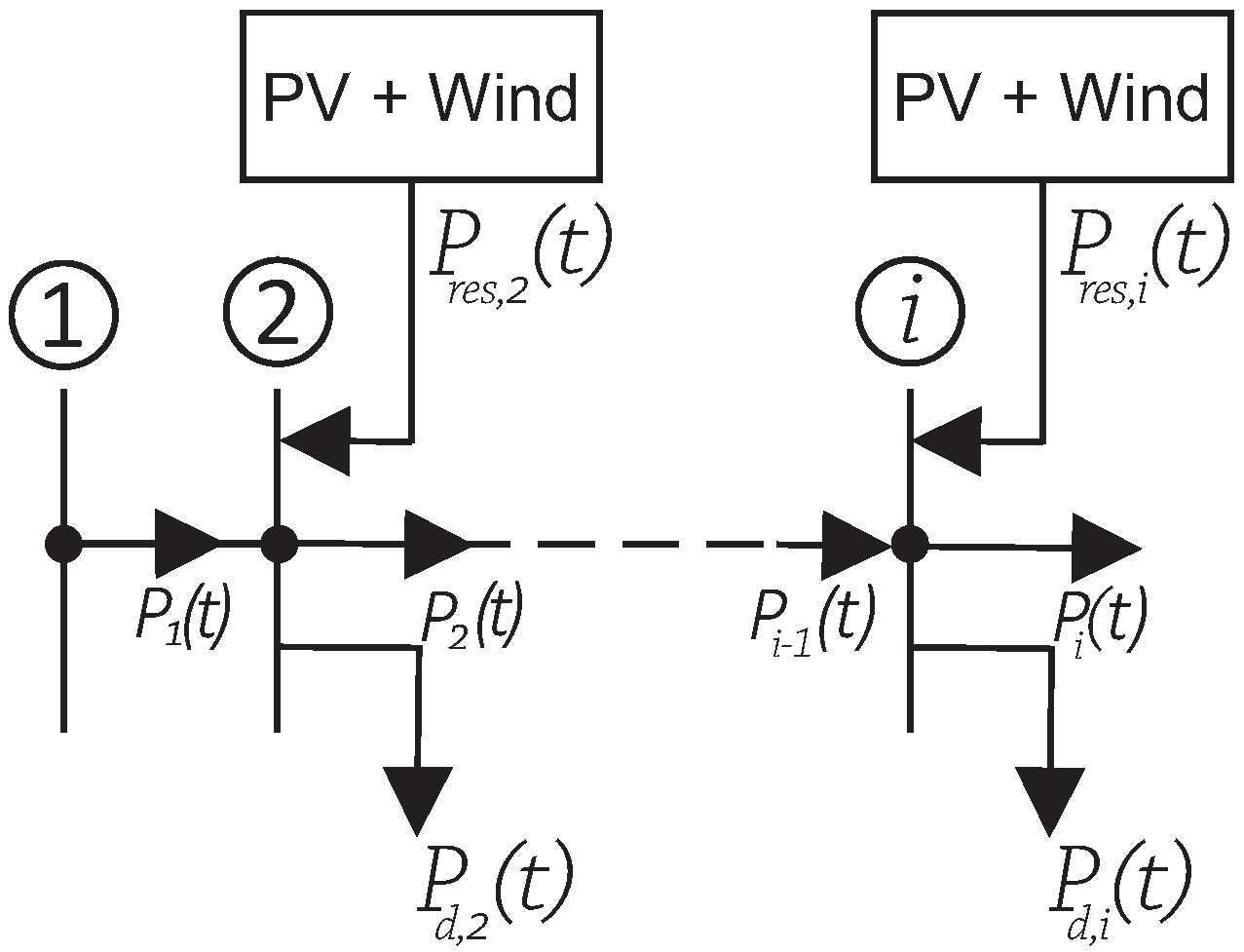
Figure 2.
Temporal Complementarity: Variations in mean monthly power production at a given location.
Figure 2.
Temporal Complementarity: Variations in mean monthly power production at a given location.

Figure 3.
Spatial Complementarity: Map of Ireland showing average complementarity values in different regions. Each of the four labeled sites has a different complementarity value.
Figure 3.
Spatial Complementarity: Map of Ireland showing average complementarity values in different regions. Each of the four labeled sites has a different complementarity value.
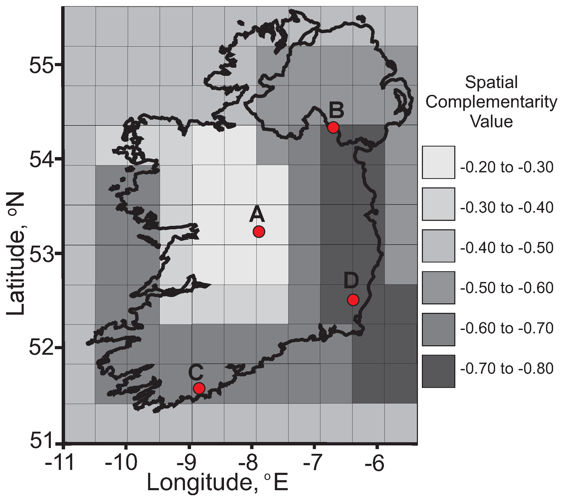
Figure 4.
Block diagram showing the proposed framework.
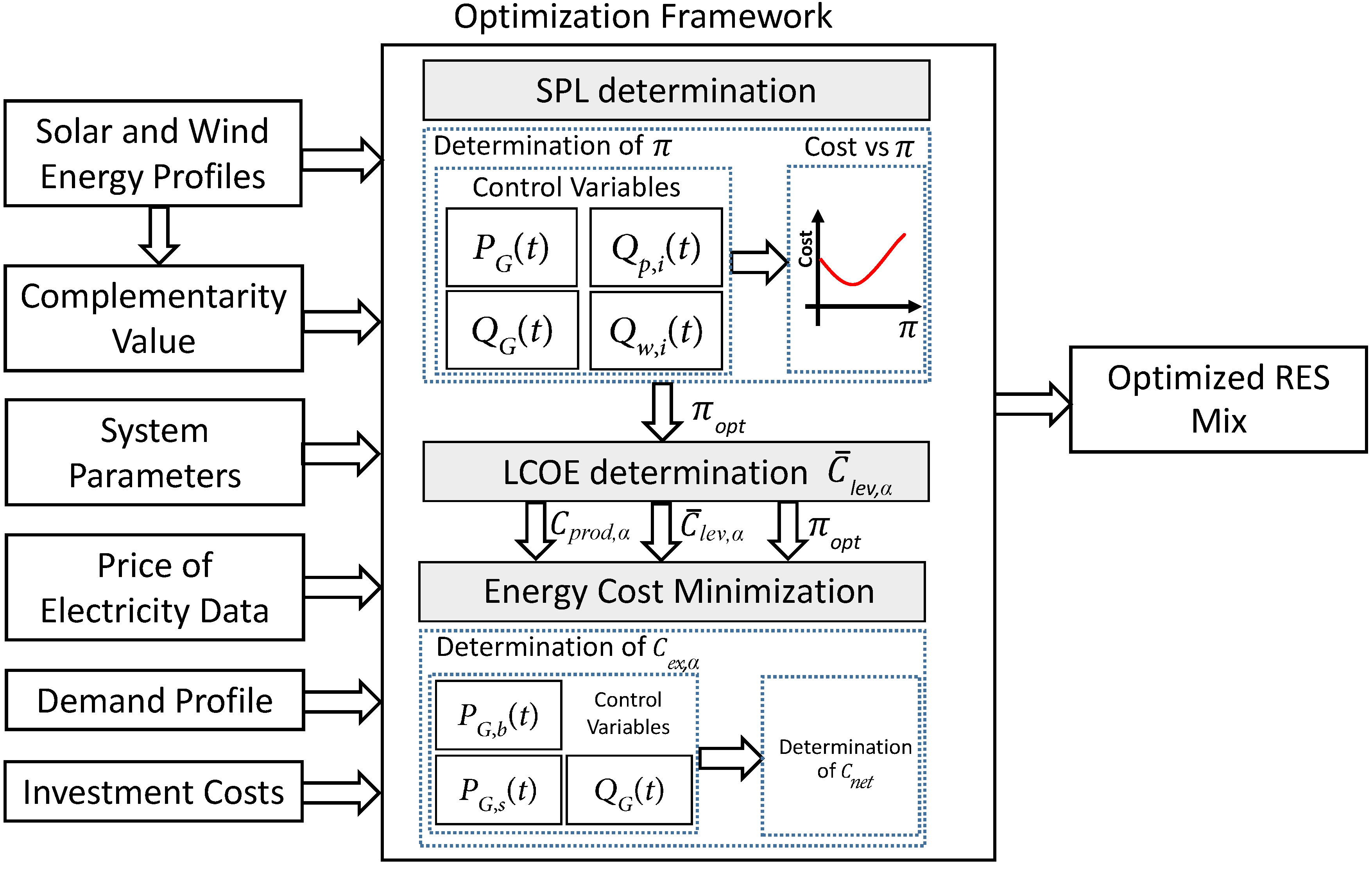
Figure 5.
Microgrid test system installed at each of the four selected locations.

Figure 6.
(a) Normalized surface solar radiation at Location C; and (b) normalized daily wind energy potential at Location C.
Figure 6.
(a) Normalized surface solar radiation at Location C; and (b) normalized daily wind energy potential at Location C.
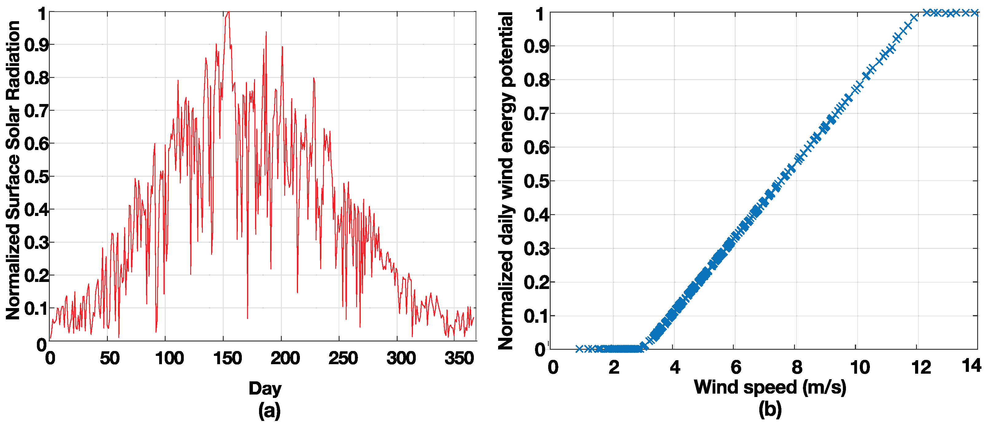
Figure 7.
Annual energy exchange cost, , against different threshold levels of total SPL, . Note that these results were plotted for Case-III with the average complementarity value of −0.66 with equal shares of RESs.
Figure 7.
Annual energy exchange cost, , against different threshold levels of total SPL, . Note that these results were plotted for Case-III with the average complementarity value of −0.66 with equal shares of RESs.

Figure 8.
Levelized cost of electricity, , for different values of .
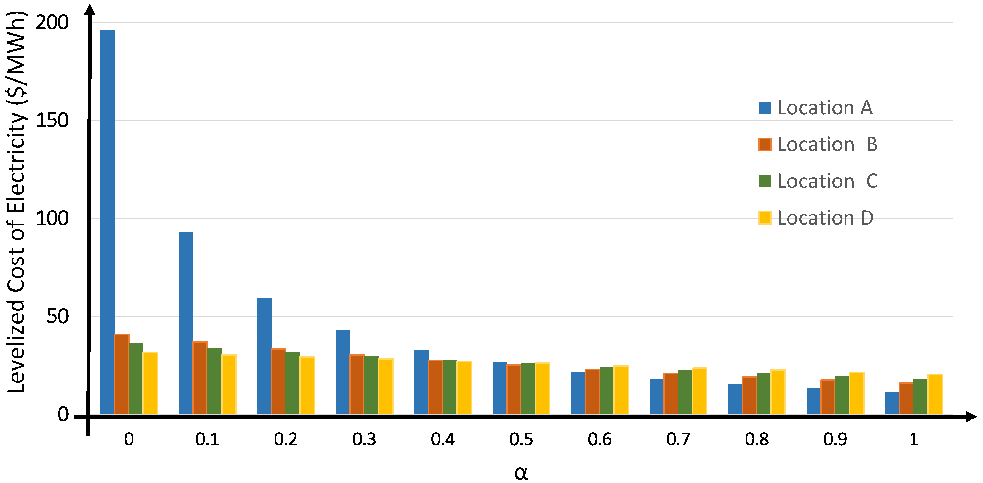
Figure 9.
Impact of different export prices on the annual energy exchange cost, . Note that these results have been plotted for Location C. The point of intersection gives .
Figure 9.
Impact of different export prices on the annual energy exchange cost, . Note that these results have been plotted for Location C. The point of intersection gives .

Table 1.
System configurations of grid-tied MG.
| Case Number | Sharing Coefficient, | Bus Index | Description |
|---|---|---|---|
| Case-I | 18, 32, 33 | PV only | |
| Case-II | 18, 32, 33 | Wind only | |
| Case-III | 18, 32, 33 | Both PV and Wind; share of solar RES is given by |
Table 2.
Solar-wind characteristics at different locations.
| Location | Complementarity Value, | Average Normalized Solar Irradiance | Average Normalized Wind Energy |
|---|---|---|---|
| A | −0.28 | 0.57 | 0.05 |
| B | −0.54 | 0.41 | 0.24 |
| C | −0.66 | 0.36 | 0.27 |
| D | −0.75 | 0.32 | 0.31 |
Table 3.
Influence of RES mix on the average annual SPL cost ($/h).
| Value of | Annual SPL Cost ($/h) at | |||
|---|---|---|---|---|
| A | B | C | D | |
| 1 | 146.5 | 93.8 | 75.3 | 73.3 |
| 0.9 | 139.8 | 85.7 | 70.4 | 66.4 |
| 0.8 | 87.5 | 74.4 | 64.1 | 59.8 |
| 0.7 | 76.5 | 61.5 | 46.1 | 49.8 |
| 0.6 | 54.1 | 59.1 | 42.2 | 51.4 |
| 0.5 | 46.9 | 44.7 | 31.3 | 41.4 |
| 0.4 | 32.5 | 38.1 | 28.7 | 39.0 |
| 0.3 | 26.8 | 36.4 | 32.8 | 39.9 |
| 0.2 | 20.6 | 39.7 | 32.6 | 43.4 |
| 0.1 | 20.5 | 35.8 | 27.5 | 48.8 |
| 0 | 30.3 | 33.2 | 33.1 | 56.7 |
Table 4.
Breakdown of the SPL cost ($/h) at Location C for different months of the year.
| Month | Case-I | Case-II | Case-III | Remarks |
|---|---|---|---|---|
| = 1 | = 0 | = 0.6 | ||
| Jan | 11.7 | 129.2 | 29.6 | Wind is more abundant; |
| Feb | 16.5 | 94 | 35.9 | Excess production in Case-II; |
| Mar | 33.5 | 23.9 | 32.1 | Solar irradiance levels are increasing; |
| Apr | 109.8 | 18.7 | 54.1 | excess production and SPL cost. |
| May | 181.2 | 12.8 | 94.6 | Combined local production exceeds |
| Jun | 181.2 | 11 | 63.5 | the demand; SPL cost rises |
| Jul | 151.2 | 14.9 | 78.3 | in Case-III during summer months |
| Aug | 109.8 | 16.6 | 42.9 | due to export of excess power |
| Sep | 54.5 | 30.1 | 29.9 | SPL cost in Case-III reduces |
| Oct | 16.6 | 11.5 | 21.8 | when combined local power production |
| Nov | 19.5 | 16.6 | 12.2 | matches the demand, leading to |
| Dec | 18.6 | 16.6 | 11.6 | minimum power exchange with grid |
| Average | SPL cost in Case-III reduced by 56% | |||
| Cost | 75.3 | 33 | 42.2 | relative to Case-I; but increased by |
| 27.8% relative to Case-II (solar excess) |
Table 5.
Effect of RES mix on the net costs, ($/h), for each location . The shaded values indicate the net costs for the optimal values of at each location.
Table 5.
Effect of RES mix on the net costs, ($/h), for each location . The shaded values indicate the net costs for the optimal values of at each location.
| Value of | Energy Production Cost, ($/h) | Energy Exchange Cost, ($/h) | Net Cost, ($/h) | |||||||||||
|---|---|---|---|---|---|---|---|---|---|---|---|---|---|---|
| A | B | C | D | A | B | C | D | A | B | C | D | |||
| 1 | 936.8 | 953.5 | 937.4 | 951.7 | −963.3 | 427.6 | 709 | 1118.6 | −26.5 | 1381.1 | 1646.4 | 2070.3 | ||
| 0.9 | 983.5 | 999.4 | 984.6 | 999.4 | −582.7 | 475.6 | 675.4 | 951.2 | 400.8 | 1475 | 1660 | 1950.6 | ||
| 0.8 | 1030.1 | 1044.9 | 1031.9 | 1047.2 | −416.6 | 476.3 | 632 | 822.9 | 613.5 | 1521.2 | 1663.9 | 1870.1 | ||
| 0.7 | 1066.8 | 1080 | 1069.3 | 1084.9 | −78.6 | 457.8 | 520.7 | 658.8 | 988.2 | 1537.8 | 1590 | 1743.7 | ||
| 0.6 | 1123.3 | 1134.7 | 1126.7 | 1142.7 | 261.4 | 569.1 | 459.4 | 571.5 | 1384.7 | 1703.8 | 1586.1 | 1714.2 | ||
| 0.5 | 1169.6 | 1178.8 | 1174.2 | 1190.5 | 593.3 | 531.6 | 470.1 | 375.2 | 1762.9 | 1710.4 | 1644.3 | 1565.7 | ||
| 0.4 | 1215.8 | 1222.4 | 1221.7 | 1238.3 | 1201.5 | 616.1 | 480.2 | 389.5 | 2417.3 | 1838.5 | 1701.9 | 1627.8 | ||
| 0.3 | 1261.6 | 1265.2 | 1269.4 | 1286.1 | 1855.9 | 854 | 525.4 | 413.4 | 3117.5 | 2119.2 | 1794.8 | 1699.5 | ||
| 0.2 | 1306.6 | 1307.2 | 1317.1 | 1333.9 | 2359.6 | 1200.2 | 769.2 | 522.9 | 3666.2 | 2507.4 | 2086.3 | 1856.8 | ||
| 0.1 | 1349.8 | 1348.1 | 1365 | 1381.7 | 3446.9 | 1457.5 | 933.8 | 678.8 | 4796.7 | 2805.6 | 2298.8 | 2060.5 | ||
| 0 | 1385.2 | 1387.9 | 1412.9 | 1429.6 | 4281.6 | 1757.9 | 1178.3 | 798.5 | 5666.8 | 3145.8 | 2591.2 | 2228.1 | ||
Table 6.
Influence of different energy export prices, on the energy exchange costs. Note that these values (in $/h) were obtained for Location C with a complementarity value of −0.66.
Table 6.
Influence of different energy export prices, on the energy exchange costs. Note that these values (in $/h) were obtained for Location C with a complementarity value of −0.66.
| Value of | ||||
|---|---|---|---|---|
| 1 | −66.4 | 338.4 | 709 | 789.5 |
| 0.9 | −27.7 | 365.8 | 675.4 | 753.0 |
| 0.8 | −10.6 | 403.3 | 632.0 | 688.6 |
| 0.7 | 55.0 | 340.7 | 520.7 | 572.5 |
| 0.6 | 141.3 | 313.4 | 459.4 | 500.8 |
| 0.5 | 291.7 | 371.8 | 470.1 | 473.1 |
| 0.4 | 361.4 | 427.2 | 480.2 | 493.3 |
| 0.3 | 529.8 | 547.3 | 525.4 | 517.1 |
| 0.2 | 637.6 | 710.5 | 769.2 | 783.8 |
| 0.1 | 747.3 | 846.7 | 933.8 | 968.2 |
| 0 | 966.2 | 1079 | 1178 | 1206 |
© 2019 by the authors. Licensee MDPI, Basel, Switzerland. This article is an open access article distributed under the terms and conditions of the Creative Commons Attribution (CC BY) license (http://creativecommons.org/licenses/by/4.0/).
Share and Cite
MDPI and ACS Style
Naeem, A.; Ul Hassan, N.; Yuen, C.; Muyeen, S.M. Maximizing the Economic Benefits of a Grid-Tied Microgrid Using Solar-Wind Complementarity. Energies 2019, 12, 395. https://doi.org/10.3390/en12030395
AMA Style
Naeem A, Ul Hassan N, Yuen C, Muyeen SM. Maximizing the Economic Benefits of a Grid-Tied Microgrid Using Solar-Wind Complementarity. Energies. 2019; 12(3):395. https://doi.org/10.3390/en12030395
Chicago/Turabian StyleNaeem, Aqsa, Naveed Ul Hassan, Chau Yuen, and S. M. Muyeen. 2019. "Maximizing the Economic Benefits of a Grid-Tied Microgrid Using Solar-Wind Complementarity" Energies 12, no. 3: 395. https://doi.org/10.3390/en12030395
Note that from the first issue of 2016, this journal uses article numbers instead of page numbers. See further details here.