Article

Development of a Space Heating Model Suitable for the Automated Model Generation of Existing Multifamily Buildings—A Case Study in Nordic Climate

1
School of Business, Society and Engineering, Mälardalen University, 72123 Västerås, Sweden
2
Eskilstuna Kommunfastighet AB, 63005 Eskilstuna, Sweden
3
Division of Building, Energy and Environment Technology, Department of Technology and Environment, University of Gävle, 80176 Gävle, Sweden
*
Author to whom correspondence should be addressed.
Energies 2019, 12(3), 485; https://doi.org/10.3390/en12030485
Submission received: 29 November 2018 / Revised: 22 January 2019 / Accepted: 30 January 2019 / Published: 2 February 2019
(This article belongs to the Special Issue Energy Performance and Indoor Climate Analysis in Buildings)

Abstract

:
Building energy performance modeling is essential for energy planning, management, and efficiency. This paper presents a space heating model suitable for auto-generating baseline models of existing multifamily buildings. Required data and parameter input are kept within such a level of detail that baseline models can be auto-generated from, and calibrated by, publicly accessible data sources. The proposed modeling framework consists of a thermal network, a typical hydronic radiator heating system, a simulation procedure, and data handling procedures. The thermal network is a lumped and simplified version of the ISO 52016-1:2017 standard. The data handling consists of procedures to acquire and make use of satellite-based solar radiation data, meteorological reanalysis data (air temperature, ground temperature, wind, albedo, and thermal radiation), and pre-processing procedures of boundary conditions to account for impact from shading objects, window blinds, wind- and stack-driven air leakage, and variable exterior surface heat transfer coefficients. The proposed model was compared with simulations conducted with the detailed building energy simulation software IDA ICE. The results show that the proposed model is able to accurately reproduce hourly energy use for space heating, indoor temperature, and operative temperature patterns obtained from the IDA ICE simulations. Thus, the proposed model can be expected to be able to model space heating, provided by hydronic heating systems, of existing buildings to a similar degree of confidence as established simulation software. Compared to IDA ICE, the developed model required one-thousandth of computation time for a full-year simulation of building model consisting of a single thermal zone. The fast computation time enables the use of the developed model for computation time sensitive applications, such as Monte-Carlo-based calibration methods.

Graphical Abstract

1. Introduction

Building energy performance modeling is essential for energy planning, management, and efficiency. To improve energy efficiency of building stocks, knowledge on how each building is currently performing is needed, often referred to as baselines. These baselines can for example be used to compare and rank building performance, estimate energy and cost saving potential of energy efficiency measures, and detect faults when systems are malfunctioning. Energy use of a building depends on aspects such as physical and thermal properties, climate, control and operational schemes, occupants’ presence, and behavior. Information regarding these aspects is often uncertain and scattered, sometimes missing altogether, and establishing the energy performance of buildings can therefore be a tedious task [1,2].
Building energy modeling is often categorized into two major approaches: law-driven (forward) and data-driven (inverse) [1,3]. Law-driven models apply a given set of physical laws that govern the system. Conversely, data-driven models use system behavior as a predictor for system performance. An advantage of data-driven models is that they generally require less input, while law-driven models can offer more flexibility regarding the fine adjustment of a building’s subsystems and components [1]. Examples of building energy simulation software that utilize a law-driven approach include EnergyPlus [4] and IDA ICE (https://www.equa.se/en/ida-ice). These types of software calculate building energy consumption based on detailed building and environmental information such as climate, operation schedules, building geometrics, and the shading/sheltering impact of the surroundings [1,2]. Examples of using law-driven simulation software for parameter identification can be found in Kang and Krarti [5], Tian et al. [6]. Data-driven modeling approaches have gained much research attention in recent years. The review article by Amasyali and El-Gohary [7] identified more than 50 articles using data-driven approaches. Weaknesses with data-driven approaches are that these may not perform well outside their training range and that statistical models yield limited knowledge of under-laying aspects that govern energy use. The main weaknesses of law-driven approaches are that they require detailed input and tend to model how the building is designed to operate and not how it actually operates.
Gray-box modeling combines law-driven and data-driven approaches, thereby leveraging the advantages and minimizing the disadvantages of both approaches, see for example Amasyali and El-Gohary [7], Bacher and Madsen [8], Boodi et al. [9]. In gray-box models, internal parameter and equations are physically interpretable and thus provide knowledge about the modeled building. Gray-box models are calibrated to better match a building’s actual operation performance, but can also provide physically reasonable results outside the training data range. The authors in Boodi et al. [9] recognized a need for more research efforts regarding model structures for gray box models for residential buildings.
The ISO 52016-1:2017 [10] standard, which replaces the older ISO 13790:2008 [11] standard, presents a set of calculation methods for a building energy needs and internal air temperatures. The hourly method described in the standard proposes a system of linear equations that model heat transfer through opaque and transparent components of the envelope and air exchange between the internal and external environments. The calculation result is hourly internal air and component temperatures and heating and cooling loads. Each construction component (e.g., roof, windows, and walls) is modeled as serially connected RC (resistance and capacitance) thermal networks. Compared to the old ISO 13790:2008 [11] standard, the new hourly method is a much closer representation of algorithms used in whole building simulation software, such as IDA ICE or EnergyPlus. The simplistic hourly method of the now deprecated ISO 13790:2008 [11] has been employed and explored in several scientific works, for example [12,13,14,15]. To the best of our knowledge, there has not yet been any scientific works employing the newer ISO 52016-1:2017 [10] standard.
Law-driven approaches require detailed input regarding the physical properties of the building. Most existing buildings were built before the era of modern BIM (building information modeling) and thus lack such information in digitized form. However, 3D shape representation of existing building can be achieved through the use of aerial images or LiDAR (light detection and ranging) or a combination of both [16]. Such 3D shape representations allow for the determination of buildings’ footprint, height, orientation, and surface areas. The Swedish Land Survey (Lantmäteriet) has collected LiDAR data for almost all of Sweden [17]. Parameters describing buildings’ thermal properties and technical system are, however, usually not readily accessible in a digitized format. Gray-box modeling approaches have proven successful for estimating such uncertain or unknown parameters [7,8,9].
Energy meter readings of high resolution are required for gray-box modeling approaches. In Sweden, since 2015, energy bills have been required to be based on actual energy consumption [18]. Therefore, most Swedish district heating system operators have automatic meter reading systems installed that gather hourly or sub-hourly readings to centralized databases. Most Swedish cities have extensive district heating networks, and district heating operators have an approximately 90% share of the heating market for multifamily buildings [19]. Approximately 94% of Swedish multifamily buildings have hydronic heating systems, and approximately 94% of these have thermostatic control valves installed [20].
From a Swedish multifamily building portfolio owner’s perspective (as energy strategist at Eskilstuna Kommunfastighet AB and corresponding author responsible for the energy performance of a 7000 apartment portfolio), it would be beneficial to have an energy performance model of each building—a model revealing both current and potential energy performance of the building. Such a model needs to be law-driven and detailed enough so that its parameters reveal meaningful and actionable information. However, the model also needs to be simple enough, so that basic models of existing buildings can be auto-generated from readily available data sources. It also needs to have a structure that allows calibration with actual meter readings, to ensure it represents the actual performance of the building and not only the intended/designed performance. A practical model fulfilling the above-mentioned requirements is currently missing: detailed simulation software (e.g., IDA ICE or EnergyPlus) requires too detailed input to be readily auto-generated and are too slow and complex to be readily calibrated, while the data-driven and gray-box models proposed in the literature are not detailed enough and too far from physics to reveal meaningful interpretable information. This paper presents a space heating model aiming at filling the identified gap.

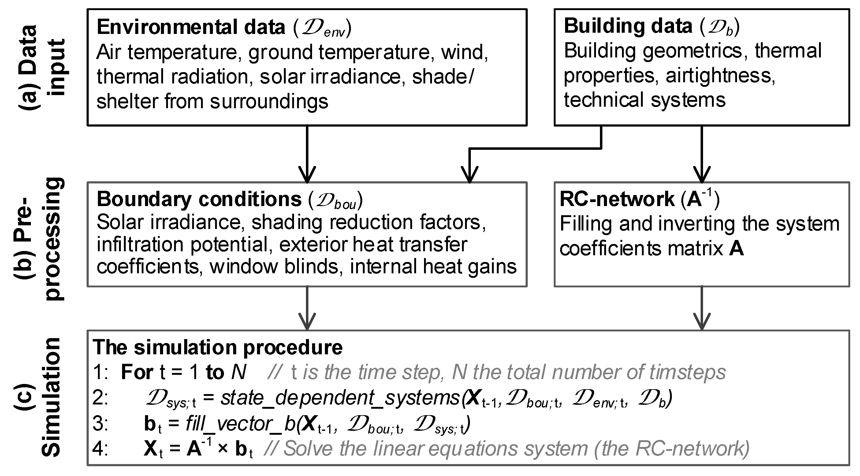
Methodology and Outline

The ISO 52016-1:2017 [10] standard employs an RC network to calculate hourly internal air temperatures, hourly heating and cooling loads, and space heating/cooling needs by summing the loads over certain time periods (e.g., monthly). This article presents the development of a thermal RC network that is based on the ISO 52016-1:2017 standard. However, our implementation is further simplified by lumping building elements by type and decreasing the number of temperature nodes in opaque building elements. Since the ISO 52016-1:2017 omits the conditions of use, the standard calculates the minimum energy need when assuming perfect temperature control and no system losses. To enable the calculation of actual energy use for space heating, comparable to metered values, a typical Swedish hydronic radiator heating system model [21,22] was implemented. Moreover, the following boundary condition procedures are proposed: a procedure to acquire satellite-based solar radiation data and conversion to a suitable format; a procedure to obtain and utilize meteorological reanalysis data (air temperature, ground temperature, wind, and thermal radiation and surroundings); procedures to account for impact from shading objects, window blinds, and wind- and stack-driven air infiltration, and variable exterior surface heat transfer coefficients. The developed model (including the RC network, heating system, and pre-processing steps) is from here on called ISO14N, where “ISO” denotes that it is based on the ISO 52016-1:2017 [10] standard and “14N” denotes the 14 temperature nodes (and 14 system equations). Figure 1 shows an overview of the proposed ISO14N modeling framework: from data input to pre-processing the boundary conditions data and constructing the RC network and to the simulation procedure.
As a validation, the simulation results were compared with results obtained with the well established and validated (https://www.equa.se/en/ida-ice/validation-certifications) simulation software IDA ICE. The main motivation behind using IDA ICE instead of the verification case provided by the ISO 52016-1:2017 [10] was that it also enabled testing the procedures that are not derived from the standard. Although the proposed RC network is generic, the use of a continuously operating hydronic radiator heating system and a constant air flow ventilation system limits the application of the proposed model to mainly multifamily buildings in Nordic climates. Therefore, the work is delimited to energy use for space heating for continuously heated multifamily buildings. Domestic hot water use, internal heat gains, and variable air flow ventilation are left for further work. Parallel work developing the calibration procedure, beyond the scope of this article, has been conducted and has influenced the design choices. The construction of the linear equation system of the RC network, the heating system, and the simulation procedure was implemented using the probabilistic programming language Stan [23], which parses to C++ code before compiling. The pre-processing procedures and the data input handling were implemented in the R statistical language based package dplyr [24]. Code can be requested from the corresponding author. The ISO 52010:2017 [25] standard (solar irradiance at an arbitrarily tilted and oriented surface) calculation procedure was implemented in C++ and published as an open source R-package (https://github.com/lukas-rokka/solarCalcISO52010).
The main features of the proposed ISO14N model are introduced in Section 2, while the pre-processing of the boundary conditions data is presented in Section 3. Section 4 describes the required data input and used data sources. Section 5.1, Section 5.2, Section 5.3, Section 5.4, Section 5.5, Section 5.6, Section 5.8, and Section 5.9 compare simulation results of the developed ISO14N model with results obtained with the IDA ICE. Section 5.7 show results from the proposed shading reduction. Details on constructing the linear equation system of the RC network are given in Appendix A.

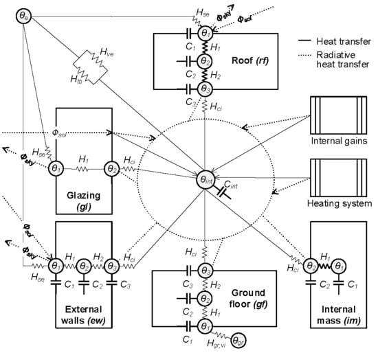
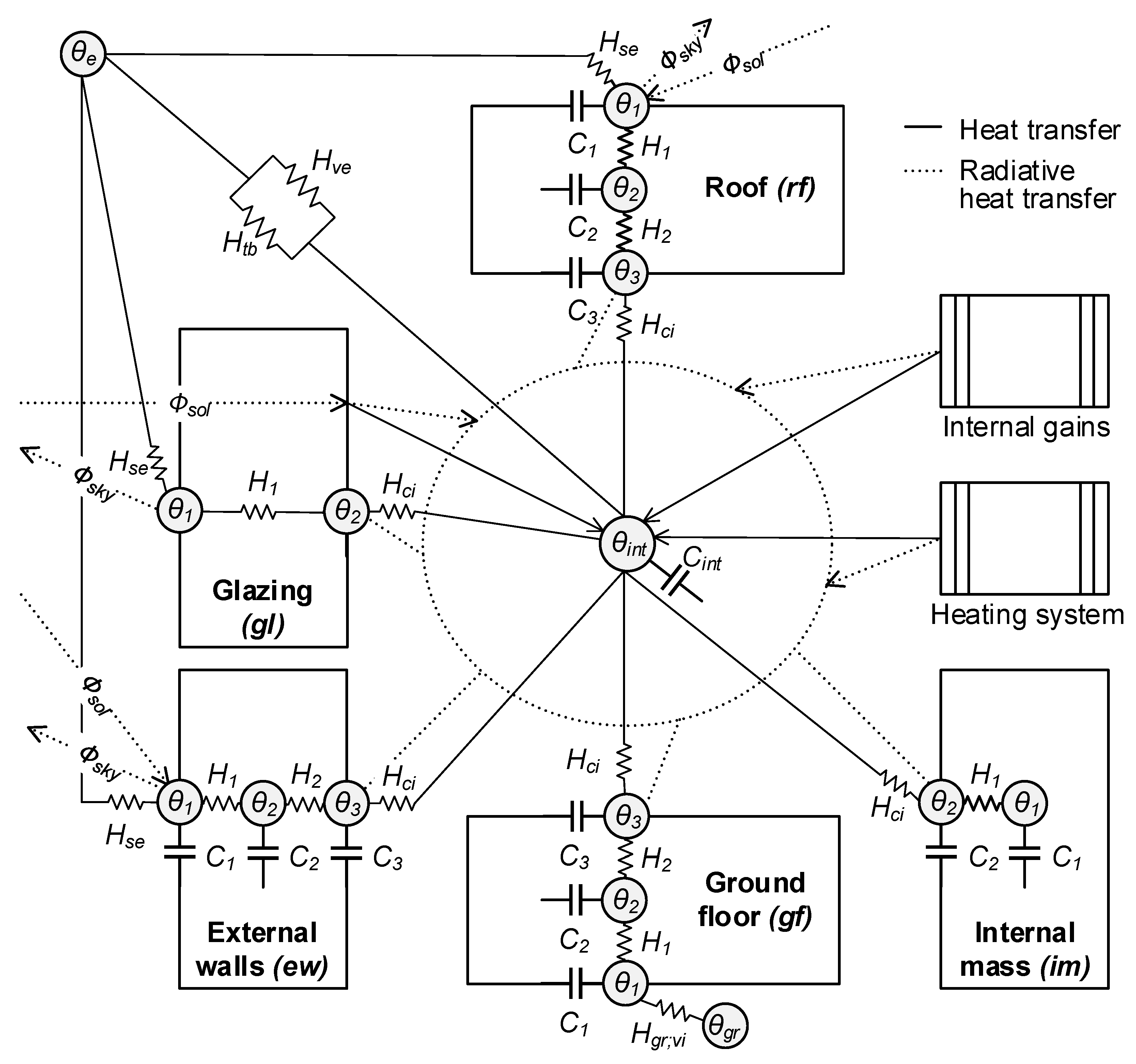
2. The ISO14N Space Heating Model

In this paper, a one-zone model representation for the whole building is illustrated. Figure 2 displays the proposed one-zone RC network. All external walls e w are modeled as a lumped 3-node element, all window glazing g l are modeled as a lumped 2-node element, and the external roof r f and the ground floor g f are modeled with 3-node elements. The remaining internal mass i m (internal walls, intermediate floors, and adiabatic external walls) are represented with a 2-node element. Thus, the thermal network consists of 14 unknown temperature nodes (including the internal air node θ i n t ). The thermal model can be represented as a system of linear equations:
A × X = b
where A is a 14 × 14 square matrix holding system coefficients, X is the state vector holding the 14 node temperatures, and b is a vector holding determined terms (node temperatures from the previous time step and known boundary condition values). Appendix A shows the details of the model matrices. For every time step t , the system of equations needs to be solved to compute the new states:
X t = A / b t = A 1 × b t .
Matrix inversion is computationally intensive. However, if matrix A only consists of constants, this computation step is only required once before the iterative simulation procedure. Vector b holds terms that can be treated as pre-processed data input (e.g., solar irradiance) and terms that need to be calculated at each simulation step due to dependence on the state of the node temperatures (e.g., thermal storage in nodes). Figure 1c shows the simulation procedure in pseudo code.

2.1. Geometrical and Thermal Properties

In this paper, the calculation is conducted normalized to per square meter floor (a deviation from the standard). One benefit is that geometrical data can be given as ratios (r) between the total interior surface area of each building element type and the total floor area (unit m s / m fl ). These ratios can be seen as weighting factors describing how large an impact one type of building element has on the average thermal balance of the whole building. It is straightforward to estimate these ratios from readily available building data:
r r f = r g f = 1 / N f l r e w = P · H f l · N f l / A f l r g l r i m = ( 2 2 / N f l ) + 1.5
where N f l is the number of floors of the building, A f l is the total floor area of the building, P is the building perimeter, and H f l is the average internal floor height. The term ( 2 2 / N f l ) in r i m calculates the surface area of internal floors and ceilings per total floor area and will result in a value between 0 and 2, depending on the number of floors. The additional 1.5 constant represents the internal walls, and it is based on the old ISO 13790:2008 [11] standard (where total interior surface area per total floor area is given as 4.5). The glazing-to-floor area ratio r g l is a property that is often regulated in standards and building codes, typically ranging between 0.1 and 0.2 for Swedish multi-family buildings.
Weighted surface heat transfer coefficients for each building element type are as follows: e l = [ r f , e w , g l , i m , g f ] , which are abbreviations of [roof, external walls, glazing, internal mass, ground floor]:
H s e ; r f ; t = r r f · ( h c e ; r f ; t + ( 1 F s k y ; h o r ) · 4.14 ) , H c i ; r f = r r f · 0.7 , H r i ; r f = r r f · 5.13 H s e ; e w ; t = r e w ( · h s e ; e w ; t + ( 1 F s k y ; v e r ) · 4.14 ) , H c i ; e w = r e w · 2.5 , H r i ; e w = r e w · 5.13 H s e ; g l ; t = r g l · ( h s e ; g l ; t + ( 1 F s k y ; v e r ) · 4.14 ) , H c i ; g l = r g l · 2.5 , H r i ; g l = r g l · 5.13 H c i ; i m = r i m · 2.5 , H r i ; i m = r i m · 5.13 H s e ; g f = r g f · h g r ; v i , H c i ; g f = r g f · 5.0 , H r i ; g f = r g f · 5.13
where H s e ; e l ; t [ W / ( K · m fl 2 ) ] represents normalized variable heat transfer coefficients (convective + radiative) between the exterior surface of the elements and external air at time step t, h c e ; e l ; t [ W / ( K · m s 2 ) ] represents exterior surface convective heat transfer coefficients at time step t (see Section 3.1), F s k y ; h o r and F s k y ; v e r are the sky view factors for horizontal and vertical elements respectively, h r e is the surface exterior radiative heat transfer coefficient, h g r ; v i is the heat transfer coefficient towards a virtual ground layer (see Equation (8)), H c i ; e l represents weighted convective heat transfer coefficients between the interior surface side of the elements and the internal air node, and H r i ; e l represents weighted radiative heat transfer coefficients of interior surface nodes. The constants are taken from ISO 52016-1:2017 [10] (Table 25) and describe conventional convective and radiative surface heat transfer coefficients for interior or exterior surfaces oriented upwards, horizontally, or downward.
In ISO 52016-1:2017 [10], opaque building elements (walls, roof, etc.) are by default described as 5-node and window glazing as 2-node elements. The distribution of the thermal resistances are slightly weighted towards the center of the building elements, while heat capacity nodes are weighted depending on chosen class (mass concentrated externally, internally, inside, or equally). In this paper, 3-node elements are used for opaque elements; therefore, there is less flexibility in distributing the thermal properties over the elements. The thermal resistance is equally distributed:
H 1 ; r f = H 2 ; r f = 2 / R r f , H 1 ; g l = 1 / R g l H 1 ; e w = H 2 ; e w = 2 / R e w , H 1 ; i m = 1 / R i m
where the floor area normalized thermal resistance R [ m fl 2 · C / W ] is calculated as
R e l = 1 / ( r e l · U e l ) 1 / ( H c i ; e l + H r i ; e l ) 1 / H s e ; e l
where U e l [ W / ( C · m s 2 ) ] is the thermal transmittance of building element e l . The heat capacity of 3-node building elements roof r f and external walls e w is distributed according to Table 1. The table is based on the ISO 52016-1:2017 [10] but altered to suit 3-node elements. Table B.14 of ISO 52016-1:2017 [10] specifies κ m values according to five classes (from very light to very heavy, 14–70 Wh / ( C · m s 2 ) ). The simulation procedure is conducted with normalized values, which are acquired by multiplying with surface ratios: C e l = r e l · κ m ; e l .
The internal mass i m building element is configured for 24 h thermal admittance cycles:
H 1 ; i m = 1 / 1.0 , κ 1 ; i m = 0.85 · κ m ; i m , κ 2 ; i m = 0.15 · κ m ; i m .
The ground floor element needs to account for effects of the ground, and its thermal resistance and heat capacity are distributed as follows:
H 2 ; g f = 2 / R g f , H 1 ; g f = 1 / ( R g f / 2 + R g r ) , H s e ; g f = r g r · h g r ; v i κ 3 ; g f = κ m ; g f / 2 , κ 2 ; g f = κ m ; g f / 2 , κ 1 ; g f = κ g r
where R g r and κ g r represent the thermal resistance and heat capacity of a 0.5 m thick soil layer (0.25 m s 2 · K / W and 280 Wh / ( K · m s 2 ) are used as default values), R g f is the thermal resistance of the ground floor including the effects of the ground, and h g r ; v i is the thermal transmittance of a virtual ground layer. R g f and h g r ; v i are calculated according to ISO 13370:2017 [26].

2.2. Hydronic Heating System

Heat dissipation from, in Sweden typically, a hydronic heating system with radiator panels, at time step t, can be approximated with the following non-linear equation [21,22]:
ϕ h y d ; t = H h y d · ( θ h y d ; l m t d ; t ) n h y d · u t r v ; t
where H h y d is the per floor square meter normalized radiator constant, n h y d is the radiator exponent (this depends on the design and type, but a value of 1.3 is commonly used for typical Swedish radiator panels [21,22]), u t r v ; t is the control signal from the local thermostatic radiator valve(s) (TRV), and θ h y d ; l m t d ; t is the logarithmic mean temperature difference between the radiator and the internal air temperature, which is calculated as
θ h y d ; l m t d ; t = θ h y d ; s u p ; t θ h y d ; r e t ; t ln θ h y d ; s u p ; t θ i n t ; t 1 ln θ h y d ; r e t ; t θ i n t ; t 1
where θ h y d ; s u p ; t and θ h y d ; r e t ; t are the supply/return temperatures to/from the radiators, θ i n t ; t 1 is the internal air temperature from the previous time step (internal air temperature is unknown at time step t until the linear equations system has been solved). The supply temperature θ h y d ; s u p is usually centrally controlled. For Swedish multifamily buildings, θ h y d ; s u p is usually controlled by linear interpolation from a look-up table. Such a look-up table consists of value pairs specifying supply temperature set-points θ h y d ; s u p ; s e t at certain external air temperature θ e . an example.
For a hydronic heating system without local TRVs, the following empirical equation was derived to estimate the return temperature:
θ h y d ; r e t ; t = θ h y d ; s u p ; t b · ( θ h y d ; s u p ; t θ i n t ; t 1 ) a a = n h y d Δ θ h y d ; d / 200 , b = Δ θ h y d ; d ( θ h y d ; s u p ; d θ i n t ; s e t ) a
where Δ θ h y d ; d is the temperature drop between supply and return temperatures at design power output, θ h y d ; s u p ; d is the supply temperature at design power output, and θ i n t ; s e t is the internal air set-point. Equation (11) was derived empirically and chosen to suit common Swedish radiator configurations. Validation is provided as Supplementary Materials. The TRV(s) are modeled as proportional controllers (P-controllers):
u t r v ; t = 0.5 · u t r v ; t 1 + 0.5 · max ( 0 , min ( 1 , ( θ i n t ; s e t θ i n t ; t 1 ) / θ t r v ; p b ) )
where θ i n t ; s e t is the set-point for desired indoor temperature, θ t r v ; p b is the proportional band of the TRV (typically ranging between 0.5–2.0 C ). Taking the average of current step and previous time step dampens oscillations in the control signal.

2.3. Ventilation

Heat transfer due to active ventilation is modeled as
ϕ v e ; t = κ ρ a · Q v e ; t · ( 1 η v e ) · ( θ i n t ; t 1 θ e ; t )
where κ ρ a is the heat capacity of air per volume 1.21 W · s / ( l · K ) , Q v e ; t is the specific air flow rate [ l / ( s · m fl 2 )], η v e is the temperature transfer efficiency of the heat recovery unit, θ i n t ; t 1 is the internal air temperature from the previous time step t, and θ e ; t is the external air temperature at current time step t.

2.4. Infiltration

Infiltration is driven by pressure differences across the building envelope caused by unbalanced mechanical ventilation, wind, and air temperature difference between internal and external air (known as the stack or buoyancy effect). One of the most established single zone models for estimating air infiltration rates is the Alberta air infiltration model (AIM-2), originally presented by Walker and Wilson [27] and referred to as the “enhanced model” in the ASHRAE Handbook—Fundamentals [3]. The AIM-2 model was developed for dwellings and has proven to be fairly accurate at estimating air infiltration rates for dwellings [28]. Hayati et al. [29] successfully used and evaluated the AIM-2 model for Swedish churches, modeled as large single zone models. The proposed thermal model of this paper is implemented as a single zone model, but this single zone is a representation of the average of a whole building (that could be a height of several floors). Thus, the AIM-2 model is implemented with modifications as to make the model more suitable for multi-floor buildings. Compared to earlier representations [3,27,28,29], equations are presented such that parameters are separated from parts that can be treated as pre-calculable data input. Thermal power losses due to infiltration are calculated as
ϕ i n f ; t = C i n f · Q i n f ; t * · κ ρ a · ( θ i n t ; t 1 θ e ; t )
where C i n f [ l / ( s · Pa n · m fl 2 ) ] is the infiltration coefficient (often referred to as the flow coefficient), n is the flow exponent, κ ρ a is the heat capacity of air per volume [1.21 Ws / ( l · C ) ], and Q i n f * is the potential specific air flow rate [ Pa n ] due to air infiltration. Q i n f * is pre-calculated (see Section 3.2), the flow exponent n is treated as a constant ( n = 0.73 [30]), while C i n f needs to be provided as an input parameter.

2.5. Radiant Heat Gains Exterior Surfaces

Net radiant heat gains on exterior surfaces due to thermal radiation exchange with the sky dome and absorption of solar irradiance are expressed as
ϕ r e ; r f ; t = r r f · ( α s o l · I t o t ; h o r ; s h ; t ϕ s k y ; r f ; t ) ϕ r e ; e w ; t = r e w · ( α s o l · I t o t ; v e r ; s h ; t ϕ s k y ; e w ; t ) ϕ r e ; g l ; t = r g l · ( ϕ s k y ; g l ; t )
where r is the weighting ratio of the element, α s o l is the solar absorption coefficient of the exterior surface (0.5 is used as default), I t o t is the calculated total hemispherical solar irradiance (see Section 3.3), ϕ s k y is the extra thermal radiation to the sky, subscript v e r denotes vertical surfaces, subscript h o r denotes horizontal surfaces, and subscript s h denotes shading. Thermal radiation exchange with the surrounding environment is accounted for in Section 3.1. The extra thermal radiation to the sky variable follows the definition used in [10] (positive values denote heat loss; negative values denote heat gains). However, an alternative calculation procedure is proposed so that it can be derived from climate model data sources:
ϕ s k y ; e l ; t = F s k y ; e l · ϵ e l · ( σ · ( θ 1 ; e l ; t 1 + 273.15 ) 4 ϕ s t r d )
where F s k y ; e l is the sky view factor for element e l (0.5 used for vertical elements external walls and glazing and 1.0 used for the horizontal roof element), ϵ is the emissivity of the surfaces (0.9 used as default), θ 1 ; e l is the exterior surface temperature of the element e l , σ is the Stefan–Boltzmann constant (5.67 × 10 8 W / ( m 2 · K 4 ) ), 273.15 is the Kelvin to Celsius conversion constant, and ϕ s t r d is the “surface thermal radiation downwards” variable retrieved from the climate reanalysis dataset ERA5 (see Section 4.2).

2.6. Radiant Heat Gains Interior Surfaces

Interior surfaces are subjected to solar and thermal radiation, expressed as
ϕ r i ; e l ; t = f e l · ( f r ; s o l · ϕ s o l ; g l ; t + f r ; i n t · ϕ i n t ; t + f r ; h y d · ϕ h y d ; t )
where f e l is the surface area fraction of the element e l , and f r is the fraction of radiative heat ( f r = 1 f c ). Default convective fractions from the ISO 52016-1:2017 [10] standard: f c ; s o l = 0.1 , f c ; i n t = 0.4 , and f c ; h y d = 0.4 . The surface area fractions f e l are simply calculated by dividing the ratio (r) of each building element with the sum of all ratios of the five building element types.

2.7. Operative Temperature

The ISO 52016-1:2017 [10] calculates operative temperature as follows:
θ o p ; t = 0.5 · ( θ i n t ; t + θ i n t ; r ; m n ; t )
where θ i n t ; r ; m n is the mean radiant temperature, calculated as the area weighted mean of interior surface temperatures of all building elements. However, Equation (18) omits the impact of radiative heating from the hydronic heating system. With radiator panels of the known surface area and surface temperatures, their contribution to the operative temperature can be area-weighted in the same manner as interior walls. An equation that does not require such detailed knowledge of the heating system is proposed:
θ o p ; t = 0.5 · ( θ i n t ; t + θ i n t ; r ; m n ; t + C h y d ; r ; m n · f r ; h y d · ϕ h y d ; t )
where C h y d ; r ; m n is a weighting and conversion coefficient expressing the impact of the radiative heating part of the hydronic heating system on the operative temperature. The unit of the C h y d ; r ; m n parameter is the same as that of a floor area normalized thermal resistance, m fl 2 · C / W .

3. Pre-Processing of Boundary Conditions Data

3.1. Convective Heat Transfer Coefficients for Weather-Exposed Exterior Surfaces

The ISO 52016-1:2017 [10] standard provides constant conventional surface heat transfer coefficients for exterior surfaces ( h c e ). However, h c e varies strongly depending on weather conditions [31,32]. Here, we implement the correlation equations by Liu et al. [32], derived by computational fluid dynamic calculations. Compared to earlier works [31], Liu et al. [32] accounts for wind sheltering effects, and separate correlations factors are provided for vertical walls and the roof. Additionally, our implementation accounts for surface roughness by adopting parts of the DOE-2 convection model [4] method.
h c e ; r f ; t = h c ; n + R f ; r f · h c ; n 2 + h c ; f ; h o r ; t 2 h c ; n h c e ; e w ; t = h c ; n + R f ; e w · h c ; n 2 + h c ; f ; v e r ; t 2 h c ; n h c e ; g l ; t = h c ; n 2 + h c ; f ; v e r ; t 2
where h c ; n is the natural convective heat transfer coefficient, h c ; f is the forced (wind effects) convective heat transfer coefficient, and R f is the surface roughness multiplier. The surface roughness multiplier is set as smooth R f ; r f = 1.11 for the roof and as medium rough R f ; e w = 1.52 for external walls [4]. The authors in Liu et al. [32] calculated the natural convective heat transfer coefficient as depending on temperature difference between external air and the exterior surface of the building element: h c ; n ; t = 1.52 · Δ θ t 0.36 W / ( K · m s 2 ) . Here we assume a constant temperature difference of Δ θ = 5 C , which results in a constant h c ; n = 2.7 W / ( K · m s 2 ) . Assuming h c ; n as a constant allows treating Equation (20) as pre-calculable data input. Wind has the strongest impact on the exterior surface convective heat transfer, and the forced heat transfer coefficients are calculated as
h c ; f ; v e r ; t = F w w · ( 3.39 5.03 · λ p ) · U l o c ; v e r 0.94 + ( 1 F w w ) · ( 1.15 + 0.82 · λ p ) · U l o c ; v e r 0.94 h c ; f ; h o r ; t = ( 3.57 + 1.72 · λ p ) · U l o c ; h o r 0.84
where F w w is the fraction of windward-oriented exterior surfaces, λ p is the plan area density, and U l o c is the local wind speed. F w w is assumed as a constant of 0.5 but could also be calculated as a variable depending on wind orientation using an approach similar to that taken for solar irradiance in Equation (29). The plan area density λ p represents the projected built area viewed from above to the total area in consideration [32]. Conceptually it relates to the wind sheltering factor used for the wind infiltration calculation (see Equation (26)), and here we present them in the same table, Table 2, and categorize the λ p values used in [32] into the sheltering classes defined in Table 5, Chapter 16 ASHRAE [3]. The local wind speeds are calculated according to Equation (22), where the height H is set as the building height for horizontal surfaces and half the building height for vertical surfaces.
U l o c = U 10 m · 1.59 · H l o c δ α
where U 10 m is the meteorological wind speed at 10 m height, the constant 1.59 describes the terrain conditions of the meteorological wind speed measurement site, H l o c is the height above ground for local wind calculation point, and δ and α are atmospheric boundary layer coefficients for different terrain categories, provided, e.g., in Table 1 of Chapter 24 of the ASHRAE Handbook—Fundamentals [3] ( δ = 370 and α = 0.22 for urban and suburban terrain).

3.2. Infiltration Potential

Potential air infiltration from wind-driven and stack-effect-driven infiltration is not additive, which in the AIM-2 [3] is modeled with the following superposition formula:
Q i n f ; t * = ( Q s ; t * ) 1 n + ( Q w ; t * ) 1 n 0.33 · ( Q s ; t * · Q w ; t * ) 1 2 n n
where the flow exponent n is treated as a constant ( n = 0.73 [30]), and Q s * and Q w * are the contributions of the stack and the wind effects. Compared to the original formula [3,27], Equation (23) is modified such that Q * = Q / C i n f [ Pa n ]. The contribution due to stack effect is calculated as
Q s ; t * = C s · ρ a · g 0 · H * · | θ i n t ; s e t θ e ; t | θ i n t ; s e t + 273.15 n
where C s [ ( Pa / K ) n ] is the stack coefficient, ρ a [ kg / m 3 ] is the density of air, g 0 [ m / s 2 ] is the acceleration of gravity, H * [ m ] is the modified building’s ceiling height, θ i n t ; s e t is the internal temperature set point, and θ e ; t is the external air temperature at time step t. The set point temperature is used instead of the actual internal air temperature so that Equation (24) can be treated as a pre-calculable data variable. The AIM-2 model was originally designed as a single zone model for residential building with up to three floor levels, assuming free air contact between the floor levels. Using the model as such for high rise buildings would probably overestimate the stack effect. Thus, a modified building height parameter H * is introduced:
H * = N f l · 0.5 · H f l if N f l < 3 N f l · 0.5 · H f l / 3 if N f l 3
where N f l is the number of floor levels, and 0.5 · H f l is half the average floor height. The rationale behind dividing by 3 for non-dwelling buildings with three or more floor levels is that the stack effect of such buildings will be a mix of the per zone/floor level height-induced stack effect and the whole building stack stack effect due to elevator shafts and stairways. The contribution due to wind effect is calculated as
Q w ; t * = C w · ρ a · λ w · U l o c 2 2 n
where the C w [ ( Pa · s 2 / m 2 ) n ] is the wind coefficient, λ w is the wind sheltering factor given in Table 2, and U l o c is the local wind speed at the building’s uppermost eaves height calculated with Equation (22).
In the AIM-2 air infiltration model [27], the stack and wind coefficients ( C s and C w ) can be calculated as functions of leakage distribution, occurrence of flue, and the type of foundation (crawlspace, basement, or slab-on-grade) [27]. Assuming evenly distributed leakage, no flue, and slab-on-grade foundation, C s = 0.25 [ ( Pa / K ) n ] and C w = 0.22 [ ( Pa · s 2 / m 2 ) n ] . The infiltration coefficient C i n f is given in liters instead of cubic meters and normalized to square meter floor. Otherwise, it is the same coefficient as described in [3,27]. Thus, it can be derived from building air leakage databases or from measurements (such as blower door pressurization tests).

3.3. Solar Heat Gains

Solar heat gains transmitted through windows glazing ( g l ) are calculated as
ϕ s o l ; g l ; t = r g l · g g l · g b l · I t o t ; v e r ; s h ; t
where I t o t ; v e r ; s h ; t [ W / m s 2 ] is the (by surface orientation) weighted hemispherical solar irradiance on vertical surfaces including shading effects, g b l is the total solar energy transmittance of the window blinds (see Section 3.5), g g l is the total solar energy transmittance of the glazing, and r g l is the glazing-to-floor ratio. I t o t ; v e r ; s h ; t is calculated as
I t o t ; v e r ; s h ; t = I d i f ; v e r ; t + I d i r ; v e r ; t · F s h ; v e r ; t
where I d i f ; v e r ; t and I d i r ; v e r ; t are the total diffuse (inclusive ground reflectance and exclusive circum-solar) and the total direct (inclusive circum-solar) irradiance received on one square meter of weighted vertical surface area at time step t, and F s h ; v e r ; t is a shading factor (see Section 3.4). Building elements are lumped according to their type, so solar irradiance variables also need to be allocated and weighted accordingly:
I d i f ; v e r ; t = k = 1 n γ F γ k · I d i f ; v e r ; γ k ; t I d i r ; v e r ; t = k = 1 n γ F γ k · I d i r ; v e r ; γ k ; t
where I d i r ; v e r ; γ k ; t is the total direct solar irradiance at a vertical surface with azimuth γ and time step t, F γ k is the surface area fraction of external walls at azimuth γ k , and n γ is the total number of surfaces of different azimuths to loop through. The same procedure is used for I d i f ; v e r ; t . For example, solar irradiance for the cardinally oriented cube would be calculated using F γ = [ 0.25 , 0.25 , 0.25 , 0.25 ] and γ = [ 0 , 90 , 90 , 180 ] .
The solar irradiance absorbed by the roof needs its own variable. The calculation procedure is the same as that for the vertical surfaces. However, there is no need for area weighting as the roof is assumed to be representable with one horizontal surface:
I t o t ; h o r ; s h ; t = I d i f ; h o r ; t + I d i r ; h o r ; t · F s h ; h o r ; t .
The solar irradiance at an arbitrarily tilted and oriented surface is calculated accordingly to the ISO 52010:2017 [25] standard. The calculation procedure was implemented in C++/R and validated against the accompanying test data of the the standard. The code with validation/unit tests is published under a public domain license and is located at the first author’s GitHub code repository (https://github.com/lukas-rokka/solarCalcISO52010).

3.4. Shading Reduction Factor

Distant obstacles (hills, trees, buildings etc) and obstacles on or nearby the building (balconies, rebates etc.) block parts of the solar radiation reaching a buildings surface. For best accuracy, these are calculated according to the actual surroundings of the building site. However, one of the goals with this work was to make reasonable estimates without actual information of the surroundings. Therefore, the shading factors are calculated based on assumptions about what the surroundings of a typical Swedish urban multifamily building typically look like. The resulting estimation can be expected to be more accurate on average than if shading were not accounted for at all. The shading reducing factor for the vertical envelope is calculated as
F s h ; v e r ; t = ( α s o l ; t > 0 ) · ( F s h ; o b s t ; t + F s h ; o v h ; t 1 )
where F s h ; o b s t is the shading from obstacles, and F s h ; o v h is the shading from overhangs on the buildings. The shading factor for infinite length overhangs is calculated as described by Method 2 in Annex F of ISO 52016-1:2017 [10]:
F s h ; o v h ; t = 1 max ( 0 , min ( 1 , ( D o v h · tan ( α s o l ; t ) L o v h ) / H g l ) )
where D o v h is the depth of the overhang, α s o l is the solar altitude, L o v h is the vertical distance between the glazing and the overhang, and H g l is the height of the window glazing. Many buildings have balconies; to account for this to at least some extent, the following values were used D o v h = 2 m , L o v h = 1 m , and H g l = 6 m . Setting H g l = 6 m is approximately the same as having overhangs above every 4th window of a more typical window glazing height of 1.5 m .
The shading reduction factor calculation for distant obstacles is calculated as a mix of two semitransparent obstacles:
F s h ; o b s t ; t = 1 min ( H b , max ( 0 , H o b s t ; 1 λ s o l · L o b s t ; 1 · tan ( α s o l ; t ) ) ) / H b + min ( H b , max ( 0 , H o b s t ; 2 λ s o l · L o b s t ; 2 · tan ( α s o l ; t ) ) ) / H b
where L o b s t is the distance between the shading obstacle and the shaded object, H o b s t is the height of the obstacle, H b is the height of the shaded building, and λ s o l is a shading factor set based on the categorization of the surroundings of the building (see Table 2). Obstacle 1 models nearby objects such as trees, and its parameters are set as L o b s t ; 1 = 15 m and H o b s t ; 1 = 20 m . Obstacle 2 models shading from other buildings, and its parameters are set as a function of the building height L o b s t ; 2 = H b and H o b s t ; 2 = 1.3 · H b . Shading at the roof level is calculated as
F s h ; h o r ; t = min ( 3 , H b H o b s t ; 1 ) / 3 · 0.5 + 0.5 .

3.5. Window Blinds

Window blinds exist in most Swedish residential buildings. However, there is no comprehensive consensus about the way people operate blinds or the motivating factors that influence their decisions [33]. A Swedish survey by Sandberg and Engvall [34] showed a clear correlation between exposure to solar radiation and to both the occurrence and position of window blinds. The g-value of the window blinds at time interval t is calculated as
g b l ; t = 1 + ( g b l ; m a x 1 ) · u b l ; t
where g b l ; m a x is a parameter describing the g-value of the blinds when at maximum blocking capacity, and u b l ; t is the control signal to the blinds. If the window blinds were automatically operated, the u b l ; t could for example be modeled as an on/off signal depending on solar radiation and a threshold value. The following function attempts to deterministically estimate the control signal of occupant operated window blinds:
u b l ; t = max ( 0.3 , min ( 0.7 , I t o t ; w m a ; t / 200 ) ) I t o t ; w m a ; t = k = 0 h 23 h 24 k 300 · I t o t ; t k
where the max and min functions limit the control signal between 30 and 70%, and I t o t ; w m a ; t is a weighted moving average of solar radiation exposure from the last 24 h. The motivation behind using weighted moving average was to model the position of the blinds as depending both on the current (active control) and recent (reactive control) solar radiation exposure. The use of a 24 h moving average will also result in a seasonal effect, as there are more hours with no solar radiation in winter than in the summer (modeling occupants as slightly more aware of the positions of the blinds in the summer season seems to be based on a reasonable assumption). The motivation behind limiting the control signal between the somewhat arbitrary 30 and 70% was that it can be expected that some blinds are also drawn in a situation of no solar exposure, that it is unlikely that all windows have blinds, and/or that these are in full position in a situation of high solar exposure.

4. Data Input

Section 4.1 and Section 4.2 describe the environmental data sources proposed for the ISO14N modeling framework. For the comparison study, environmental data for Norrköping, Sweden ( 58.575 N, 16.15 E) and the year 2016 was used. Section 4.3 describes the example model building as implemented in IDA ICE and ISO14N.

4.1. Solar Irradiance

Direct normal and diffuse horizontal irradiance data were acquired from CAMS [35] (http://www.soda-pro.com/web-services/radiation/cams-radiation-service). This satellite-based solar irradiance data are available at a horizontal resolution of 5 km and 15 min time steps from 2004 until the present time, and covers Europe, Africa, and the Middle East.

4.2. Meteorological Reanalysis Data

Table 3 shows which variables were acquired from the reanalysis climate dataset ERA5 of the Copernicus Climate Change Service. ERA5 data are available at a global horizontal resolution of 31 km and hourly time steps [36] (https://cds.climate.copernicus.eu/cdsapp). Reanalysis uses numerical weather prediction schemes to assimilate historical observational data.
Apparent sky temperature was compared with results from IDA ICE but was not otherwise used in the ISO14N modeling framework. It is calculated as
θ s k y ; t = ( ϕ s t r d / σ ) 0.25 273.15 .

4.3. Example Building Model Data Input

This section describes the example building model used for comparison. Section 4.3.2 describes the example building model as constructed in IDA ICE. Section 4.3.1 describes the parameter input needed to construct the same building model in ISO14N format. The IDA ICE model was originally [37] based on an aerated concrete, four-floor high, multifamily building, typical for the early Swedish million homes programme era of the 1960s and 1970s. The material properties of walls, windows, and the roof were kept according to the original model, but the shape was simplified to a 20 × 10 m 2 rectangular, one-floor-high building. The simpler shape was chosen so that thermal zoning would not impact the results and to facilitate logging node temperatures in IDA ICE.

4.3.1. ISO14N

No shading was accounted for. Window blinds were assumed fully drawn. The supply temperature look-up table of Table 4 was used. Used parameter inputs are given in Table 5.

4.3.2. IDA ICE

The model was constructed using IDA ICE version 4.8. The modeled building is a simple 20 × 10 m 2 rectangular, one-floor-high building, with the long sides oriented in an east–west direction and a window-to-floor ratio of 0.15. The following constructions were used (layers from outside to inside):
  • Roof: 0.20 m insulation + 0.15 m concrete, U-value of 0.20 W / ( m s 2 · K ) ;
  • External walls: 0.20 m aerated concrete, U-value of 0.72 W / ( m s 2 · K ) ;
  • Glazing: 2-pane, U-value of 2.9 W / ( m s 2 · K ) , g-value of 0.76;
  • Ground floor: 0.1 m virtual ground layer + 0.5 m soil + 0.1 m insulation + 0.1 m concrete, U-value of 0.22 W / ( m s 2 · K ) (0.33 if not including the ground);
  • Internal walls: 150 m 2 of 0.15 m thick aerated concrete;
  • Furniture: 130 m 2 of 0.01 m thick default furniture material.
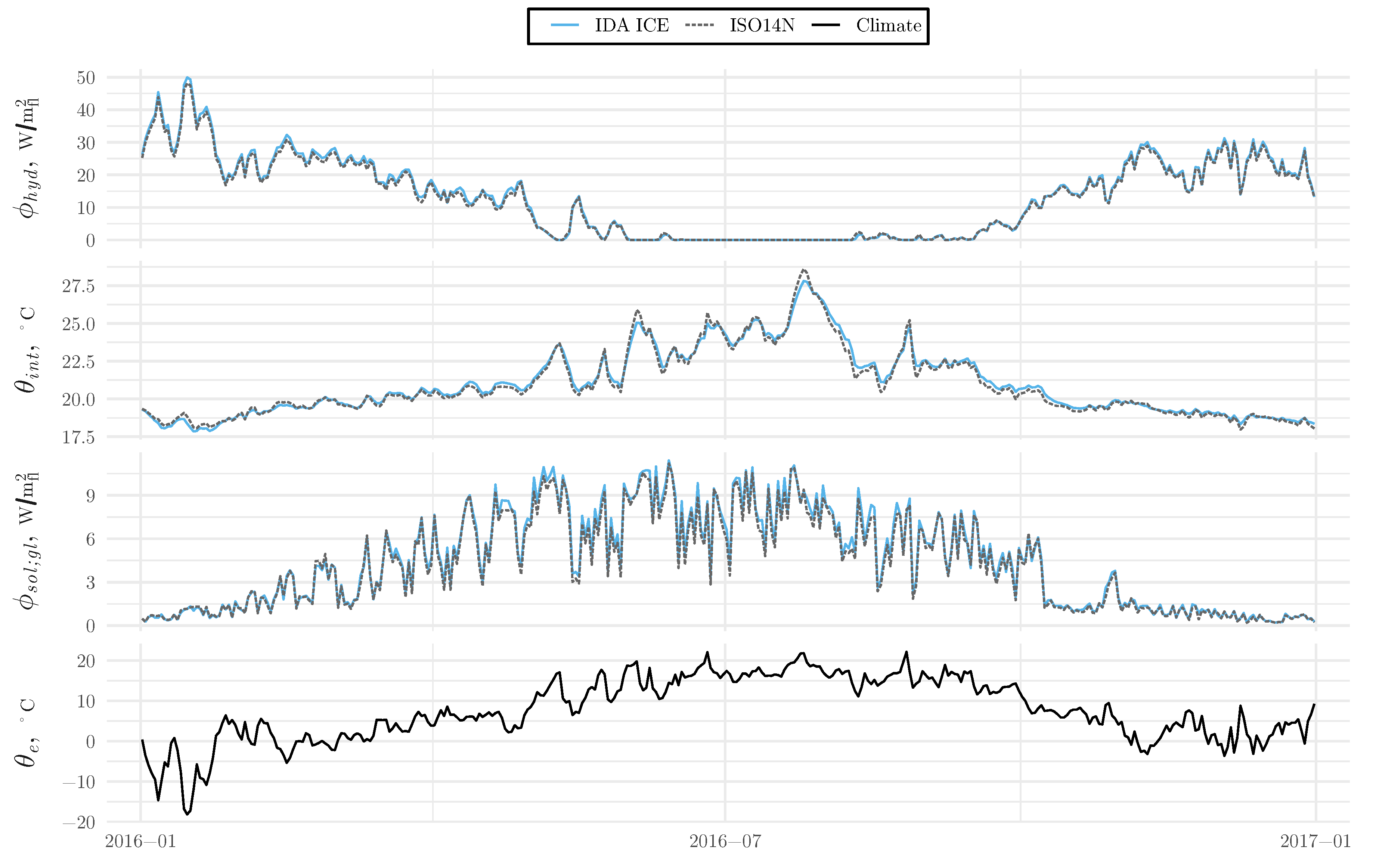
The heating system was modeled using the IDA ICE Water Radiator model (CeWatHet) with a nominal heat output of 50 W / m fl 2 (at a supply temperature of 60 C and a return at 40 C ), and the geometry of the radiator was set so that approximately half of the heat output was convective. The thermostatic control was modeled with a P-controller with a proportional band of 2 C , a time constant of 20 min, and the set-point set to 21 C . Table 4 shows the used look-up table for supply temperatures to the radiators. Ventilation was set to a constant 0.35 l / ( s · m fl 2 ) exhaust flow. Window blinds g-value was set to 0.53 and always fully drawn, internal heat gain was set to a constant of 3 W / m fl 2 , and thermal bridges were set to zero. Infiltration was nominally set to zero; however, for the case of studying the air infiltration (Section 5.4), the building envelope airtightness was set to 1 ACH at a 50 Pa pressure difference, and the surface pressure coefficient was semi-exposed.

5. Results

The developed ISO14N model and its procedures were validated by comparing it with simulations conducted with the detailed building energy simulation software IDA ICE.

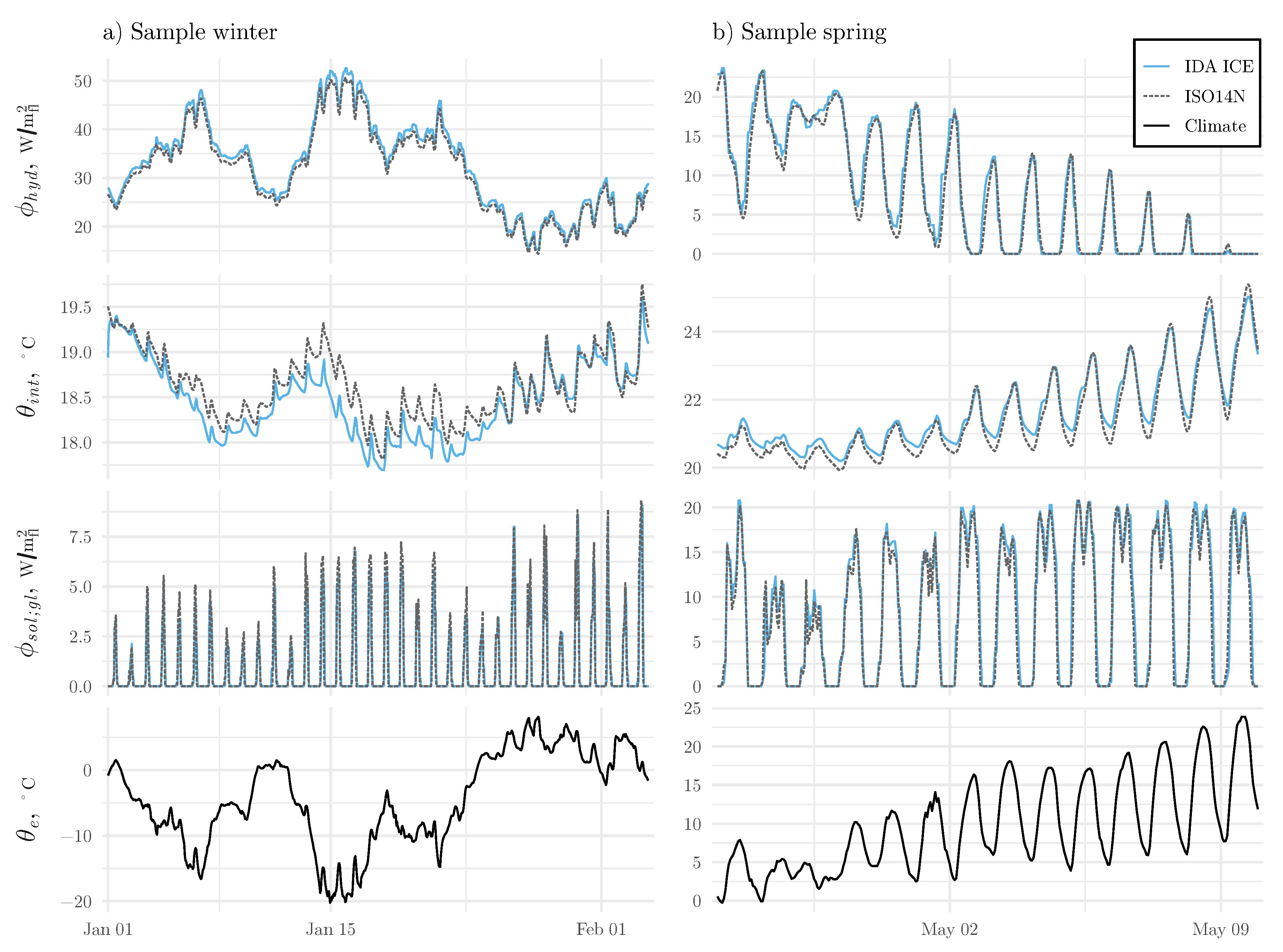
5.1. Full-Year Simulation Comparison with IDA ICE

In this section, simulation results from the developed ISO14N model are compared with results from an IDA ICE simulation. As seen in Figure 3, the ISO14N is capable of reproducing results of the detailed IDA ICE model (see Appendix B for comparisons on monthly and daily scales). The first half of January 2016 had two successive cold spells. During this period, the models show larger deviations, suggesting that they differ in thermal capacity behavior in the lower frequencies. A perfectly sized heating system would result in internal air temperature close to the set-point during the heating season. The heating system was on purpose undersized to cause more deviations from the set-point temperature, which makes differences in dynamical behavior more apparent. Table 6 shows the root mean square deviation (RMSD) [38] and the coefficient of variation (CV) of the RMSD [38], calculated on hourly, daily, and monthly averages. As can be seen from the table, the ISO14N is able to replicate simulation results of IDA ICE on an hourly basis, which is much more sensitive to dynamics than daily or monthly averages.

5.2. Node Temperature Profiles of External Wall Elements

For the developed ISO14N model, the external walls are represented by one element with three temperature nodes, while the IDA ICE model has four external wall elements (one in each cardinal direction) with five temperatures nodes each. For better comparability, the external wall temperatures of the IDA ICE model is averaged by node position. As seen in Figure 4, the node temperature profiles of the two models behave quite differently, which is mostly due to the different number of nodes and different approaches to distribute thermal properties between the nodes. Still, the estimated internal air temperatures match well.

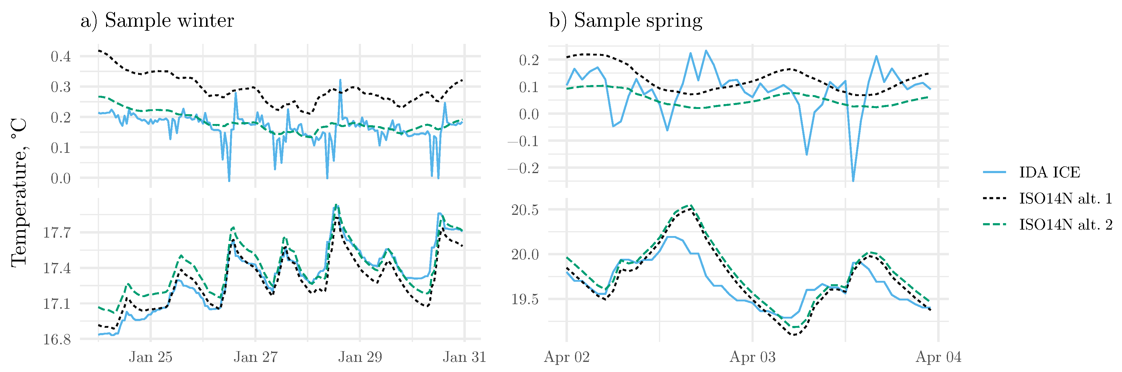
5.3. Operative Temperature

Operative temperature was calculated in two different ways and compared with output from IDA ICE. “ISO14N alt. 1” in Figure 5 was calculated according to Equation (18), while “ISO14N alt. 2” was calculated using Equation (19) with the weighting/conversion factor C h y d ; r ; m n (expressing the impact of the hydronic heating system) set to C h y d ; r ; m n = 0.02 . As seen in Figure 5, the operative temperature of “ISO14N alt. 1” deviates from the operative temperature acquired from IDA ICE, especially during cold weather, which was expected as IDA ICE weights in the surface temperatures of the radiator panels in the calculation of operative temperatures. Using Equation (19) and setting C h y d ; r ; m n = 0.02 results in a closer match. The C h y d ; r ; m n parameter could be derived from typical radiator panel configurations, but here it has been chosen by empirically matching it to the results of IDA ICE.
From Figure 5, it can be observed that IDA ICE appears to be more responsive to higher frequencies. This can partly be explained by the fact that IDA ICE splits the building elements into more nodes and uses surface nodes without mass. The other part of the explanation is that IDA ICE uses a fully dynamic simulation procedure (dynamic state transitions and variable heat transfer coefficients), while ISO14N linearizes the state transitions and uses constants for the interior surface heat transfer coefficients.

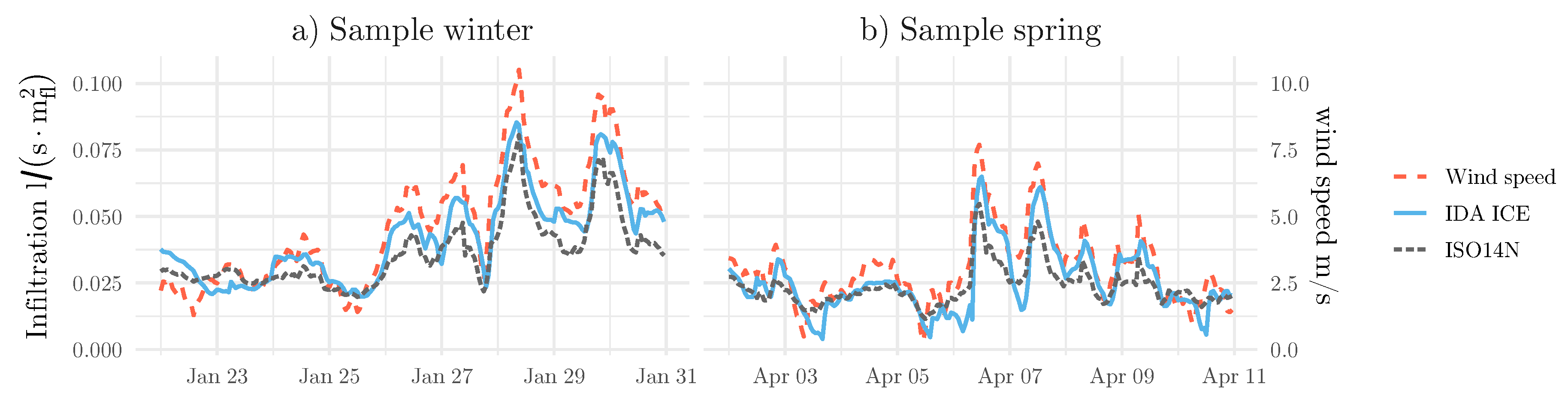
5.4. Air Infiltration

The air infiltration implementation described in Section 2.4 (with shelter class set to 3 and the flow coefficient set to C i n f = 0.08 l / ( s · Pa n · m fl 2 ) is here compared with output from IDA ICE. As seen in Figure 6, the implemented infiltration model produces similar results as the single-zone, one-floor-high, IDA ICE building model.

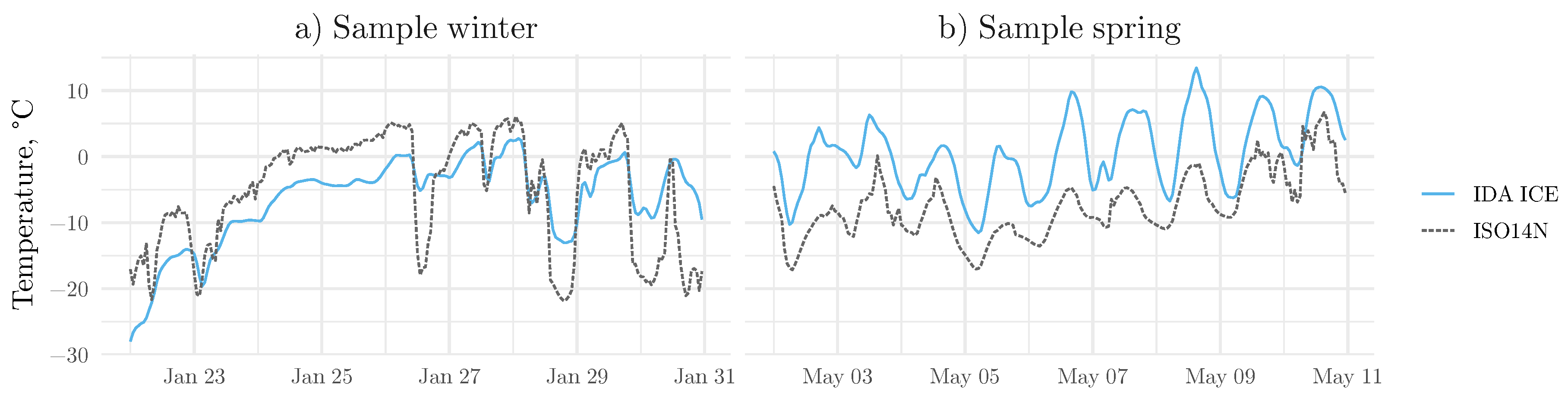
5.5. Sky Temperature and Thermal Radiation to the Sky

Apparent sky temperature was calculated from the ERA5 variable “surface thermal radiation downwards” using Equation (37) and compared to output from IDA ICE. In IDA ICE, the apparent sky temperature was empirically derived from dry and dew point temperatures and cloud cover using the Walton–Clark–Allen model [39]. As seen in Figure 7, the proposed apparent sky temperature calculation differs substantially from that of IDA ICE, resulting in an hourly RMSD of 5.5 C . Using the defaults suggested in the ISO 52016-1:2017 [10] standard, the extra thermal radiation to the sky variable ϕ s k y results in a constant of 45 W / m s 2 ; deriving ϕ s k y from the “surface thermal radiation downwards” variable of ERA5 (as proposed in Section 2.5), this constant varies between −15 and 295 W / m s 2 , with an average of 61 W / m s 2 for the used climate file.

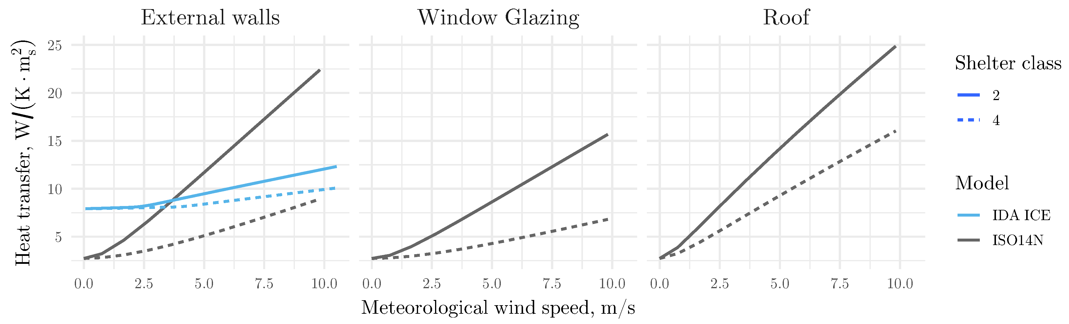
5.6. Exterior Surface Convective Heat Transfer Coefficients

Exterior surface convective heat transfer coefficients calculated according to Section 3.1 are presented and compared with IDA ICE. IDA ICE refers to Clarke [40] for its calculation procedure, a method that accounts for wind direction but does not distinguish between building element type. As seen in Figure 8, our Liu et al. [32]-based method results in the roof element being more sensitive to wind speed than other elements. The lower values for the glazing element, compared to the external walls, is explained by its surface roughness multiplier being set to smooth. IDA ICE’s method shows much less sensitivity to wind speed. For IDA ICE, the effect of wind direction is removed by showing smoothed lines of the average of the four external walls.

5.7. Shading Reduction Factor

Results of the proposed simplified shading calculation procedure (see Section 3.4) based on classification of the surrounding environment are presented. Table 7 shows the impact on annual solar irradiance received on vertical surfaces. The climate file described in Section 4 was used. The results can be compared to study conducted by Romero Rodríguez et al. [41], which showed an average of 35% reduction on solar irradiance for facades in the urban parts of Ludwigsburg. This part of the proposed modeling framework would benefit from further development, for example by employing aerial LiDAR data to model shading from the surrounding environment more accurately, see for example Lingfors et al. [17].

5.8. Window Blinds

Calculating the impact from window blinds according to Section 3.5, with the window blinds maximum g-value set to g b l ; m a x = 0.4 , results in a 30% reduction of annual solar heat gains through window glazing. According to Van Den Wymelenberg [33], there is no comprehensive consensus about how to model occupant-operated window blinds. Nonetheless, the proposed procedure is anticipated to model the impact from window blinds more accurately than for example using a constant value. IDA ICE uses an on/off controller, which controls the window blinds position as a function of the outside solar radiation level (100 W/m2 default set-point). This control scheme resulted in a 31% reduction of annual solar heat gains for the studied building and the climate file.

5.9. Computation Benchmark

This section show computation timings from conducted speed tests with the proposed ISO14N model, variants of it, and IDA ICE. The proposed ISO14N model pre-inversed its matrix A (the RC network) before the actual simulation run. For comparison, timing comparisons for model variants, where the matrix A of the RC network was inverted at each time-step, were also conducted. To compare speed in relation to a full ISO 52016-1:2017 implementation, an emulation was constructed and denoted “ISO41N” (due to its 41 temperature nodes). Table 8 shows the results. The largest speed gain was achieved from the matrix pre-inversion. Matrix inversion is computationally intensive and has a computation cost relationship of O( n 2 ). The use of a pre-inverted matrix A breaks the O( n 2 ) computational cost relationship and results in an approximately linear relationship between the RC network size and computation time. For the pre-inverted cases, it can be seen that the proposed simplification compared to a full ISO 52016-1:2017 implementation results in an approximately three-fold speed gain. The computation time difference between IDA ICE and the ISO14N is approximately 900 times (or an order of 1 magnitude).
The benchmark was conducted on a standard laptop computer with an Intel Core i7-7500U processor using one thread. All models were simulated using one year of climate, plus 14 days for the adaptation period. IDA ICE simulation was performed within the user interface, using initial default settings and all variable logging turned off; timing was conducted manually with a stopwatch. Various types of the ISO14N model used a calculation interval of 0.5 h (18,384 calculation time-steps in total), and logged and returned energy use and internal air temperature.

6. Discussion

It has been shown that the proposed ISO14N model was able to reproduce the hourly energy use pattern obtained with the detailed building energy simulation software IDA ICE. The use of a hydronic radiator heating system limits the application to mainly multifamily buildings in Nordic climates. However, the proposed RC network itself is generic and could probably replace a full ISO 52016-1:2017 implementation in other applications, such as generic energy need calculations or as a basis for energy use calculation for cooling.
In the development of the proposed ISO14N model, effort was made to achieve fast simulation times without a significant loss of accuracy. The optimization for computational efficiency is motivated by that calibration approaches typically use algorithmic differentiation which requires the model to be simulated several times (10k or more for Monte Carlo simulation approaches). Speed gains were achieved by moving parts of the calculation load to the pre-processing, i.e., model nodal reduction, and by a simulation procedure that uses pre-inverted matrices for the RC network. The proposed simplification of the RC network consists of lumping building elements by type and decreasing the number of temperature nodes in opaque building elements (see Figure 2), resulting in a system of 14 temperature nodes. The largest speed gain was achieved from pre-inverting the matrix A of the RC network, breaking the O( n 2 ) cost relationship and resulting in an approximately linear relationship between the RC network size and computation time. Pre-inversion requires the use of a constant matrix A element values, which results in a less flexible modeling structure. A constant A matrix, in turn, requires the use of node temperatures from the earlier time step for certain calculations (e.g., for the heating system control), which can result in time-shifts and numerical instabilities. However, our results show that the proposed ISO14N model achieves stable results without noticeable time-shifts.
During the development stage, a five-temperature node version (not included in this paper) was also tested and showed only limited performance gains compared to the proposed three-node version. Using five nodes adds flexibility and is likely to better model thermal admittance and more complex building structures such as sandwich walls (Akander [42]). However, for the intended use case of auto-generation of baseline models in large building stocks, it is anticipated that detailed information about construction will seldom be available in digital form. In the case of access to more detailed information, the proposed thermal network can be extended by adding more temperature nodes and/or by dividing the modeled building into more thermal zones.
Procedures to acquire and make use of satellite-based solar radiation data were presented, see Section 3.3. Solar radiation has a large impact on the thermal balance of buildings, and thermostatic radiators valves are often specifically used to avoid overheating due to solar heat gains. Thus, being able to model solar heat gains on an hourly basis (both directly through glazing and transmitted through opaque building elements) is anticipated to facilitate parameter estimation with hybrid/gray-box calibration methods. Reanalysis climate model data from ERA5 (see Section 4.2) was utilized. Conventional climate variables wind and air temperature were used as well as the more unconventional variables of ground temperature, ground albedo, and surface thermal radiation downward. Some of the benefits of using reanalysis data sources such as ERA5 are that the data are homogeneous and harmonized, covering the entire world, there is no need to deal with missing data, there is access to variables that are seldom measured locally, and the data are readily and publicly accessible. The temporal and spatial resolution of ERA5 is relatively rough, and in some cases it might be better to use local measurements (e.g., air temperature is readily measured locally at the building site).

7. Conclusions

A space heating model suitable for auto-generating baseline models of existing multifamily buildings has been proposed. As demonstrated in the result section, the proposed ISO14N model was able to reproduce the hourly energy use of space heating, indoor temperature, and operative temperature patterns obtained from the detailed building energy simulation software IDA ICE. Thus, the proposed model can be expected to model existing multifamily buildings, where space heating is provided by hydronic heating systems, to a similar degree of confidence as established simulation software.
The conducted computation timing showed that the proposed ISO14N was in the approximately 900 times faster than the detailed IDA ICE simulation. The largest speed gain was achieved from pre-inverting the matrix A of the RC network, resulting in an approximately linear cost relationship between the RC network size and computation time. Despite the use of constant pre-inverted A matrix, the proposed ISO14N model can achieve stable results without noticeable time-shifts. The achieved fast computation time enables using time-sensitive applications, such as Monte Carlo based calibration methods.
Solar heat gains have large impact on the thermal balance of buildings, and hydronic heating system often use thermostatic radiators valves to avoid overheating due to solar heat gains. Thus, it is necessary to model actual solar heat gains. We have presented procedures for converting sub-hourly satellite-based solar irradiation data to solar heat gains, while considering effects from building orientation, shading, and window blinds.
Future work will be conducted on calibrating the proposed model with actual energy meter readings, to ensure it represents the actual performance of the building and not only intended/designed performance. Hourly meter readings from district heating substations usually do not distinguish between domestic hot water and space heating. Thus, energy use for the occupant dependent domestic hot water needs to be modeled to be able to apply the proposed model on real buildings. Also, internal heat gains should be either measured (domestic electricity is always measured but not always readily available) or modeled to account for its occupant behavior dependent variations. The solar heat gain calculation could also be improved by employing aerial LiDAR data to model shading from the surrounding environment more accurately.

Supplementary Materials

The following are available online at https://www.mdpi.com/1996-1073/12/3/485/s1, Spreadsheet S1: Equation (11), empirical return temperature.

Author Contributions

For this article, the contributions of each author are listed as follows: L.L. contributed with conceptualization, coding, simulation, analysis, validation, and original draft preparation; J.A. contributed with knowledge, validation, and review and editing; J.Z. contributed with knowledge, validation, and review and editing.

Funding

The work was funded by Eskilstuna Kommunfastigheter, Eskilstuna Energy and Environment, and the Knowledge Foundation (KK-stiftelsen).

Acknowledgments

The work has been carried out under the auspices of the industrial post-graduate school Reesbe, and was funded by Eskilstuna Kommunfastigheter, Eskilstuna Energy and Environment, and the Knowledge Foundation (KK-stiftelsen).

Conflicts of Interest

The authors declare no conflict of interest.

Abbreviations

The following symbols are used in this manuscript:
α s o l solar absorption [-] or solar altitude [ ]
η efficiency [-]
γ azimuth angle [ ]
Δ t time interval [ h ]
κ areal heat capacity [ Wh / ( C · m s 2 ) ]
κ ρ a heat capacity of air per volume [ Ws / ( l · C ) ]
ϕ normalized thermal power [ W / m fl 2 ]
ρ a density of air [ kg / m 3 ]
σ Stefan-Boltzmann constant, 5.67e-8 [ W / ( m 2 · K 4 ) ]
θ centigrade temperature [ C ]
A , X , b square matrix of system coefficients, vector of unknown node temperatures, vector of known terms
Ccoefficient [-] or normalized heat capacity [ Wh / ( C · m fl 2 ) ]
D Data
D , H , L distance, height, length [ m ]
F , f factor/fraction [-]
Hnormalized heat transfer coefficient [ W / ( C · m fl 2 ) ]
H * modified building’s ceiling height [ m ]
Isolar or thermal radiation [ W / m s 2 ]
Qspecific air flow rate [ l / ( s · m fl 2 ) ]
Q * potential specific air flow rate [ Pa n / m fl 2 ]
Rnormalized thermal resistance [ m fl 2 · C /W]
Uthermal transmittance [ W / ( C · m s 2 ) ]
U l o c , U 10 m local wind speed [ m / s ], meteorological wind speed at 10 m height [ m / s ]
gtotal solar energy transmittance [-]
hsurface coefficient of heat transfer [ W / ( C · m s 2 ) ]
nexponent
rratio [-]
ucontrol signal [-]
The following subscripts are used in this manuscript:
bbuilding
b l (window) blinds
b o u boundary
c , c i convective, convective interior surface
ddesign (nominal)
d i f , d i r diffuse, direct
eexternal (as in outdoor)
e l (building) element
e n v environment
e w external walls
g f ground floor
g l glazing (windows, doors etc)
g r ground
h o r horizontal
h y d hydronic heating system
i m internal mass (internal walls, intermediate floors and adiabatic external walls)
i n f infiltration (uncontrolled air leakage)
i n t internal (as in indoor)
l m t d radiator logarithmic mean temperature difference
mmass related conductance or capacitance
m a x maximum
o b s t , o v h obstacle, overhang
p b proportional band
r , r i radiative, radiative interior surface
r e t return
r f roof
sstack
s e , s i surface exterior, surface interior
s e t set-point
s h shading or sheltering
s k y sky temperature or sky thermal radiation
s o l solar radiation/heat gain
s t r d surface thermal radiation downwards
s u p supply
s y s system
t time index
t b thermal bridges
t o t total
t r v thermostatic radiator valve(s)
v e ventilation
v e r vertical
v i virtual ground layer
wwind
w m a weighted moving average

Appendix A. Construct of the Linear Equations System

A = A 1 H 1 ; r f 0 0 0 0 0 0 0 0 0 0 0 0 H 1 ; r f A 2 H 2 ; r f 0 0 0 0 0 0 0 0 0 0 0 0 H 2 ; r f A 3 0 0 f e w · H r i ; r f 0 f g l · H r i ; r f 0 f i m · H r i ; r f 0 0 f g f · H r i ; r f H c i ; r f 0 0 0 A 4 H 1 ; e w 0 0 0 0 0 0 0 0 0 0 0 0 H 1 ; e w A 5 H 2 ; e w 0 0 0 0 0 0 0 0 0 0 f r f · H r i ; e w 0 H 2 ; e w A 6 0 f g l · H r i ; e w 0 f e w · H r i ; e w 0 0 f g f · H r i ; e w H c i ; e w 0 0 0 0 0 0 A 7 H 1 ; g l 0 0 0 0 0 0 0 0 f r f · H r i ; g l 0 0 f e w · H r i ; g l H 1 ; g l A 8 0 f i m · H r i ; g l 0 0 f g f · H r i ; g l H c i ; g l 0 0 0 0 0 0 0 0 A 9 H 1 ; i m 0 0 0 0 0 0 f r f · H r i ; i m 0 0 f e w · H r i ; i m 0 f g l · H r i ; i m H 1 ; i m A 10 0 0 f g f · H r i ; i m H c i ; i m 0 0 0 0 0 0 0 0 0 0 A 11 H 1 ; g f 0 0 0 0 0 0 0 0 0 0 0 0 H 1 ; g f A 12 H 2 ; g f 0 0 0 f r f · H r i ; g f 0 0 f e w · H r i ; g f 0 f g l · H r i ; g f 0 f i m · H r i ; g f 0 H 2 ; g f A 13 H c i ; g f 0 0 H c i ; r f 0 0 H c i ; e w 0 H c i ; g l 0 H c i ; i m 0 0 H c i ; g f A 14
b T = b 1 , , b 14 , X T = θ 1 ; r f θ 2 ; r f θ 3 ; r f θ 1 ; e w θ 2 ; e w θ 3 ; e w θ 1 ; g l θ 2 ; g l θ 1 ; i m θ 2 ; i m θ 1 ; g f θ 2 ; g f θ 3 ; g f θ i n t
where the A 1 , , A 14 elements of matrix A and the b 1 , , b 14 elements of matrix b are detailed in Table A1 and Table A2 respectively.
Table A1. Elements A 1 , , A 14 of matrix A . e l refers to the five building element types.
el Exterior Surface NodesInside NodesInterior Surface Nodes
r f A 1 = C 1 ; r f Δ t + H 1 ; r f + H s e ; r f ; t A 2 = C 2 ; r f Δ t + H 2 ; r f + H 1 ; r f A 3 = C 3 ; r f Δ t + H c i ; r f + ( 1 f r f ) · H r i ; r f + H 2 ; r f
e w A 4 = C 1 ; e w Δ t + H 1 ; e w + H s e ; e w ; t A 5 = C 2 ; e w Δ t + H 2 ; e w + H 1 ; e w A 6 = C 3 ; e w Δ t + H c i ; e w + ( 1 f e w ) · H r i ; e w + H 2 ; e w
g l A 7 = H 1 ; g l + H s e ; g l ; t A 8 = H c i ; g l + ( 1 f g l ) · H r i ; g l + H 1 ; g l
i m A 9 = C 1 ; i m Δ t + H 1 ; i m A 10 = C 2 ; i m Δ t + H c i ; i m + ( 1 f i m ) · H r i ; i m + H 1 ; i m
g f A 11 = C 1 ; g f Δ t + H s e ; g f + H 1 ; g f A 12 = C 2 ; g f Δ t + H 2 ; g f + H 1 ; g f A 13 = C 3 ; g f Δ t + H c i ; g f + ( 1 f g f ) · H r i ; g f + H 2 ; g f
Internal air node:
A 14 = C i n t Δ t + H c i ; r f + H c i ; e w + H c i ; g l + H c i ; i m + H c i ; g f + H t b
Table A2. Elements b 1 , , b 14 of matrix b . e l refers to the five building element types.
el Exterior Surface NodesInside NodesInterior Surface Nodes
r f b 1 = C 1 ; r f Δ t · θ 1 ; r f ; t 1 + H s e ; r f ; t · θ e ; t + ϕ r e ; r f ; t b 2 = C 2 ; r f Δ t · θ 2 ; r f ; t 1 b 3 = C 3 ; r f Δ t · θ 3 ; r f ; t 1 + ϕ r i ; r f ; t
e w b 4 = C 1 ; e w Δ t · θ 1 ; e w ; t 1 + H s e ; e w ; t · θ e ; t + ϕ r e ; e w ; t b 5 = C 2 ; e w Δ t · θ 2 ; e w ; t 1 b 6 = C 3 ; e w Δ t · θ 3 ; e w ; t 1 + ϕ r i ; e w ; t
g l b 7 = H s e ; g l ; t · θ e ; t + ϕ r e ; g l ; t b 8 = ϕ r i ; g l ; t
i m b 9 = C 1 ; i m Δ t · θ 1 ; i m ; t 1 b 10 = C 2 ; i m Δ t · θ 2 ; i m ; t 1 + ϕ r i ; i m ; t
g f b 11 = C 1 ; g f Δ t · θ 1 ; g f ; t 1 + H s e ; g f · θ g r ; t b 12 = C 2 ; g f Δ t · θ 2 ; g f ; t 1 b 13 = C 3 ; g f Δ t · θ 3 ; g f ; t 1 + ϕ r i ; g f ; t
Internal air node:
b 14 = C i n t Δ t · θ i n t ; t 1 + H t b · θ e ; t ϕ v e ; t ϕ i n f ; t + f c ; i n t · ϕ i n t ; t + f c ; s o l · ϕ s o l ; t + f c ; h y d · ϕ h y d ; t

Appendix B. Full-Year Comparison

Table A3. Energy use for space heating as monthly sums and deviations between the models.
MonthIDA ICE, kWh / m fl 2 ISO14N, kWh / m fl 2 Deviation, kWh / m fl 2 Deviation, %
124.823.90.93.6%
217.917.20.74.1%
315.414.70.74.5%
410.09.30.76.9%
53.02.90.14.3%
60.10.10.0-
70.00.00.0-
80.30.4-0.1-
91.51.50.00.8%
1010.710.40.33.0%
1116.716.20.53.1%
1217.817.20.52.9%
Sum118.3114.04.43.7%
Figure A1. Full-year comparison with IDA ICE, using daily average values: energy use for space heating, ( ϕ h y d ), internal air temperature ( θ i n t ), solar heat gains through glazing ( ϕ s o l ; g l ) and external air temperature ( θ e ).
Energies 12 00485 g0a1

References

  1. Coakley, D.; Raftery, P.; Keane, M. A review of methods to match building energy simulation models to measured data. Renew. Sustain. Energy Rev. 2014, 37, 123–141. [Google Scholar] [CrossRef]
  2. Ciancio, V.; Falasca, S.; Golasi, I.; Curci, G.; Coppi, M.; Salata, F. Influence of Input Climatic Data on Simulations of Annual Energy Needs of a Building: EnergyPlus and WRF Modeling for a Case Study in Rome (Italy). Energies 2018, 11, 2835. [Google Scholar] [CrossRef]
  3. ASHRAE. ASHRAE Handbook—Fundamentals (SI Edition); ASHRAE: Atlanta, GA, USA, 2017. [Google Scholar]
  4. EnergyPlus. EnergyPlus 8.9 Documentation—Engineering Reference; Technical Report; U.S. Department of Energy: Washington, DC, USA, 2018.
  5. Kang, Y.; Krarti, M. Bayesian-Emulator based parameter identification for calibrating energy models for existing buildings. Build. Simul. 2016, 9, 411–428. [Google Scholar] [CrossRef]
  6. Tian, W.; Yang, S.; Li, Z.; Wei, S.; Pan, W.; Liu, Y. Identifying informative energy data in Bayesian calibration of building energy models. Energy Build. 2016, 119, 363–376. [Google Scholar] [CrossRef]
  7. Amasyali, K.; El-Gohary, N.M. A review of data-driven building energy consumption prediction studies. Renew. Sustain. Energy Rev. 2018, 81, 1192–1205. [Google Scholar] [CrossRef]
  8. Bacher, P.; Madsen, H. Identifying suitable models for the heat dynamics of buildings. Energy Build. 2011, 43, 1511–1522. [Google Scholar] [CrossRef] [Green Version]
  9. Boodi, A.; Beddiar, K.; Benamour, M.; Amirat, Y.; Benbouzid, M. Intelligent Systems for Building Energy and Occupant Comfort Optimization: A State of the Art Review and Recommendations. Energies 2018, 11, 2604. [Google Scholar] [CrossRef]
  10. ISO. ISO 52016-1:2017—Energy Performance of Buildings—Energy Needs for Heating and Cooling, Internal Temperatures and Sensible and Latent Heat Loads—Part 1: Calculation Procedures (ISO 52016-1:2017); ISO: Geneva, Switzerland, 2017. [Google Scholar]
  11. ISO. ISO 13790:2008—Energy Performance of Buildings—Calculation of Energy Use For Space Heating and Cooling (ISO 13790:2008); ISO: Geneva, Switzerland, 2008. [Google Scholar]
  12. Pavlak, G.S.; Florita, A.R.; Henze, G.P.; Rajagopalan, B. Comparison of Traditional and Bayesian Calibration Techniques for Gray-Box Modeling. J. Archit. Eng. 2014, 20, 04013011. [Google Scholar] [CrossRef]
  13. Piotr, M. The simple hourly method of EN ISO 13790 standard in Matlab/Simulink: A comparative study for the climatic conditions of Poland. Energy 2014, 75, 568–578. [Google Scholar]
  14. Fischer, D.; Wolf, T.; Scherer, J.; Wille-Haussmann, B. A stochastic bottom-up model for space heating and domestic hot water load profiles for German households. Energy Build. 2016, 124, 120–128. [Google Scholar] [CrossRef]
  15. Vivian, J.; Zarrella, A.; Emmi, G.; De Carli, M. An evaluation of the suitability of lumped-capacitance models in calculating energy needs and thermal behaviour of buildings. Energy Build. 2017, 150, 447–465. [Google Scholar] [CrossRef]
  16. Wang, R. 3D building modeling using images and LiDAR: A review. Int. J. Image Data Fusion 2013, 4, 273–292. [Google Scholar] [CrossRef]
  17. Lingfors, D.; Bright, J.; Engerer, N.; Ahlberg, J.; Killinger, S.; Widén, J. Comparing the capability of low- and high-resolution LiDAR data with application to solar resource assessment, roof type classification and shading analysis. Appl. Energy 2017, 205, 1216–1230. [Google Scholar] [CrossRef]
  18. Gadd, H.; Werner, S. Fault detection in district heating substations. Applied Energy 2015. [Google Scholar] [CrossRef]
  19. Werner, S. District heating and cooling in Sweden. Energy 2017, 126, 419–429. [Google Scholar] [CrossRef]
  20. Energy in the Buildings—Technical Properties and Calculations—Results from Project BETSI; Technical Report; Swedish National Board of Housing, Building and Planning (Boverket): Stockholm, Sweden, 2010.
  21. Olsson, D. Modellbaserad Styrning av Värmesystem Baserat på Prognostiserat väder Modellbaserad Styrning av Värmesystem Baserat på Prognostiserat Väder. Ph.D. Thesis, Chalmers University of Technology, Göteborg, Sweden, 2014. [Google Scholar]
  22. Jangsten, M.; Kensby, J.; Dalenbäck, J.O.; Trüschel, A. Survey of radiator temperatures in buildings supplied by district heating. Energy 2017, 137, 292–301. [Google Scholar] [CrossRef] [Green Version]
  23. Carpenter, B.; Gelman, A.; Hoffman, M.; Lee, D.; Goodrich, B.; Betancourt, M.; Brubaker, M.; Guo, J.; Li, P.; Riddell, A. Stan: A Probabilistic Programming Language. J. Stat. Softw. 2017, 76, 1–32. [Google Scholar] [CrossRef] [Green Version]
  24. Wickham, H.; François, R.; Henry, L.; Müller, K. Dplyr: A Grammar of Data Manipulation; R Package Version 0.7.8. 2018. Available online: https://libraries.io/cran/dplyr (accessed on 2 February 2019).
  25. ISO. ISO 52010:2017—Energy Performance of Buildings—External Climatic Conditions—Part 1: Conversion of Climatic Data for Energy Calculations (EN ISO 52010:2017); ISO: Geneva, Switzerland, 2017. [Google Scholar]
  26. ISO. ISO 13370:2017—Thermal Performance of Buildings—Heat Transfer via the Ground—Calculation Methods (ISO 13370:2017); ISO: Geneva, Switzerland, 2017. [Google Scholar]
  27. Walker, I.S.; Wilson, D.J. Field Validation of Algebraic Equations for Stack and Wind Driven Air Infiltration Calculations. HVAC&R Res. 1998, 4, 119–139. [Google Scholar] [CrossRef] [Green Version]
  28. Wang, W.; Beausoleil-Morrison, I.; Reardon, J. Evaluation of the Alberta air infiltration model using measurements and inter-model comparisons. Build. Environ. 2009, 44, 309–318. [Google Scholar] [CrossRef]
  29. Hayati, A.; Mattsson, M.; Sandberg, M. Evaluation of the LBL and AIM-2 air infiltration models on large single zones: Three historical churches. Build. Environ. 2014, 81, 365–379. [Google Scholar] [CrossRef]
  30. Jokisalo, J.; Kurnitski, J.; Korpi, M.; Kalamees, T.; Vinha, J. Building leakage, infiltration, and energy performance analyses for Finnish detached houses. Build. Environ. 2009, 44, 377–387. [Google Scholar] [CrossRef]
  31. Mirsadeghi, M.; Cóstola, D.; Blocken, B.; Hensen, J.L.M. Review of external convective heat transfer coefficient models in building energy simulation programs: Implementation and uncertainty. Appl. Therm. Eng. 2013, 56, 134–151. [Google Scholar] [CrossRef]
  32. Liu, J.; Heidarinejad, M.; Gracik, S.; Srebric, J. The impact of exterior surface convective heat transfer coefficients on the building energy consumption in urban neighborhoods with different plan area densities. Energy Build. 2015, 86, 449–463. [Google Scholar] [CrossRef]
  33. Van Den Wymelenberg, K. Patterns of occupant interaction with window blinds: A literature review. Energy Build. 2012. [Google Scholar] [CrossRef]
  34. Sandberg, E.; Engvall, K. Delrapport 3 (MEBY): Beprövad Enkät-Hjälpmedel för Energiuppföljning; Technical Report; MEBY: Stockholm, Sweden, 2002. [Google Scholar]
  35. Hoyer-Klick, C.; Lefèvre, M.; Schroedter-Homscheidt, M.; Wald, L. MACC-III Deliverable D57.5: USER’ S GUIDE to the MACC-RAD Services on Solar Energy Radiation Resources; Technical Report: Copernicus, European Union’s Earth Observation Programme; 2015; Available online: https://www.researchgate.net/publication/281150019_USER’S_GUIDE_to_the_MACC-RAD_Services_on_solar_energy_radiation_resources_March_2015 (accessed on 2 February 2019).
  36. Hersbach, H.; Dick, D. ERA5 reanalysis is in production. ECMWF Newsl. 2016, 147, 7. [Google Scholar]
  37. Lundström, L.; Wallin, F. Heat demand profiles of energy conservation measures in buildings and their impact on a district heating system. Appl. Energy 2016, 161, 290–299. [Google Scholar] [CrossRef] [Green Version]
  38. Ruiz, G.; Bandera, C. Validation of Calibrated Energy Models: Common Errors. Energies 2017, 10, 1587. [Google Scholar] [CrossRef]
  39. Walton, G. Thermal Analysis Research Program Reference Manual-NBSSIR 83-2655; Technical Report; National Bureau of Standards: Washington, DC, USA, 1983.
  40. Clarke, J.A. Energy Simulation in Building Design; Adam Hilger Lt: Bristol, UK, 1985. [Google Scholar]
  41. Romero Rodríguez, L.; Nouvel, R.; Duminil, E.; Eicker, U. Setting intelligent city tiling strategies for urban shading simulations. Sol. Energy 2017, 157, 880–894. [Google Scholar] [CrossRef]
  42. Akander, J. The ORC Method—Effective Modelling of Thermal Performance of Multilayer Building Components. Ph.D. Thesis, Royal Institute of Technology, Stockholm, Sweden, 2000. [Google Scholar]
Figure 1. Process from data input (a) to pre-processing (b) and to the simulation procedure (c).
Energies 12 00485 g001
Figure 2. An RC network representation of the proposed ISO14N model.
Energies 12 00485 g002
Figure 3. Hourly output variable comparison with IDA ICE. Diagram panels in column (a) shows a winter sample period, column (b) shows a spring sample period. Diagram panel rows compare following variables: energy use for space heating ( ϕ h y d ), internal air temperature ( θ i n t ), solar heat gains through glazing ( ϕ s o l ; g l ), and external air temperature ( θ e ).
Energies 12 00485 g003
Figure 4. Comparison with IDA ICE on node temperatures for external walls. Diagram panels in column (a) shows a winter sample period, column; (b) shows a spring sample period. Diagram panel rows, from uppermost to lowermost: internal air nodes; interior surface nodes; inside nodes (one for ISO14N and three for IDA ICE); exterior surface nodes; and external air temperature.
Energies 12 00485 g004
Figure 5. Comparison with IDA ICE on operative temperatures for two sample periods. The bottom row shows operative temperatures ( θ o p ) and the upper row shows the temperature difference between internal air temperature and operative temperatures ( θ i n t θ o p ).
Energies 12 00485 g005
Figure 6. Comparison with IDA ICE on air infiltration. The solid blue line shows an infiltration level from IDA ICE, a gray-dotted line shows an infiltration level from the ISO14N model, and the dashed red line shows the meteorological wind speed (scale on right-hand y-axis).
Energies 12 00485 g006
Figure 7. Comparison with IDA ICE on apparent sky temperatures for two sample periods. Solid blue line shows results from IDA ICE, gray dotted line shows from the ISO14N model.
Energies 12 00485 g007
Figure 8. Exterior surface convective heat transfer coefficients calculated for two sheltering classes.
Energies 12 00485 g008
Table 1. Node heat capacity distribution for the the 3-node building elements roof r f and external walls e w . Class I: concentrated on interior side; Class E: concentrated on exterior side; Class IE: divided on interior and exterior side; Class D: equally distributed; Class M: inside/centered.
NodeClass IClass EClass IEClass DClass M
10.100.500.400.330.10
20.400.400.200.330.80
30.500.100.400.330.10
Table 2. Plan area densities λ p [32], wind sheltering factors λ w [3], and solar shielding factors λ s o l for five shelter classes: ranging from (1) no shelter to (5) a highly dense urban area (neighboring buildings closer than one building height).
Shelter Class12345
λ p 0.000.040.110.250.44
λ w 1.000.900.700.500.30
λ s o l 3.002.501.901.300.70
Table 3. Environmental variables derived from ERA5. The ISO14N column shows variable names as they are used in this paper, while the ERA5 column shows the variables sourced from ERA5 according to the notation convention of ERA5.
DescriptionISO14NERA5Transformation
External air temperature at 2 m θ e 2 t Kelvin to centigrade
Ground temperature at 1.0–2.89 m θ g r s t l 4 Kelvin to centigrade
Wind speed at 10 m U 10 m 10 u , 10 v U 10 m = 10 u 2 + 10 v 2
Ground albedo α g r s s r , s s r d α g r = 1 s s r / s s r d
Surface thermal radiation downwards ϕ s t r d s t r d Joule to Watt-hours
Table 4. Supply temperature look-up table, used for both IDA ICE and ISO14N models.
θ e [ C ]−2001218
θ h y d ; s u p ; s e t [ C ]60432818
Table 5. Parameter input values used for the ISO14N model simulation.
ParameterDescriptionValue(s)Unit
N f l Number of floors1-
H f l Floor height2.6 m
PBuilding perimeter60 m
A f l Floor area2.6 m fl 2
γ Azimuth angles for the external walls[0, 90, −90, 180]
F γ Surface area fraction for the external walls[0.17, 0.33, 0.33, 0.17]-
r g l Glazing to floor ratio0.15-
g g l Solar transmittance of the glazing0.76-
g b l Solar transmittance of the window blinds0.53-
U r f Thermal transmittance of the roof0.20 W / ( C · m s 2 )
U e w Thermal transmittance of the external walls0.72 W / ( C · m s 2 )
U g l Thermal transmittance of the glazing2.9 W / ( C · m s 2 )
U g f Thermal transmittance of the ground floor0.23 W / ( C · m s 2 )
κ m ; r f Areal heat capacity of the external walls56 Wh / ( C · m s 2 )
κ m ; e w Areal heat capacity of the external walls15 Wh / ( C · m s 2 )
κ m ; g f Areal heat capacity of the external walls56 Wh / ( C · m s 2 )
Q v e Specific air flow rate of the ventilation system0.35 l / ( s · m fl 2 )
η v e Efficiency of the ventilation heat recovery0.0-
C i n f Normalized infiltration coefficient0.0 l / ( s · Pa n · m fl 2 )
H h y d Radiator constant, normalized per floor area0.66 W / ( C · m fl 2 )
θ i n t ; s e t Internal air set-point temperature21.0 C
H t b Heat transfer due to thermal bridges0.0 W / ( C · m fl 2 )
ϕ i n t Internal heat gains3.0 W / ( m fl 2 )
Δ t Calculations interval0.5
Table 6. Root mean square deviation (RMSD) for hourly, daily, and monthly averages on energy use ( ϕ h y d ) and internal air ( θ i n t ) and operative temperatures ( θ o p ) variables. For ϕ h y d , CV(RMSD) is shown within parenthesis.
VariableHourlyDailyMonthly
ϕ h y d , W / m fl 2 0.94 (2.6%)0.74 (2.0%)0.68 (1.8%)
θ i n t , C 0.300.260.17
θ o p , C 0.340.280.19
Table 7. Annual reduction of total solar irradiance on vertical surfaces, per sheltering class and building height.
Shading Class1122334455
Building height, m186186186186186
Annual solar reduction, %691117192829403849
Table 8. Computation benchmark, timing in milliseconds.
Model (Variant)Computation Time, ms
ISO14N (matrix pre-inverted)19
ISO41N (matrix pre-inverted)56
ISO14N (matrix inversion each time-step)83
ISO41N (matrix inversion each time-step)755
IDA ICE18,000

