A Data-Driven Approach for Enhancing the Efficiency in Chiller Plants: A Hospital Case Study
by
 , , , , and
Serafín Alonso
* ,
,
Antonio Morán
 ,
,
Miguel Ángel Prada
,
Perfecto Reguera
,
Juan José Fuertes
and
Manuel Domínguez
Grupo de Investigación en Supervisión, Control y Automatización de Procesos Industriales (SUPPRESS), Esc. de Ing. Industrial e Informática, Universidad de León, Campus de Vegazana s/n, 24007 León, Spain
*
Author to whom correspondence should be addressed.
Energies 2019, 12(5), 827; https://doi.org/10.3390/en12050827
Submission received: 14 January 2019
/
Revised: 14 February 2019
/
Accepted: 26 February 2019
/
Published: 2 March 2019
(This article belongs to the Special Issue Energy Performance and Indoor Climate Analysis in Buildings)
Abstract
:Large buildings cause more than 20% of the global energy consumption in advanced countries. In buildings such as hospitals, cooling loads represent an important percentage of the overall energy demand (up to 44%) due to the intensive use of heating, ventilation and air conditioning (HVAC) systems among other key factors, so their study should be considered. In this paper, we propose a data-driven analysis for improving the efficiency in multiple-chiller plants. Coefficient of performance (COP) is used as energy efficiency indicator. Data analysis, based on aggregation operations, filtering and data projection, allows us to obtain knowledge from chillers and the whole plant, in order to define and tune management rules. The plant manager software (PMS) that implements those rules establishes when a chiller should be staged up/down and which chiller should be started/stopped according different efficiency criteria. This approach has been applied on the chiller plant at the Hospital of León.

1. Introduction
Energy consumption in large buildings, such as hotels, museums, hospitals, commercial buildings, etc., represents more than 20% of the global energy consumption in developed countries [1]. The reasons behind such a high consumption are the addition of new building services, the increase of comfort levels, the additional time spent by people inside buildings, and the proliferation of heating, ventilation and air conditioning (HVAC) systems, among others [2]. Four types of energy consumption can be distinguished in those buildings: electricity, heating, hot water, and cooling [3]. Cooling loads usually have a seasonal behaviour and, in some buildings, they are not the most noteworthy, so their study is often disregarded. Cooling loads, however, represent an important percentage of the overall energy demand (up to 44%) in utility buildings with special facilities, such as hospitals [4]. For instance, hospitals keep a minimum level of cooling load during the whole year to guarantee the operation of hospital services: refrigeration of surgeries, scanners, magnetic resonance imaging systems and data centers, among other key facilities. Furthermore, cooling loads have a direct influence on the electricity demand, since chillers and their auxiliary elements (pumps, fans, cooling towers, etc.) are electric systems [4]. Therefore, both cooling load and chiller performance should be considered and analyzed in large buildings, in order to achieve energy efficiency. Additionally, many buildings require a reliable and secure cooling supply, so aspects such as monitoring, automatic management and assets maintenance play also an important role [5].
To achieve energy efficiency in a multiple-chiller plant, it is recommended to study, first, the individual chiller performance and, later, the overall plant performance [6]. The building management systems (BMS) acquire and store a great amount of real data, which can be analyzed and exploited to extract the implicit knowledge. So far, the vast amount of data was rarely translated into useful knowledge about potential energy performance improvements, due to its extreme complexity or a lack of effective data analysis techniques [7]. However, the novel advances in the data science allow us to address a complex data analysis.
Therefore, a data-driven analysis should be carried out in order to acquired knowledge about the plant [8]. The implicit knowledge which is discovered (analyzing past data from the chillers, from the whole plant and from the environment) can be added to the management strategies. It can be converted into rules to be used in an expert module with the final aim of enhancing energy efficiency [9]. A periodic data analysis of the chiller plant can help us to achieve a better understanding and to monitor efficiency, aiming to upgrade and tune the management rules and to implement more efficient up/down sequencing strategies.
The contribution of this paper is the proposal of a comprehensive methodology for improving the efficiency in multiple-chiller plants. This methodology is based on a data analysis of the operation of the chillers and the overall plant, using real data instead of simulations. The proposed data analyses highlight relevant information by applying aggregation, filtering and data projection. Using the knowledge extracted specifically from the plant, control parameters of the chillers can be adjusted and management rules can be defined or tuned. The aim is to achieve an efficient management of the plant, without the need of incorporating cutting-edge controllers, since the management rules obtained through the proposed approach can be easily deployed in existing controllers. The proposed approach is applied on the real chiller plant at the Hospital of León.
This paper is structured as follows: Section 2 reviews the previous related work. The data-driven approach to improve energy efficiency in chiller plants is proposed in Section 3. Then, the multiple-chiller plant at the Hospital of León is described in detail in Section 4. Section 5 explains the application of proposed methodology to that plant. Next, results on chiller and plant efficiencies are presented in Section 6. Finally, conclusions are drawn in Section 7.
2. Related Work
Reviewing the literature, some examples of research on data mining for improving energy efficiency in buildings can be found. These works focus on the use of data mining techniques to extract relationships and patterns of interest from a large dataset [7]. However, many works rely on simulations, using software as TRNSYS, EnergyPlus, etc. [10]. Data analytics on a detailed measured building performance can help us to identify and estimate energy savings and then to inform the decision making system [11].
Other research focuses on the use of machine learning techniques for forecasting the energy efficiency and consumption in the building and, afterwards, comparing the predicted values with the nominal ones in order to detect possible deviations [12]. Simulated data are generally based on a physical model of the system, often used to build prediction models [13]. On the other hand, prediction models of the HVAC systems have been also built using real data [14]. The third type of approach found in the literature is a grey box model, which merges the qualities of both the physics-based and data-driven models [15].
With regard to the measurement of energy efficiency, several indicators (EEI) can be used in the data analysis [16], ranging from the COP (Coefficient of Performance) or EER (Energy Efficiency Ratio) to more sophisticated indicators such as SCOP (Seasonal Coefficient of Performance), SEER (Seasonal Energy Efficiency Ratio) and IPLV (Integrated Part Load Value), which consider seasonal chiller operations and capacity modulation. Other research defines and uses specific EEIs [9]. Nevertheless, the computation of COP is quite simple from measurements of electricity consumption and cooling load, so this indicator is often used to characterize the chiller efficiency and the overall performance (including the performance of chillers, pumps, fans, refrigeration towers, etc.) [6]. The COP value depends on the chiller technology and on the surrounding conditions [17,18,19].
Smart buildings should incorporate the feedback from the data analysis in the management and control system in order to optimize the use of energy in different conditions [20,21]. The structure of the control system is usually based on a hierarchical multilevel concept [22,23], with a coordinator layer over the local control units. For instance, a hierarchical cascade control strategy for energy management of intelligent buildings is used in [24]. The plant management software (PMS) is in charge of operating the plant (together with the BMS) with the minimum energy consumption. For that, PMS implements efficient chiller sequencing strategies which decide when a chiller should be staged up/down and which chiller should be started/stopped, considering a cooling load, weather conditions, chiller load capacities, etc. [25,26,27]. Note that reducing condensing temperature leads also to an increase of the chiller performance [28,29]. The aim of the PMS is to maximize the overall COP, by adjusting the capacity of the plant to the fluctuating cooling load. Therefore, a PMS becomes essential to improve energy efficiency in multiple-chiller plants [30].
Most PMSs rely on complex optimization methods [31,32,33], which require a high computational effort and make the deployment on existing controllers so difficult that often the rules of these PMSs can be only tested on simulated plants. Other commercial software uses relational control, based on the equal marginal performance principle [34]. The aim of relational control is to achieve optimal energy efficiency of the plant, requiring each chiller to be operated in relation to the operation of the others.
Rule-based management strategies, together with performance monitoring tools and model-based predictive control, have been outlined as outstanding methods for intelligent HVAC control to enhance energy efficiency [35]. Rule-based management enables the translation of best practices, experience and knowledge of HVAC control engineers into a set of rules, which can be applied to operate the plant. Other control methods and optimization techniques developed in the HVAC field have been reviewed in [36].
3. Methodology for Enhancing Efficiency in Multiple-Chiller Plants
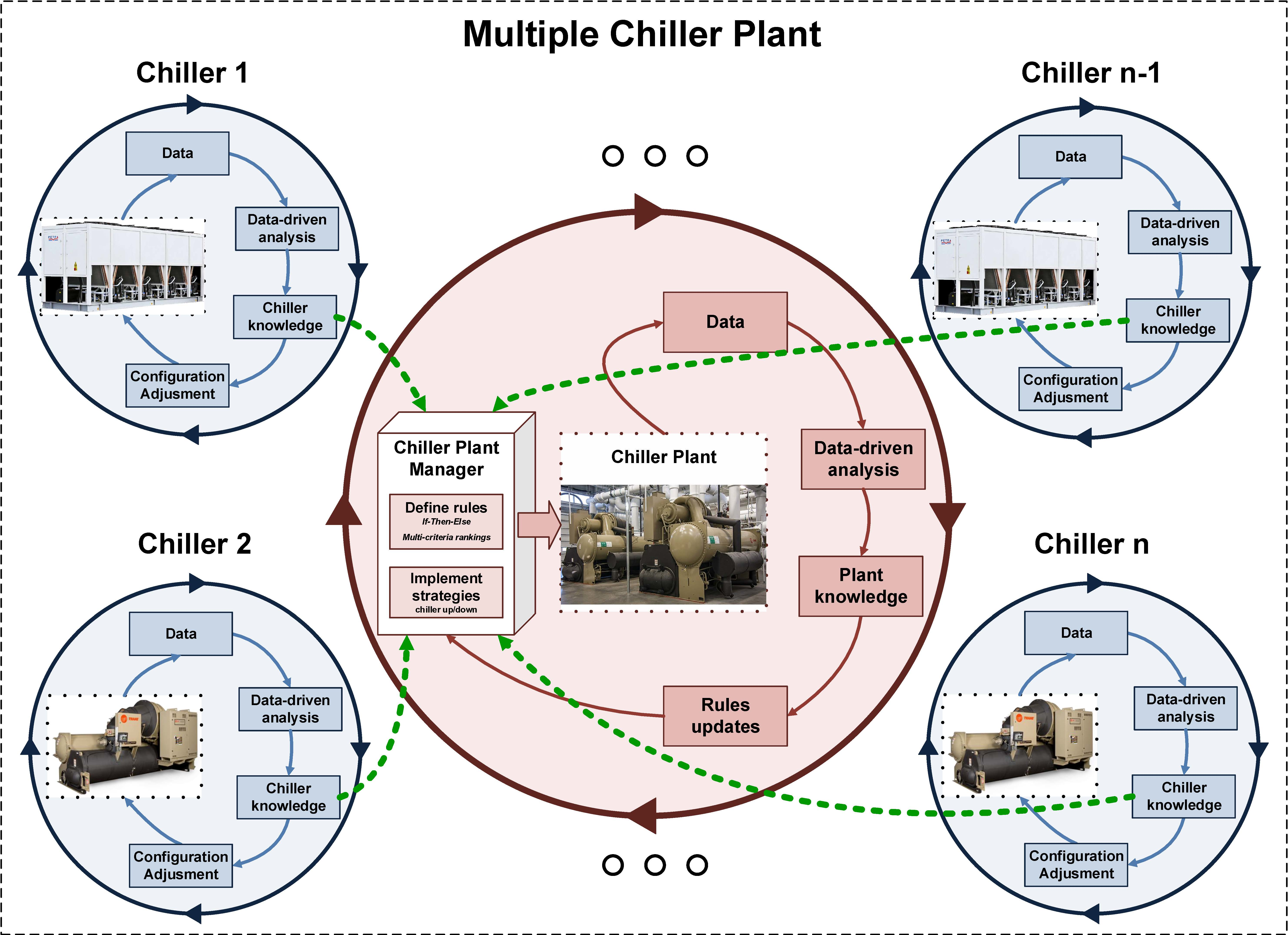
In this paper, we propose a data-driven approach to define, upgrade and tune the rules of a PMS and, in consequence, to improve energy efficiency in multiple-chiller plants (see Figure 1). The data analysis provides, on the one hand, information about individual chillers and, on the other hand, information about the chiller plant. The aim of chiller data analysis is to enhance individual chiller efficiency, whereas the objective of plant data analysis is to enhance overall plant efficiency. The knowledge about individual chiller performance is used for two purposes: to adjust internal chiller parameters and to define or tune rules implemented in the PMS. For that, conditional rules (If-Then-Else) allow us to decide when a chiller should be staged up/down, whereas sorting rules based on multi-criteria rankings allow us to choose which chiller should start/stop (the fittest one in each situation). Finally, the knowledge extracted from the plant lets us update management rules. Our approach is based on a hierarchical multilevel control system, requiring the implementation of the coordination level (an expert system with the management rules) and some configuration actions in the local units (chiller control boards).
The proposed approach requires several iterative analyses in order to achieve an optimal efficiency in the plant, but it has the advantage of low computational cost. For that reason, the application of the proposed approach can include new data from subsequent years, providing an incremental improvement in efficiency to the plant.
In a first step, we propose acquiring data from chillers and carry out an individual data-driven analysis. Using the extracted knowledge about chillers, internal chiller parameters are adjusted to improve their operation. Moreover, knowledge of each chiller is used to implement the management rules in the chiller PMS. Unlike complex optimization methods, heuristic rules can be implemented using simple programming structures and executed by any conventional building management system, without requiring extra computational resources.
In the second step, data from the whole plant are also collected and analyzed in order to obtain global knowledge about the plant. This step allows us to redefine and tune the rules or to add/delete sorting criteria regularly in the PMS.
Prior to their analysis, data must be collected from the BMS logs. Chiller-wise and overall plant COPs, which can be computed using chiller power and cooling load, are used as energy efficiency indicators. Data from other variables, such as chiller load ratio, condensing pressure and temperature, compressor current, outdoor temperature, etc., can also be considered for the analysis.
The data analysis of chillers and plant performance is based on highlighting relevant information by applying aggregation operations on measures, subject to some attributes [37]. Expression (1) represents, in a general way, those operations:
In our approach, average and counting samples are used as aggregation methods. Measures (the object of analysis) are energy efficiency indicators such as chiller and plant COPs, power demand and cooling load. Attributes are outdoor temperature, chiller load ratio, type of chiller, number of chillers running, year, month, day of year, weekday, hour, etc. Finally, data can be selected either from a specific chiller or from the plant. The attributes listed above can be also used to filter the data. For example, data from an specific weekday (Monday), hour interval (0–8 h), outdoor temperature limit (C), etc. Expression (2) summarizes some operations which can be carried out in different data analyses:
Data projections can be completed using visualization techniques to incorporate extra information [38]. For that purpose, additional attributes can be coded with properties such as size, texture, color, shape or weight, given a projection .
Other additional variables (condensing pressure and temperature, compressor current, etc.) can be also involved in the data analysis of each chiller. In this case, the addition of their information in terms of simple time-series plots can help us to monitor the chiller behavior.
From the knowledge acquired about each chiller performance, modifications in its internal configuration can be suggested. Note that local chiller control is implemented by manufacturers and they often only allow us to modify schedules and setpoints within a specific range. Parameters such as output water temperature, control zone, rate of changes, slide percentage, delays, etc. can be modified in order to improve chiller efficiency.
Data-driven analysis also provides information about how attributes influence the chiller and plant efficiencies. That knowledge is converted into management rules which are implemented in an expert module of the PMS. In this sense, the extracted knowledge is used to setup chillers, in order to update the set of conditional rules or to change their sorting criteria, resulting in appropriate plant management strategies. The staff in charge of energy management in the building should be involved in performing the data analyses and defining or tuning the management rules. They could provide their expertise and approve the management rules before their deployment on controllers.
The strategies to decide when chiller stages up/down can be implemented using basic programming structures, executable by any building management system (see Expression (3)):
Basic logic operations (AND , OR , NOT ), comparison operators () and math functions () can be used to define complex relationships among variables (see Expression (4)). Furthermore, nonlinearity strategies based on Fuzzy logic could be also applied using these conditional rules [39]:
These strategies constitute an expert module that determines the actions the PMS (Chiller up/down, up/down disable and no change) performs on the chiller in operation, according to the set of rules and sensor data in every situation. As an example, these management rules could be expressed according to Expression (5):
The strategies to select which chiller starts/stops are defined. They can be implemented using multi-criteria rankings. The criteria must be established beforehand: for example, total running hours, count starts, efficiencies, priorities, chiller loads, etc. can be used. For each criterion, a sorting order has to be chosen (ascending or descending order). The proposed procedure is to create one table for each criterion ”c” with n rows (as many as chillers) and two columns (the chiller index and the values of the corresponding criterion). Next, these tables are sorted, obtaining the chiller rankings for each criterion. Finally, a suitability table is obtained by weighting all previous rankings. According to all criteria, the most suitable chiller to start/stop among the available ones will be on the top of the table. All criteria can be weighted either equally (weights = 1/c) or differently (even excluding some criteria with zero weight, provided that the sum of all weights is 1). The following expression describes the sorting rules, based on multi-criteria ranking:
4. Description of the Chiller Plant at the Hospital of León
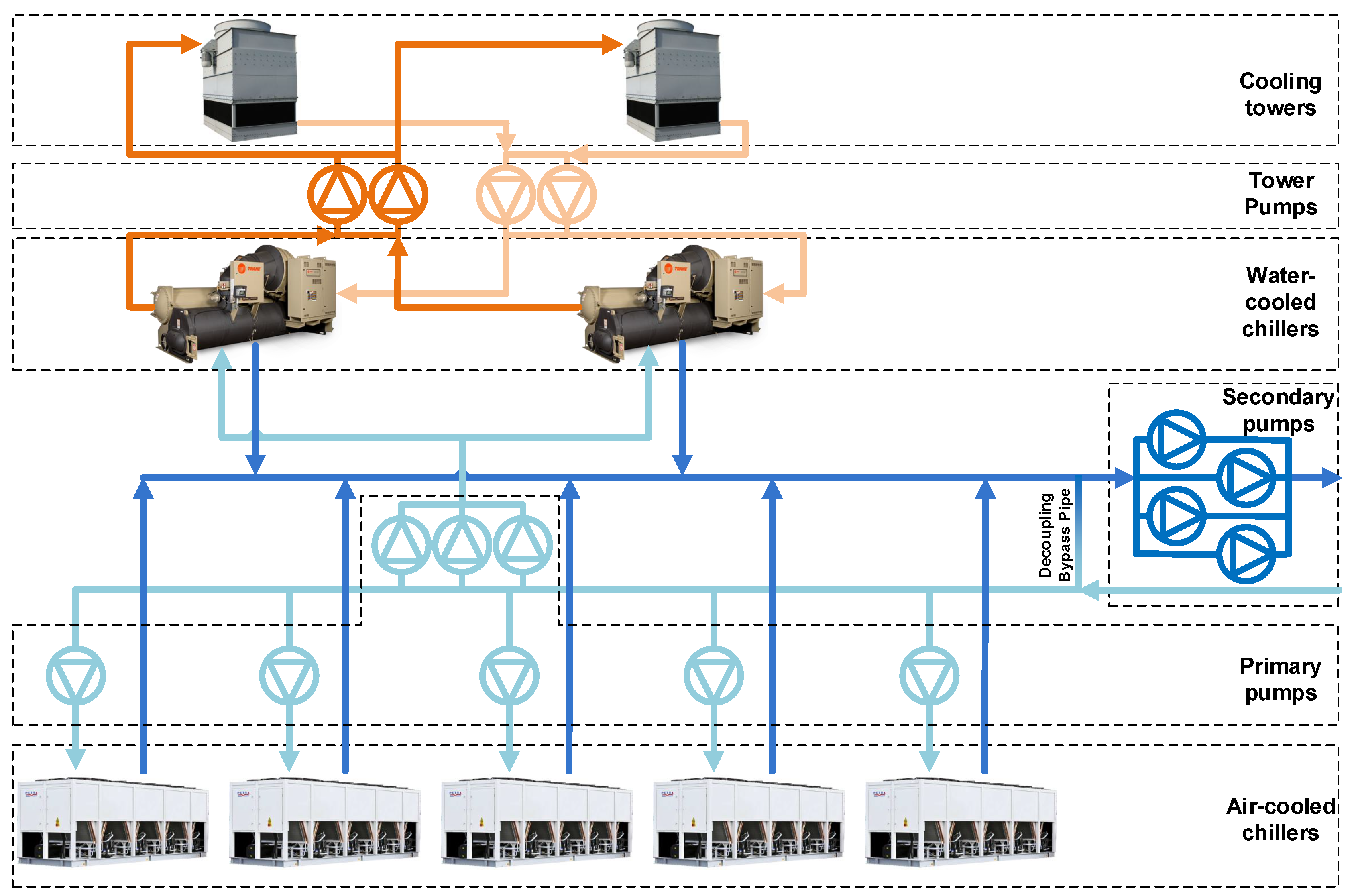
The chiller plant at the Hospital of León can be divided into a chilled water production system and a distribution system. In the production system, air-cooled and water-cooled chillers can be found. The distribution system comprises the decoupling bypass pipe and a variable chilled-water flow system. Figure 2 displays the general structure of the water flow system. Note that the colors of the streams try to represent the temperature of the water through the pipes during normal operation of the plant.
4.1. Production System
The main components of the chilled water production system at the Hospital of León are two groups of chillers: air-cooled and water-cooled chillers. Additionally, valves, sensors and pumps are needed to manage the chiller operation.
4.1.1. Air-Cooled Chillers
The plant comprises five identical air-cooled chillers. Each chiller needs a primary pump to force water flow through the evaporator and an on/off valve to avoid water flow when the chiller is not running.
- Chiller: The model is a Petra APSa 400-3, with a maximum cooling capacity of 400 tons (approximately 1407 KW). It includes three identical and independent refrigeration circuits (of 469 KW each one). Each one is composed of a screw compressor, an electronic expansion valve (EEV), and three individual condensers in V form. A common evaporator is used for the three circuits. The compressor has a maximum displacement of 791 m/h of R134a refrigeration gas, its capacity can be regulated between 50–100% of the maximum value by means of two auxiliary loading and unloading valves, and it is driven by a three-phase induction motor (400 V; 109 KW). The condensers use 16 fans of 1.5 KW, driven by ABB ACH550 variable speed drives. The control board is provided by Micro Control Systems. The nominal chiller COP is 4.3 (with Condensing temperature: 40 C; Evaporating temperature: 0 C).
- Primary pump: It is a Grundfos TDP 150-200/4 whose function is to maintain a water flow through the evaporator, depending on the cooling load. It is driven by a three-phase induction motor (400 V; 15 KW). A variable speed drive (Danfoss VLT HVAC FC 102), drives the pump, although the traditional star-delta starting is also available.
- On/Off valve: It is a Siemens Acvatix SQL33, installed on the return pipe to block water flow through the evaporator when the corresponding chiller is stopped.
- Sensors: Several sensors are installed on pipes, associated with the chillers. An on/off flow sensor is used to confirm whether chilled water flows or not (Siemens QVE1900). Moreover, a differential pressure sensor (Siemens QBE61.3-DP10) is connected to measure the flow. In addition, the temperature of output chilled water is measured (with a Siemens QAE2120.010).
4.1.2. Water-Cooled Chillers
The plant comprises two identical water-cooled chillers. Three primary pumps are used to force water flow through the evaporator, whereas an on/off valve cuts water flow when chiller is stopped. Furthermore, in this case, a cooling tower and tower pumps are required for condensing.
- Chiller: The model is a Trane CVGF650 with a maximum cooling capacity of 650 tons (approximately 2286 KW). It comprises only one refrigeration circuit with a centrifugal compressor, an electronic expansion valve (EEV) and tubular heat exchangers (for evaporator and condenser). The compressor works using R134a refrigeration gas and its capacity can be regulated between 50–100% of the maximum value, by changing the angle of turbine blades. It is driven by a three-phase induction motor (400 V; 367 KW). The nominal chiller COP is 6.23 (Condensing temperature: 40 C; Evaporating temperature: 0 C).
- Primary pumps: There are three Grundfos NK 125-250/247/A/BAQE pumps that are started, depending on the cooling load, in order to maintain a water flow through the evaporator. They are driven by a three-phase induction motors (400 V; 18.5 KW), with star-delta starting.
- On/Off valve 1: It is a Bernard OA15, installed on the return pipe to block water flow through the evaporator when corresponding chiller is stopped.
- Cooling tower: The Baltimore Aircoil Company S-3654-NM cooling tower enables the control of condensing temperature, transferring heat to the environment when condensing water evaporates. An axial fan, driven by a three-phase induction motor (400 V; 18.5 KW) and managed by a variable speed drive (Moeller DF6-340-22K), helps the heat exchange. Moreover, it incorporates three resistors of 5 KW to avoid water freezing.
- Tower pumps: There are two groups of two Grundfos NK 150-315/307/BAQE pumps each, one to propel condensing water to the cooling tower and the other to maintain a water flow through the condenser. They are driven by three-phase induction motors (400 V; 30 KW), with star-delta starting.
- On/Off valve 2: A Bernard AS25, which allows for selecting which cooling tower will be used for condensing.
- Sensors: Several sensors are installed on pipes, associated with the chillers. An on/off flow sensor is used to confirm whether chilled and condensing water flows or not (Johnson Controls F61SB-9100). In addition, the temperatures of input and output chilled water are measured (Johnson Controls TS-9101-8224).
Table 1 summarizes the nominal chiller data in the plant at the Hospital of León.
4.2. Distribution System
The design of the distribution system enables variation of chilled water flow using a set of four secondary pumps (Grundfos NK 125-400/375/BAQE) driven by four three-phase induction motors (400 V; 55 kW) with their corresponding variable speed drives (Danfoss VLT 6000 HVAC and Schneider Electric Altivar 61). The aim of this system is to adjust the building load to the instantaneous cooling demand. In addition, pressure variations due to differences between cooling generation and consumption are alleviated by the decoupler piping placed between supply and return pipes. Additionally, a cooling meter and supply/return temperature sensors allow us to measure demanded cooling energy.
5. Application of the Proposed Approach to a Chiller Plant
The proposed methodology has been applied to the multiple-chiller plant at the Hospital of León. As mentioned above, that plant comprises two different chiller groups: five air-cooled chillers (ACC1–ACC5) and two larger water-cooled chillers (WCC1, WCC2). The first aim of our approach is to analyze the operation of chillers in order to acquire knowledge (detect failures or malfunctions, extract patterns, find external influences, etc.). The final aim is to analyze the operation of the plant in order to monitor its efficiency and tune or upgrade control rules, if necessary. Thus, our approach requires past data of the chiller and plant to carry out the analyses. For that reason, data were collected from the BMS, including variables, such as COP, cooling load, power demand, chiller load ratio, condensing pressure and temperature, compressor current, outdoor temperature, etc. Data were gathered every 1 min during a one-year period, so 525,600 samples were obtained for each variable. The chiller plant is located in León, a city with continental climate where cooling loads have a clear seasonal nature. Therefore, data from a whole year should cover that seasonal behavior. Nevertheless, the addition of more data in subsequent years would improve the coverage.
5.1. Data-Driven Analyses and Knowledge about the Chillers
Using data from chillers, an analysis was carried out for each one, focusing on the chiller behavior and its operation with regard to external conditions such as chiller load ratio or outdoor temperature.
Prior to the study, maintenance staff inspected the main chiller control and protection elements (valves, solenoids, relays, sensors, fuses, etc.), with the aim of repairing them, if required. Faults in control relays, broken fuses, damaged solenoids, blocked valves, earth defects or wrong wirings can provoke abnormal chiller operation. Once faults in chiller elements are detected and corrected, the analyses were performed. In this case, time series plots were used for checking the R134a refrigeration cycle with its main parameters (gas suction, discharge temperature and pressure). Sharp oscillations were discovered in the control signal acting on condensing fans of ACC1. The condensing pressure was higher than normal, being affected by those variations. Thus, this high pressure caused electricity peak demands, adversely affecting the chiller efficiency Moreover, it provoked damages on air-cooled chiller elements—for example, the solenoid of some loading and unloading valves broke down frequently, fan bearings suffered strong strains, compressors were working in extreme conditions affecting the compression ratio, etc. The remaining air-cooled chillers showed similar behavior, so condensing control setpoints were verified in order to reduce condensing pressure (below 900 KPa) and smooth the control signal. Variables involved in the R134a refrigeration cycle of water-cooled chillers were in a normal range.
First of all, chiller operation at partial loads was analyzed. Studying the chiller performance at partial loads is very important since rarely chillers run at their nominal load (only a few hours per day). Air-cooled chillers can modulate cooling capacity between 0.22 and 1.0 of nominal value, whereas water-cooled chillers can regulate capacity from 0.5 to 1.0. It should be remarked that the nominal capacity of water-cooled chillers is 1.6 times higher than that of the air-cooled chillers (2286 KW versus 1407 KW). Some aggregation operations are applied to each chiller data set according to the following expression:
Figure 3 shows the relationship between COP and chiller load for two kinds of chillers (ACC1 and WCC2). In Figure 3a, it can be observed that ACC1 COP remains constant with regard to the load (around 3.7). However, WCC2 COP has an exponential relationship with load, with a maximum value of 5.2 and a minimum value of 2.5, when the chiller runs at the half capacity (see Figure 3b). Therefore, water-cooled chillers operation should be avoided when the cooling load is lower than 1143 KW for a long time. In this case, air-cooled chillers with a better load partition are preferable, since their capacity can be regulated up to 310 KW, keeping a constant performance.
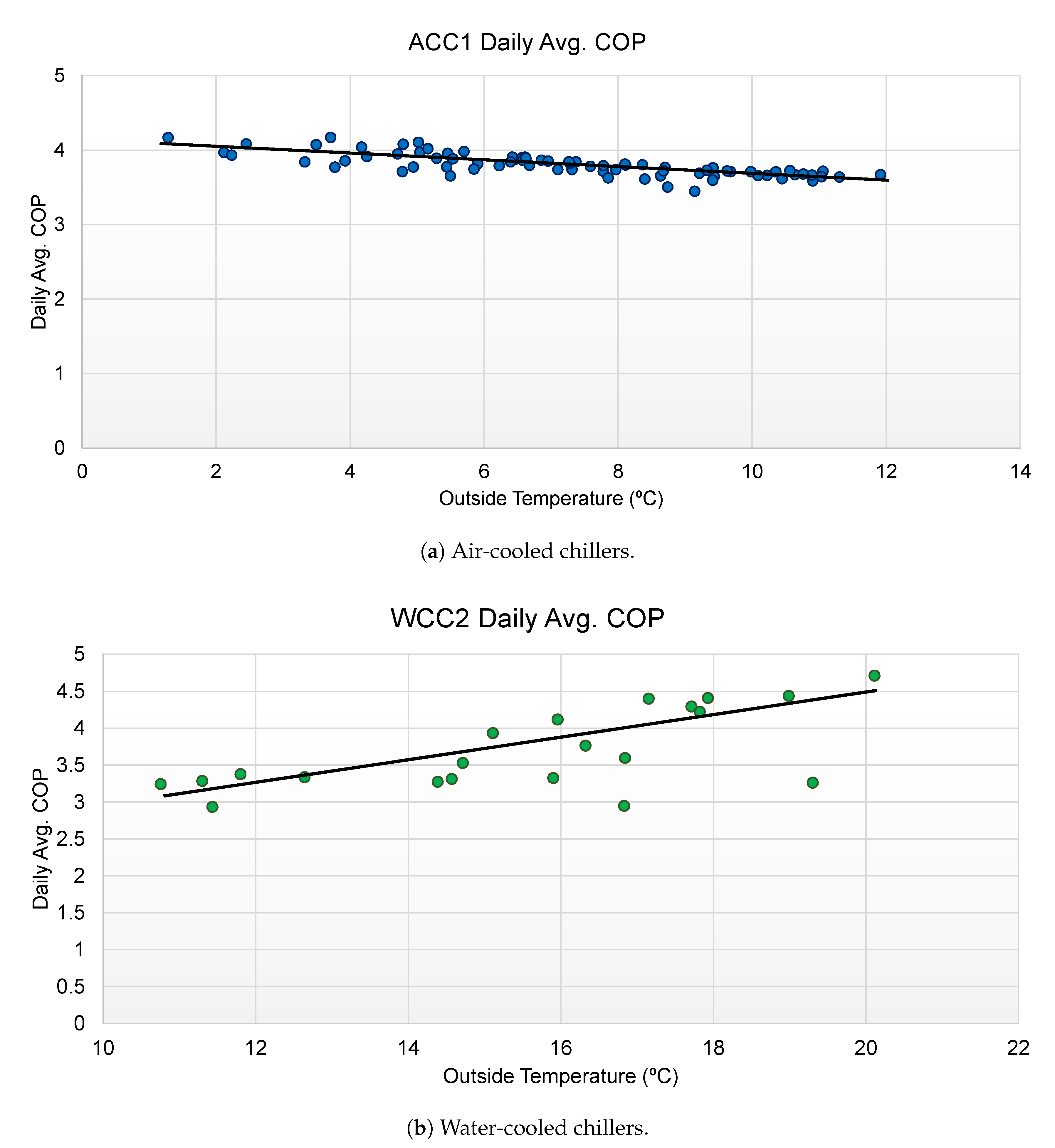
Next, the chiller operation regarding to outdoor temperature is analyzed. For that purpose, aggregation operations are applied to each chiller data set according to the following expression:
As can be seen in Figure 4, outdoor temperature influences negatively the air-cooled chiller performance, whereas COP for water-cooled chillers increases with outdoor temperature. Observing Figure 4a, ACC1 COP decreases slightly when temperature increases, since the heat exchange with air becomes difficult. However, daily average COP is always greater than 3. Looking at Figure 4b, it can be pointed out that daily average COP can reach high values, greater than 3. Nevertheless, lower COP values can be achieved when outdoor temperature is below 12 C. This is due to water-cooled chillers run at a low load ratio with low cooling loads. Thus, air-cooled chillers should run those days when average temperature is below 12 C. Water-cooled chillers should run on days with an average temperature above 16 C. In the range 12–16 C, all chillers can operate and other patterns should be considered.
Summarizing what was learned about the chillers, it can be stated that air-cooled chillers should be started with low outdoor temperatures, when cooling load is low. On the other hand, water-cooled chillers should be run with high cooling loads, ensuring that the chiller load ratio is quite high. Condensing control, especially on air-cooled chillers, should be adjusted since high condensing pressures and strong oscillations have been detected.
After the chiller analyses, it can be necessary to adjust the internal configuration of chillers. The maintenance staff was advised to adjust some parameters, especially the configuration of air-cooled chillers. The main changes in the internal configuration of the chillers were focused on slightly increasing the deadband in temperature control, improving the chiller response in the presence of short peak cooling loads, minimizing the operation cycles of capacity control valves, reducing the proportional action in condensing control, balancing refrigeration circuits and avoiding unsafe compressor runnings. Note that manufacturers do not allow us to modify remotely some internal parameters and they are only accessible through the local panel with the right access privileges. Table 2 summarizes the parameters modified in air-cooled chillers after chiller analyses.
The configuration of water-cooled chillers was also examined, but, in this case, most of the internal parameters remained unchanged. Just a few parameters were adjusted to be in coherence with the water flow system. As in air-cooled chillers, the temperature setpoint was also decreased due to the unbalance of primary and secondary chilled water flows. It causes a recirculation excess of return chilled water through the decoupling bypass pipe.
5.2. Converting Knowledge into Management Strategies
Once knowledge about the chillers was extracted and operators upgraded the internal configuration of each one, our efforts focused on designing and implementing efficient chiller management strategies, which can be incorporated into a PMS. Note that chiller operation is automated and data are stored by BMS.
5.2.1. Architecture of the Plant Manager Software
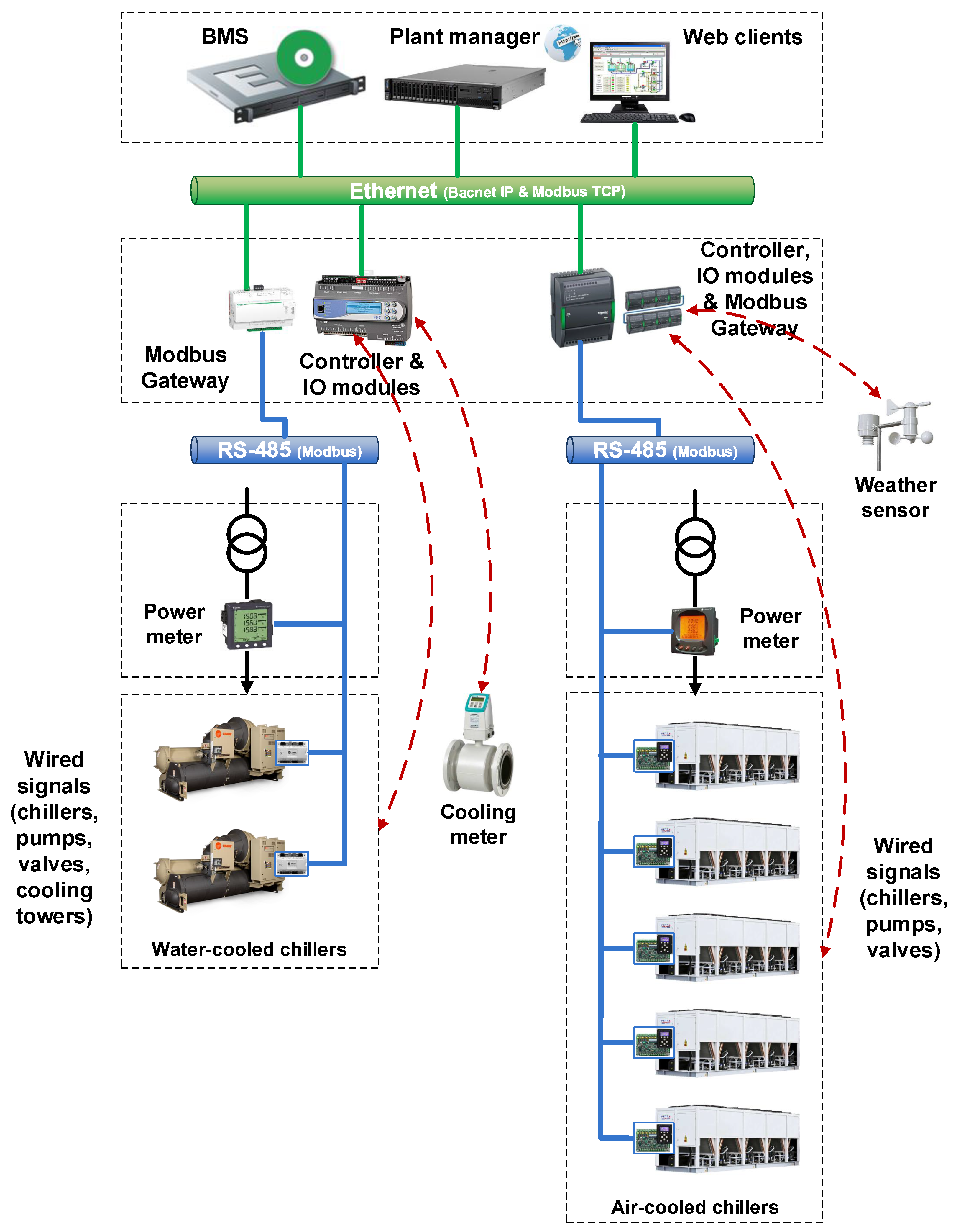
An automatic existing system was modified for chiller plant management at the Hospital of León (see Figure 5). The system is based on an ad hoc software which implements management strategies. The PMS has been developed as a Software as a Service (SaaS) application, so that web clients can easily access a software manager using a standard web browser to manage the chiller plant.
The BMS communicates with two controllers (one for air-cooled chillers and the other for water-cooled chillers) using the BACnet IP protocol. The BMS receives all signals from both controllers (chillers, valves, pumps, cooling towers, etc.) for monitoring purposes and sends them start/stop commands and setpoints. The PMS decides which chiller should be staged up/down and when, and communicates with BMS using also BACnet IP.
The first controller (AS by Schneider Electric) is used to implement control of air-cooled chillers and auxiliary elements (valves, primary pumps, etc.). Additional I/O modules capture signals from field elements and weather sensors. This device also works as a Modbus gateway to communicate with chiller cards and retrieve internal variables. The AS controller stores data in local logs and gradually transfers them to the BMS. The second controller (FEC by Johnson Controls), with integrated I/O modules, is used to implement control of water-cooled chillers and their auxiliary elements (valves, primary pumps, tower pump, cooling tower, fan, etc.) and to read building cooling meter. The FEC controller stores data in local log files and gradually transfers them to BMS too. Additionally, a protocol interface card (Trane PIC BAS-SVX08D-E4) has been installed in each water-cooled chiller to gain access to their internal variables and parameters. This card provides data using Modbus RTU protocol. A gateway (Com’X 510 by Schneider Electric) is necessary to convert Modbus RTU to Modbus TCP. On the other hand, power meters measure the main variables of electricity supply to both groups of chillers. They are also connected to Modbus RTU networks to communicate with BMS.
5.2.2. Defining Rules
Using knowledge about the chillers, several sets of rules are defined, tuned or upgraded. These rules are the core of an expert module that uses them to manage the plant efficiently. The following aspects are taken into account in the rule definition:
- Reliability and security of supply of chilled water (since a hospital has critical systems such as the refrigeration of surgeries, magnetic resonance systems, scanners, a data center, HVAC systems in patient rooms, etc.).
- Maximization of the plant operation by choosing the most efficient chiller (or combination of chillers) available to meet the required cooling load.
- Maximization the chiller efficiency by enforcing high chiller loads.
- Reduced maintenance of the chiller plant (the manager should balance running time and start counts for all chillers).
- Adjustment of the plant operation according to weather conditions (mainly, outdoor temperature).
- Automatic and manual operation modes of the chiller plant. The manager should consider user preferences, either giving priority to a chiller or enabling/disabling an specific chiller.
The basis of sequencing method is the measurement of the cooling load and the computation of the current operating capacity, based on all chiller load ratios. If cooling load is greater than chiller capacity during a short period of time, a new chiller will be started. Otherwise, a running chiller will be stopped. Prior to proceeding, it is checked that the chiller load is decreasing. Note that the plant requires, at least, one chiller running in order to provide the base cooling load to the building. In other cases, a schedule could be considered to stage up/down chillers. A chiller will be also stopped when consecutive running time exceeds the rotation setpoint (168 h). Additional rules considering supply and return chilled water temperatures are also defined in order to ensure cooling supply to the building. These rules contain extreme thresholds and will be activated in exceptional situations, keeping chilled water temperature in range [6–10] C. Note that simple rules can be combined using logic operations in order to build advanced rules. Table 3 summarizes the main rules used to stage up/down chillers.
Some rules taking into consideration the physical environment are defined. The plant contains different types of chillers and their efficiencies are influenced by external conditions as data analysis revealed. Therefore, it is required to decide which type of chiller should be running in each situation. In this way, outdoor temperature is used for creating such delimiting rules. Average temperature is computed each day and used to predict the conditions of the following day. If daily average outdoor temperature of the previous day was higher than 16 C, then the chiller selected to stage up/down will be a water-cooled chiller (WCCy; y = 1–2). If daily average outdoor temperature of the day before is lower than 12 C, then the chiller selected to stage up/down will be an air-cooled chiller (ACCx; x = 1–5). In the range [12–16] C, other rules will be taken into account. An overview of delimiting rules can be seen in Table 4.
Exclusion rules are required in order to determine when to disable chiller up/down commands due to either alarms or planned maintenance tasks. User can enable/disable a chiller from the web interface. On the other hand, if power demand exceeds 1300 KW in the plant, a new chiller starting is blocked and a warning is triggered (a user check is required to allow staging up a new chiller). That avoids peak power demands and inefficiencies in the plant provoked by anomalous operations. Moreover, stopping a chiller is disabled as long as the idle capacity is less than the load ratio of the chiller to stop. An overview of exclusion rules can be seen in Table 5.
Finally, rules for sorting chillers are defined with the aim of determining which chiller starts/stops. First, different criteria are established and, later, the corresponding chiller rankings are obtained. Table 6 summarizes the sorting rules.
In the stage up sequence, criteria such as chiller priorities, efficiencies, total running hours, hours from last stop and start counts are used. A weighting method is applied, balancing all criteria and obtaining a weighted ranking. The chiller on the top of that ranking should have a high position in the partial rankings, matching most of the criteria. For example, the next chiller to start should have a high priority, noteworthy efficiency, lower total running hours and start counts and it should not have been stopped recently, i.e., the chiller should have a high position in all rankings. In this case, the same weight is applied for each criterion. However, different values could be used:
In the same way, the criteria for the staging down sequence are relative running hours, chiller loads and efficiencies, which are weighted to decide the chiller to stop. Note that sorting chillers according to the COP is now performed in the opposite order. For instance, the next chiller to stop should have the lowest efficiency and load ratio and should also have been running for many consecutive hours:
5.2.3. Plant Management Strategies
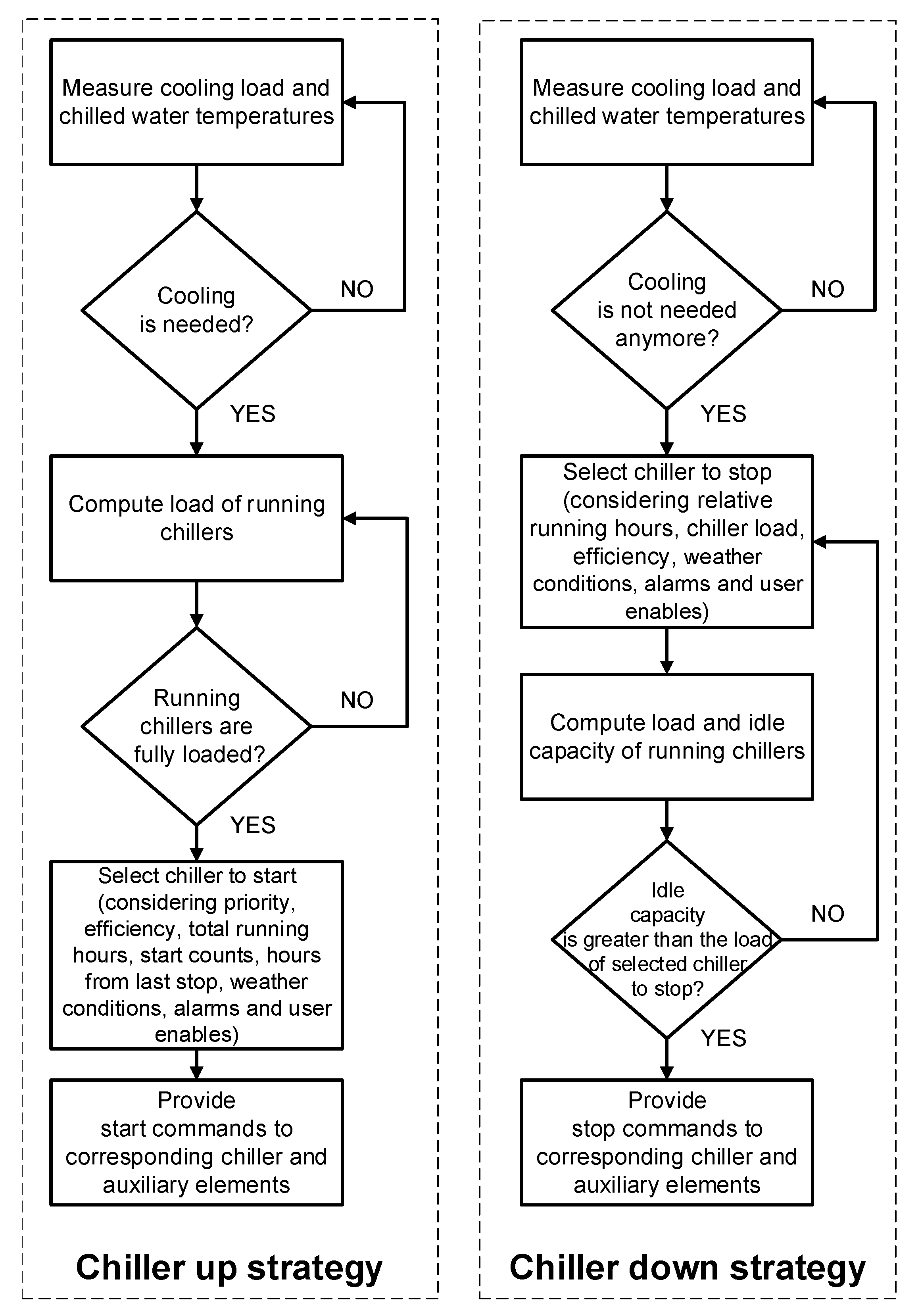
Using the previous sets of rules, efficient management strategies are implemented on the ad hoc software. Mainly, two strategies determine chiller sequencing: “chiller up” and “chiller down” (see Figure 6). The “chiller up” strategy monitors the cooling load (measured by a cooling meter) as well as the supply and return chilled-water temperatures. If the cooling demand increases and the running chillers are fully loaded, a new chiller is started. Depending on supply and return chilled water temperatures, the chiller is started immediately or after a short delay (trying to absorb transitory load fluctuations). The criteria described in the previous section are applied in order to decide which chiller starts. Furthermore, it is checked the presence of alarms (such as the internal faults in chillers and auxiliary elements) and the user activations (a chiller can be disabled due to maintenance tasks). The prediction of the outdoor temperature is also considered in order to take advantage of weather conditions. Finally, the manager sends commands up to BMS and it provides start commands to the selected chiller and its auxiliary elements, such as valves, pumps, etc., and verifies possible alarms in the starting sequence.
The “chiller down” strategy also monitors the cooling load and supply/return chilled water temperatures. If the manager detects that cooling is not needed anymore (because of a decrease in cooling load and a sudden drop in chilled water temperature), one of the running chillers should be stopped. The criteria described in the previous section are applied in order to decide which chiller stops. Before making that decision, the software must verify that the remaining running chillers can absorb the cooling load of the chosen chiller. For that purpose, the manager computes the difference between the idle capacity of running chillers and the load of the chiller that is stopped. Finally, if idle capacity is slightly greater than the chiller load, the manager sends down a command to BMS and it provides stop commands in sequence to the selected chiller and its auxiliary elements.
These management strategies based on rules are used by the system in automatic mode (default). However, the system can be managed in manual mode, according to the staff expertise. The staff can vary setpoints, delays, thresholds and chiller activations.
5.3. Data-Driven Analysis and Knowledge about the Plant
Once the management strategies are deployed in the plant and new data are collected, an analysis has to be carried out to monitor plant efficiency. That study focuses on the plant operation and efficiency with regard to cooling load, external conditions, chiller sequencing, etc.
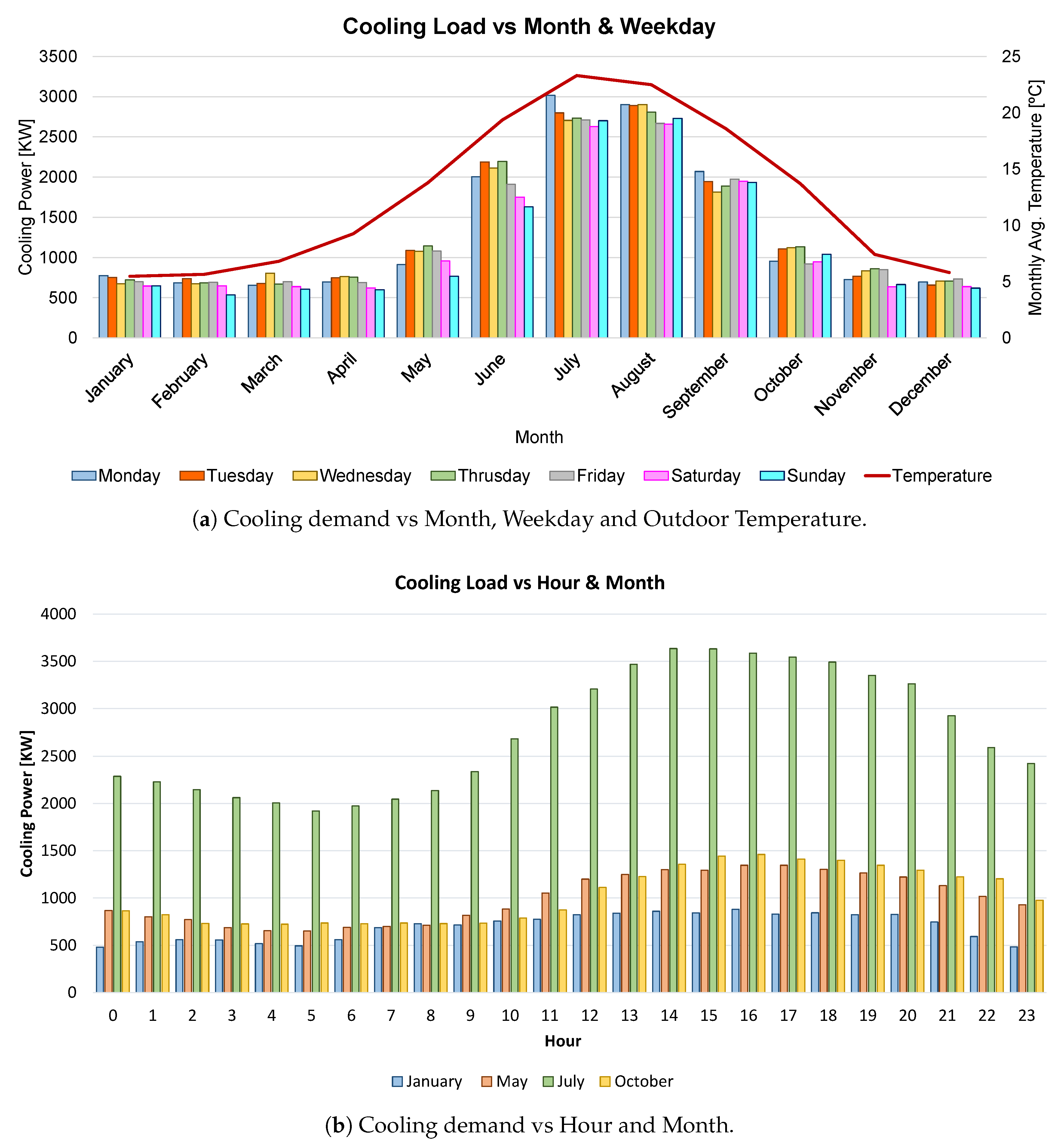
First of all, cooling demand is analyzed (see Figure 7) applying the following expression:
Figure 7a shows the average cooling load for each month and weekday. It can be seen that cooling demand has a seasonal evolution, exceeding 2000 KW in Summer and not exceeding 1000 KW in Winter. Therefore, water-cooled chillers should be run in Summer to cover the cooling demand. On the contrary, they could operate in Winter, but at half capacity, achieving lower COP. Due to lower nominal power and better load partition, air-cooled chillers are more efficient in that season. In Figure 7a, the average outdoor temperature is also represented. It can be seen that outdoor temperature influences directly on cooling load due to demand of HVAC systems. In May and October, free-cooling operation in those systems can be observed since cooling load does not follow the temperature evolution.
Figure 7b displays the average cooling load for each hour of the day and months. Only four representative months (January, May, July and October) have been represented only for simplicity. In winter (January), cooling load is quite flat during all the day, whereas, in Summer (July), it is flat at nights, becoming steep from 10 h on and decreasing after 22 h. In May (Spring) and October (Autumn), the day profile of cooling load is quite similar.
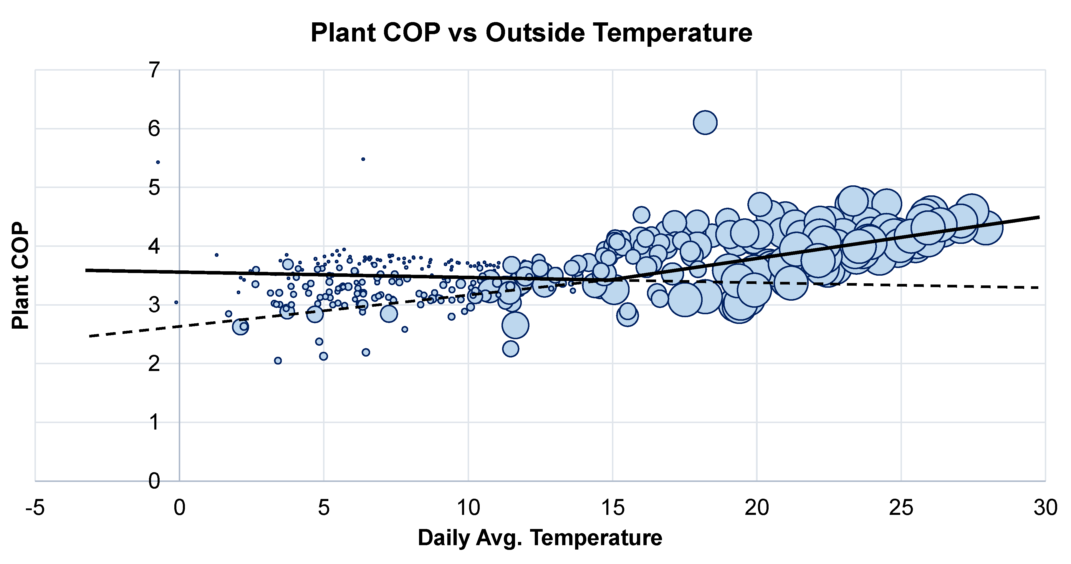
Next, the influence of outdoor temperature on plant COP is analyzed using the expression:
The daily average COP value was plotted with respect to the daily average temperature (see Figure 8). Note that the size of points represents the type and the number of chillers running: the smallest points correspond to one air-cooled chiller and the largest ones are from two water-cooled chillers. Three zones can be distinguished in the graph (below 10 C, above 20 C and between 10 C and 20 C). Lower temperatures imply low cooling loads (little use of HVAC systems), so air-cooled chillers (smaller points) are more appropriate, since condensing refrigerant using cold air is quite efficient. In contrast, higher temperatures entail high cooling loads (strong use of HVAC systems) and, therefore, water-cooled chillers (larger points) are more convenient because they have better performance and higher nominal capacity (so a smaller number of chillers is required to cover high cooling loads). It can be also seen that the plant COP would slightly decrease if air-cooled chillers run with temperatures above 20C. Similar results (plant COP reduction) would be obtained if water-cooled chillers run with temperatures below 10 C. Between 10 C and 20 C, some chiller combinations can be observed, depending on other factors considered by the management strategies.
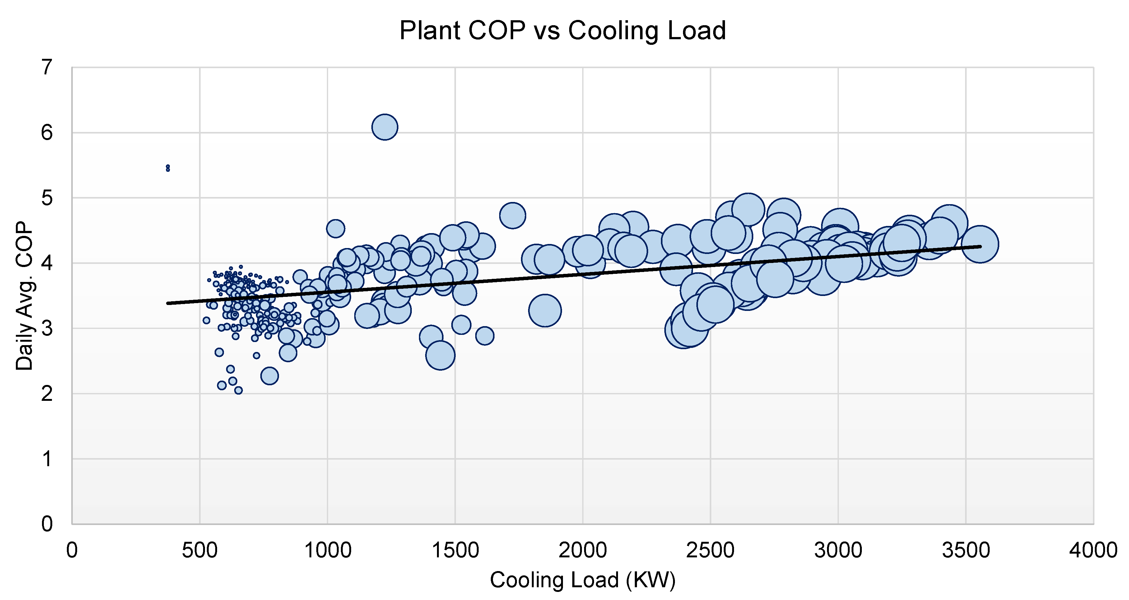
Analyzing the plant performance with regard to the cooling load allows us to verify the chiller sequencing management strategies. In this sense, the daily average COP was plotted with respect to the cooling load of the building (see Figure 9). The used aggregation was:
As in the previous figure, the size of points represents the type and the number of chillers running. It can be seen that, the higher the cooling load is, the better the plant performance is. High cooling loads are typically covered by two water-cooled chillers, with better individual performance. On the contrary, low cooling loads are provided by one air-cooled chiller, with finer load partition. Medium cooling loads can be covered by several chiller combinations (two air-cooled chillers, one water-cooled chiller or one of each).
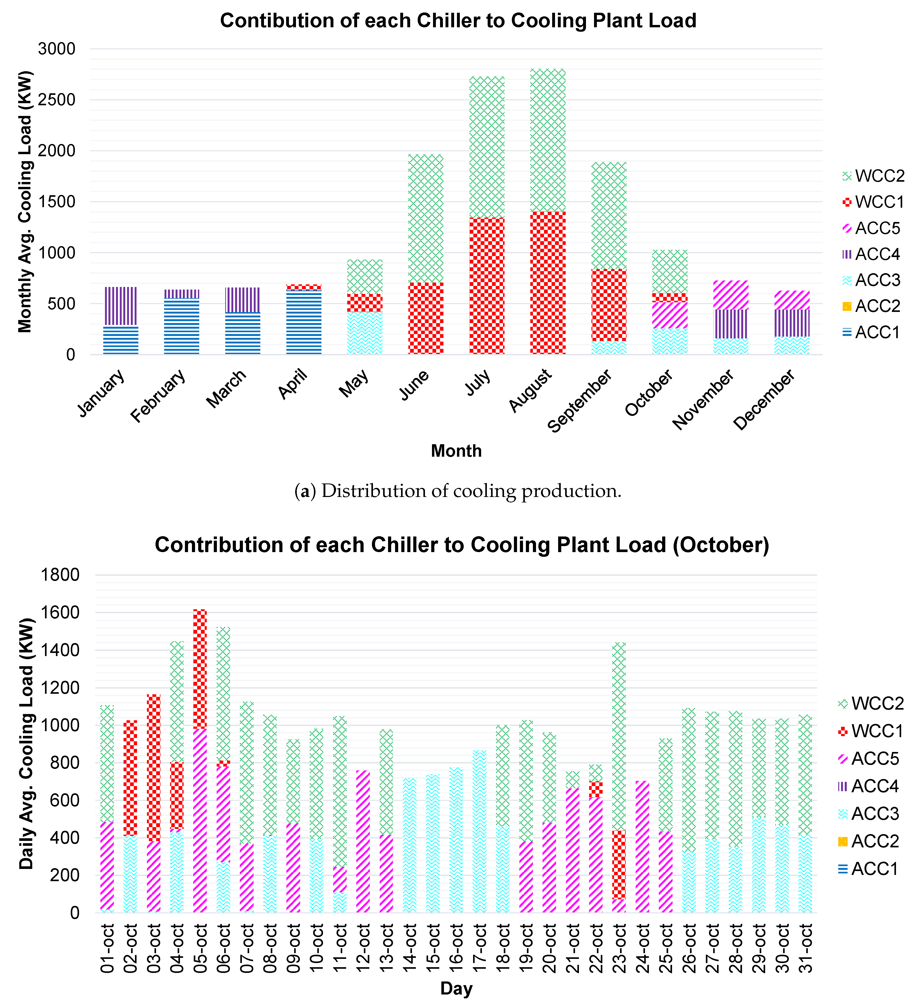
Studying the contribution of each chiller to the total cooling load of the building can also help us to verify the efficacy of chiller sequencing strategies (see Figure 10). The manager tries to consider external conditions and to balance several criteria (total running hours, start counts, priorities, efficiencies, etc.), choosing the fittest ones in order to cover the cooling load. It can be seen in Figure 10a that chiller sequencing has a seasonal behavior (as cooling load). In winter, cooling is provided by air-cooled chillers, whereas, in summer, cooling is generated by water-cooled chillers. During both periods, cooling is quite stable, so chillers only alternate their operation when the relative running hours exceed the rotation setpoint. For example, only ACC1 and ACC4 were running in January, and only WCC1 and WCC2 produced cooling in August. In spring and autumn, the manager combines the operation of air-cooled and water-cooled chillers, since cooling varies daily. Therefore, the manager has to send up/down commands daily to the chillers in order to cover fluctuating cooling load. Focusing on October (see Figure 10b), it can be confirmed that up to three chillers were started during a day (October 6th). This causes the rise of start counts, a crucial step in the sequencing, and thus an increasing possibility of appearing faults.
Summarizing the knowledge about the plant, it can be observed that cooling load at the Hospital of León has a noticeable seasonal and daily behavior, so a different operation can be established each season. Outdoor temperature can be used to predict abnormal days with regard to the current season. Two hours (10 h and 22 h) of daily profile can be used as indicators of the expected cooling load (hours in which the cooling load usually increases or decreases, respectively). In order to avoid the increase of start counts in spring and autumn, chiller down command can be delayed until the idle capacity is a bit higher.
Updating Rules
Rules set can be updated in three ways:
- Tuning the threshold. The original rule is maintained, but the threshold which triggers this rule is modified. For example, as long as the capacity of running chillers does not drop below 0.6 (not 0.7), a running chiller will not be stopped, avoiding the increase in the number of start counts.
- Upgrading the complete condition. The rule is redefined completely, either establishing new premises or combining individual ones. For instance, outdoor temperature allows us to adapt the seasonal and daily operation. Furthermore, cooling load at certain hours allows us to estimate its evolution.
- Tuning criteria and weights. Sorting rules can be changed either by adding/deleting a criterion or adjusting the weights. Staff can vary weights from the web interface, for instance, to consider only one criterion (its weight is 1 and the remaining ones are 0) or to weight some criteria more than others (being the sum of weights 1). However, during this work, criteria have not been modified.
An overview of updated rules can be observed in Table 7.
6. Results and Discussion
After the application of the proposed approach, some efficiency enhancements have been obtained in the multiple-chiller plant at the Hospital of León. Below, these results for the individual chillers (ACC1–5, WCC1–2) and overall plant are presented. For that purpose, COPs corresponding to one year after changes were collected in order to compare them with the previous COPs before changes. Note that annual average outdoor temperature was very similar in both periods (11.2 C versus 11 C). Data acquired using a sampling time of one minute during a one-year period, i.e., 1,052,640 samples, are used in the projections.
6.1. Chiller Efficiencies
First, results on individual chiller efficiency are presented and discussed. Efficiency was monitored for each chiller according to the following expression:
The study focuses on ACC1 and WCC2 chillers, since they were running the greatest number of hours in that period.
Figure 11 shows the histograms of ACC1 and WCC2 COP corresponding to before and after chiller modifications. At a glance, it can be seen that COP indicator was increased for both chillers. For ACC1 (see Figure 11a), the average COP was increased from 3.18 to 3.76, resulting a noteworthy enhancement of 18.35%. Mainly, it was possible due to two reasons. On the one hand, changes on condensing control setpoints caused the reduction of condensing pressure (200 KPa approx.) and, as a result, the power demand decreased. On the other hand, changes on condensing control parameters (mainly proportional action) ensured a more stable operation of air-cooled chillers. In case of WCC2 (see Figure 11b), the average COP was increased from 4.08 to 4.13, resulting in a slight enhancement of 1.22%. It was probably due to the adjustment of the chilled water setpoint and the reparation of cooling towers.
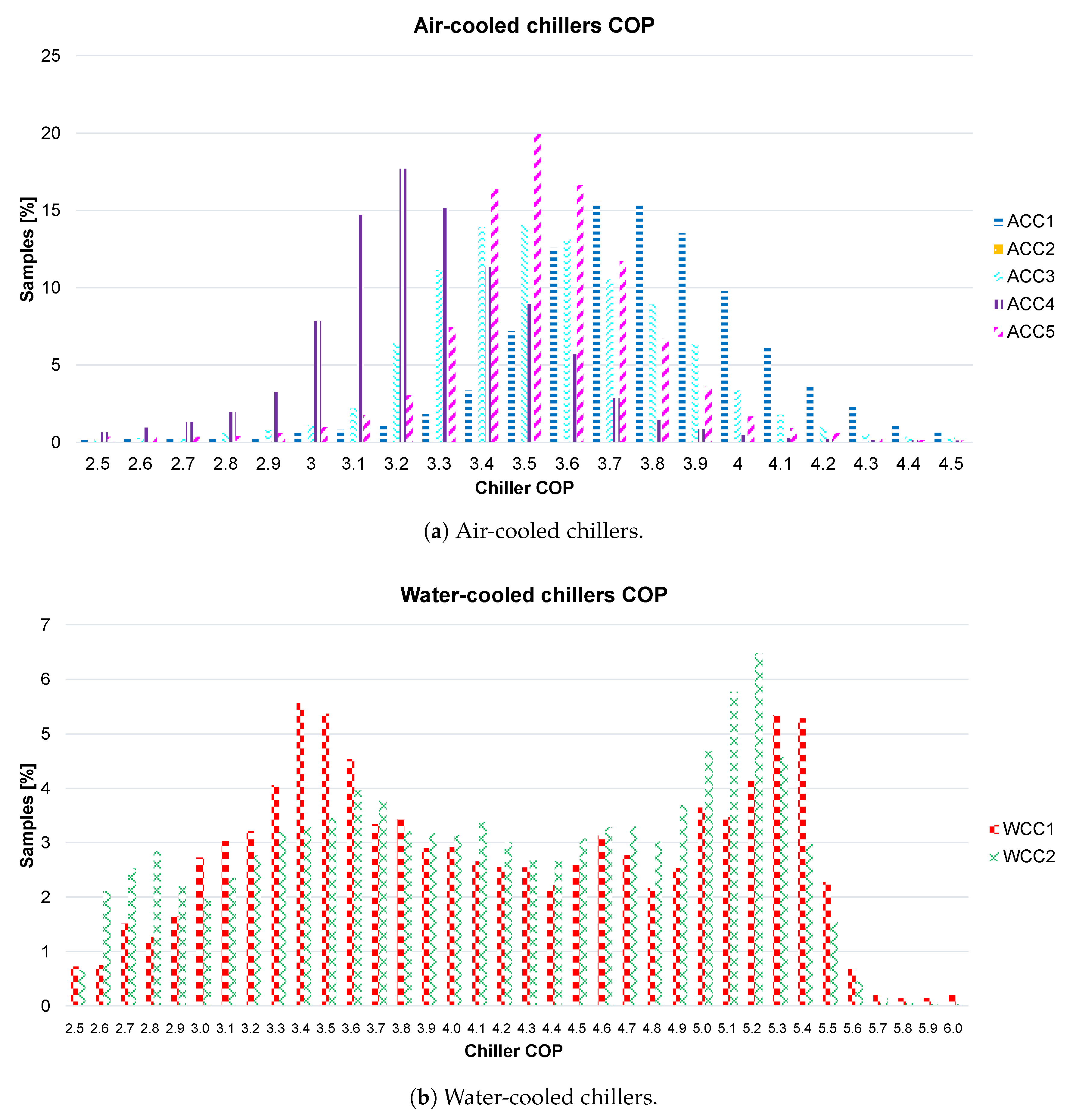
COPs of identical chillers have been compared with each other (see Figure 12) in order to detect deviations and inefficient operations. COP histograms corresponding to five air-cooled chillers (ACC1–5) are represented on Figure 12a. This comparison reveals a clear difference between ACC1 and ACC4 performance. At a glance, it can be observed that the COP of ACC4 is lower than the one of ACC1 (the histogram moved to the left), whereas the COP of ACC3 and ACC5 are located in the middle and they have a very similar performance. The noticeable difference between ACC1 and ACC4 performance could be due to the experiments carried out in order to test a new decoupled condensing control strategy in ACC4. Refrigerant charge was also checked, verifying that, for example, the pressure of R134a in ACC3 was lower than the nominal value. Furthermore, oscillating chiller operation could have affected the compressor ratio and the efficiency of other chiller elements, such as condensing fans. In fact, some fans have been replaced in ACC1. Regarding water-cooled chillers (see Figure 12b), no significant difference can be appreciated (apart from WCC2 run longer than WCC1), so both chillers have a similar efficiency indicator.
Table 8 summarizes efficiency results for all chillers. Note that high efficiency enhancements have been obtained for air-cooled chillers compared with water-cooled chillers. ACC2 was not running during the studied period due to severe electrical faults.
6.2. Plant Efficiency
The results on chiller plant efficiency are presented and discussed. Efficiency was monitored for overall plant according to the following expressions:
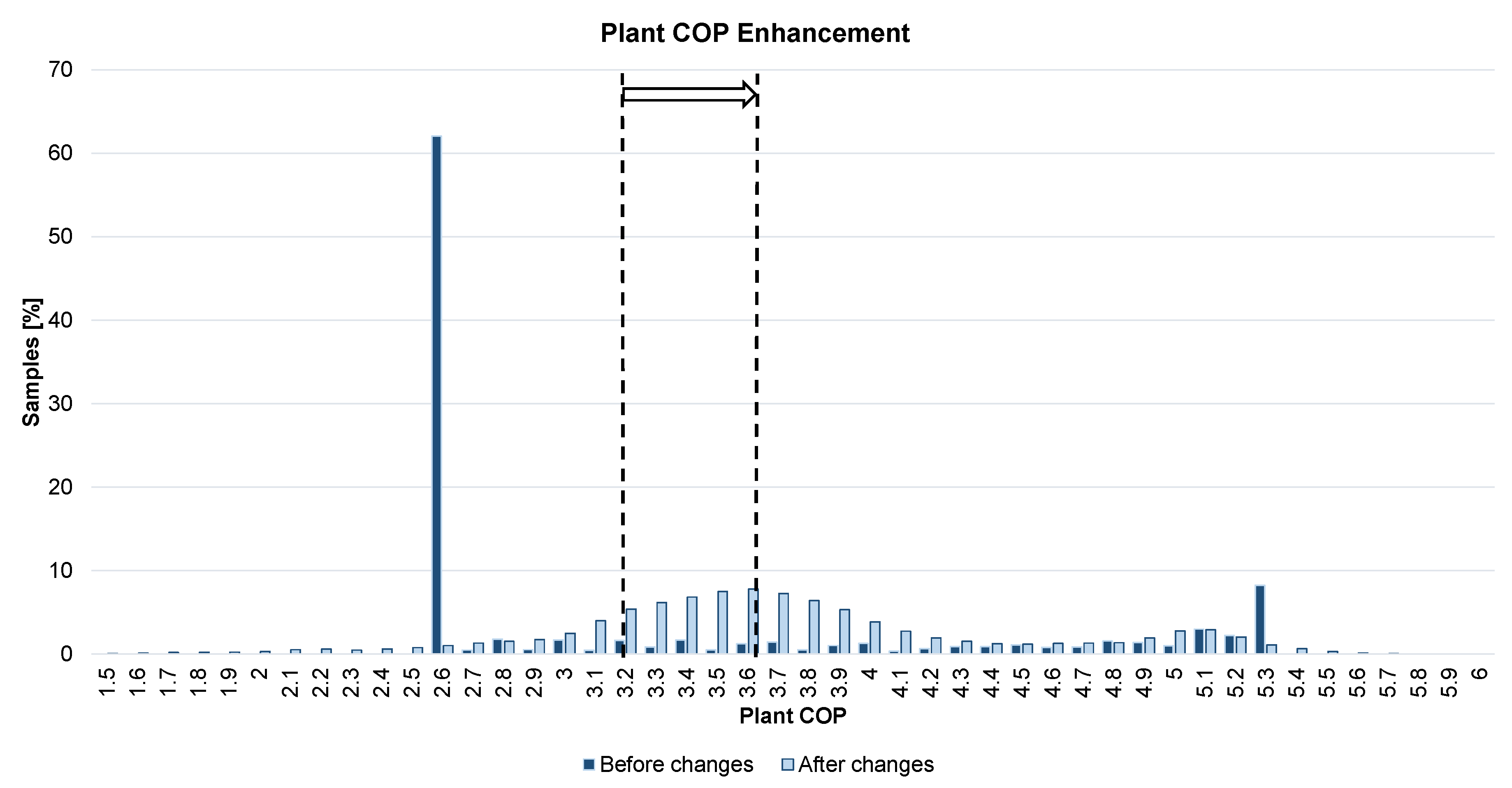
Figure 13 displays both histograms, before and after the changes. Considering all the exposed modifications and new management strategies, the plant performance has been increased from 3.2 to 3.65, i.e., an efficiency enhancement of 12.33%. It can be pointed out that the plant COP before changes remained a long time around 2.6.
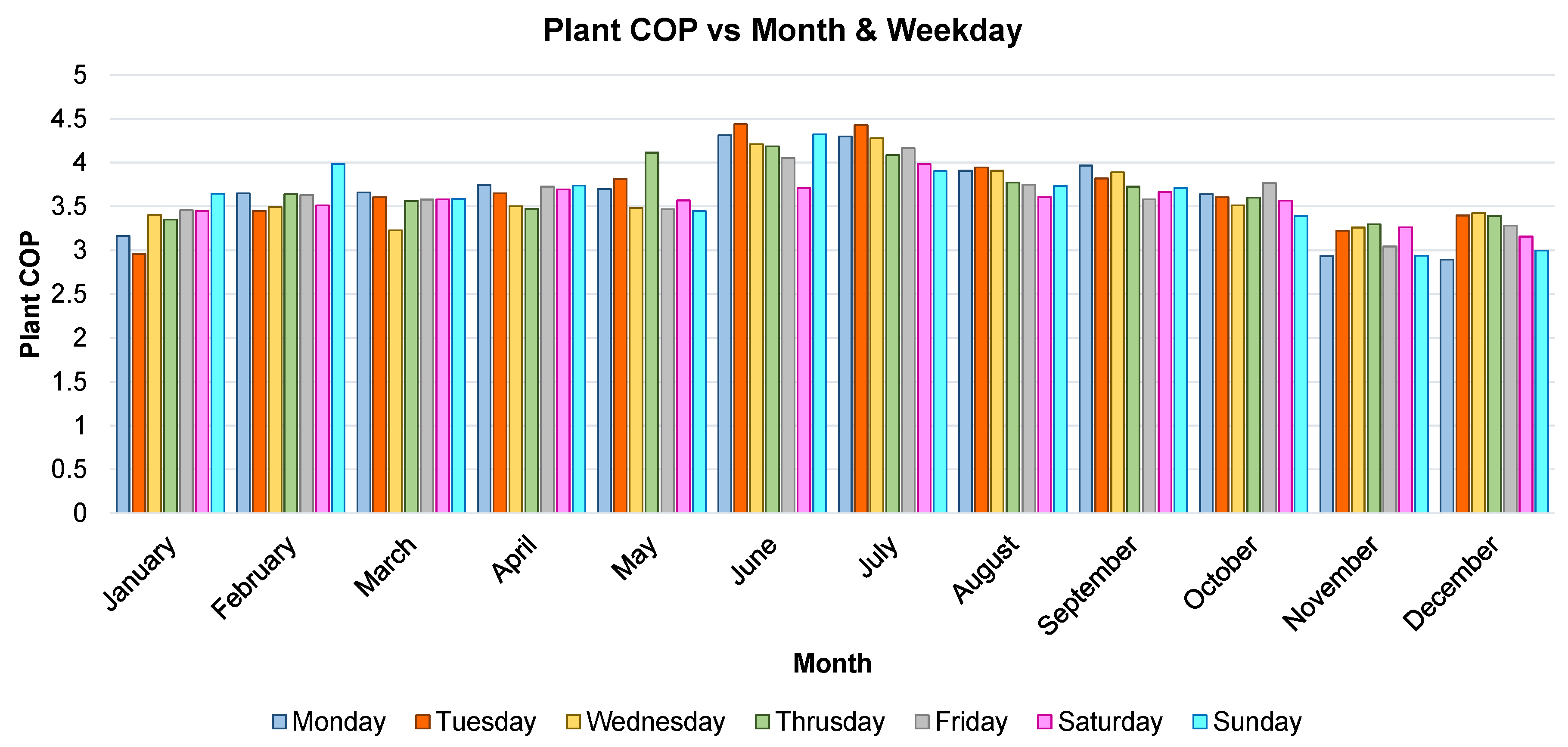
Before applying the proposed approach and deploying efficient management rules, air-cooled chillers were running a short time compared to water-cooled chillers, due to unsteady operations and electricity peak demands. Thus, water-cooled chillers were used longer, even with low cooling demands (below 1143 KW), in order to guarantee cooling supply. In this case, the chiller load ratio was the lowest possible, i.e., 0.5, often being the cooling production higher than the demand. This caused a decrease of chilled water temperature and, sometimes, a temporal chiller stop for overproduction. On the other side, there were several COP values around 5.3, corresponding to high cooling loads in summer, when water-cooled chillers run at maximum load, and a no air-cooled chiller is started in order to avoid electricity peak demands. The distribution of the plant COP after the changes is much more uniform, varying between 3.6 (influenced by air-cooled chillers operation) and 5.1 (influenced by water-cooled chillers operation). Figure 14 shows the average plant COP for each month and weekday of studied period (after changes). It varies slightly from winter to summer season according to the chiller type running. On Monday and Tuesday, the COP is usually higher due to huge cooling loads.
Our proposal takes advantage of real past data from the chillers and the plant, instead of using simulated data. Moreover, it can be deployed into conventional controllers since the rule-based management system requires low computational resources. Therefore, it is not necessary to substitute the existing hardware in the building. On the other hand, the addition of more data in subsequent years would improve the coverage, providing incremental improvements in efficiency to the plant operation.
One drawback of the proposed methodology is that it is not a completely automatic method to convert the knowledge extracted from the data analysis of the chillers and plant into management rules. Another limitation is that the iterative application of the proposed approach only provides incremental improvements to the system operation but does not guarantee an optimal result. Furthermore, the presence of a data science expert in the process would be beneficial for its correct application.
7. Conclusions
In this paper, a comprehensive methodology for improving the efficiency in multiple-chiller plants has been proposed. This methodology is based on a data analysis of the operation of the chillers and the overall plant, using real data instead of simulations. The proposed data analyses highlight relevant information by applying aggregation, filtering and data projection. Using the knowledge extracted specifically from the plant, control parameters of the chillers can be adjusted and management rules can be defined or tuned. The aim is to achieve an efficient management of the plant, without the need of incorporating cutting-edge controllers, since the management rules obtained through the proposed approach can be easily deployed in existing controllers.
The proposed methodology has been applied on a real chiller plant at the Hospital of León (Spain). Data analyses have helped to understand the operation of each chiller and the plant with regard to a chiller load ratio or outdoor temperature, which are variables that affect the efficiency of cooling production systems. The extracted knowledge about chiller performance has enabled the adjustment of internal control parameters and setpoints, detect faults and inefficient operations and define management rules, whereas the knowledge about the plant has allowed us to redefine and tune some rules. As a result, noteworthy enhancements on efficiency have been obtained after applying that methodology. In this sense, chiller COPs (especially for air-cooled chillers) and the overall plant COP (12.33% higher) have been increased. This implied an electricity savings of 380,000 KWh during the year studied at the Hospital building.
The main limitations of the proposed methodology have been discussed in the paper. On the one hand, the extracted knowledge is not automatically converted into management rules. On the other hand, our approach does not guarantee an optimal result, so iterative applications of the approach will be required.
As future work, new data from subsequent time periods (one year) will be analyzed in order to redefine or tune the management rules, evaluating the incremental improvement in efficiency provided by the approach. Furthermore, a dynamic global optimization approach will be applied, in order to compare it with our methodology in terms of efficiency, resources and computational cost.
Author Contributions
Conceptualization, S.A. and M.D.; methodology, S.A. and A.M.; software, S.A. and A.M.; validation, M.Á.P. and P.R.; formal analysis, S.A.; investigation, S.A., A.M. and M.Á.P.; data curation, S.A. and A.M.; writing—original draft preparation, S.A. and A.M.; writing—review and editing, M.Á.P. and P.R.; visualization, J.J.F. and P.R.; supervision, J.J.F. and M.D.; project administration, M.D.; funding acquisition, M.D.
Funding
This research was funded by the Spanish Ministerio de Ciencia e Innovación and the European FEDER under project CICYT DPI2015-69891-C2-1-R/2-R.
Conflicts of Interest
The authors declare no conflict of interest.
Abbreviations
The following abbreviations are used in this manuscript:
| HVAC | Heating, Ventilating and Air Conditioning |
| COP | Coefficient of Performance |
| EEI | Energy Efficiency Indicator |
| EER | Energy Efficiency Ratio |
| SCOP | Seasonal Coefficient of Performance |
| SEER | Seasonal Energy Efficiency Ratio |
| IPLV | Integrated Part Load Value |
| BMS | Building Management System |
| EEV | Electronic Expansion Valve |
| VAV | Variable Air Volume |
| PMS | Plant Manager Software |
References
- Pérez-Lombard, L.; Ortiz, J.; Pout, C. A review on buildings energy consumption information. Energy Build. 2008, 40, 394–398. [Google Scholar] [CrossRef]
- Perez-Lombard, L.; Ortiz, J.; Maestre, I.R. The map of energy flow in HVAC systems. Appl. Energy 2011, 88, 5020–5031. [Google Scholar] [CrossRef]
- Chung, M.; Park, H.C. Comparison of building energy demand for hotels, hospitals, and offices in Korea. Energy 2015, 92 Pt 3, 383–393. [Google Scholar] [CrossRef]
- Teke, A.; Timur, O. Assessing the energy efficiency improvement potentials of HVAC systems considering economic and environmental aspects at the hospitals. Renew. Sustain. Energy Rev. 2014, 33, 224–235. [Google Scholar] [CrossRef]
- Campuzano-Cervantes, J.; Meléndez-Pertuz, F.; Núñez-Perez, B.; Simancas-García, J. Electronic monitoring system of displacement of extension tubes for the expansion joint. Revista Iberoamericana Automática Informática Industrial RIAI 2017, 14, 268–278. [Google Scholar] [CrossRef]
- Chua, K.; Chou, S.; Yang, W.; Yan, J. Achieving better energy-efficient air conditioning—A review of technologies and strategies. Appl. Energy 2013, 104, 87–104. [Google Scholar] [CrossRef]
- Yu, F.; Chan, K. Improved energy management of chiller systems by multivariate and data envelopment analyses. Appl. Energy 2012, 92, 168–174. [Google Scholar] [CrossRef]
- Do, H.; Cetin, K.S. Data-Driven Evaluation of Residential HVAC System Efficiency Using Energy and Environmental Data. Energies 2019, 12, 188. [Google Scholar] [CrossRef]
- Peña, M.; Biscarri, F.; Guerrero, J.I.; Monedero, I.; León, C. Rule-based system to detect energy efficiency anomalies in smart buildings, a data mining approach. Expert Syst. Appl. 2016, 56, 242–255. [Google Scholar] [CrossRef]
- Kim, H.; Stumpf, A.; Kim, W. Analysis of an energy efficient building design through data mining approach. Autom. Constr. 2011, 20, 37–43. [Google Scholar] [CrossRef]
- Hong, T.; Yang, L.; Hill, D.; Feng, W. Data and analytics to inform energy retrofit of high performance buildings. Appl. Energy 2014, 126, 90–106. [Google Scholar] [CrossRef] [Green Version]
- Ahmad, M.W.; Mourshed, M.; Rezgui, Y. Trees vs Neurons: Comparison between random forest and ANN for high-resolution prediction of building energy consumption. Energy Build. 2017, 147, 77–89. [Google Scholar] [CrossRef]
- Lin, Y.; Zhou, S.; Yang, W.; Shi, L.; Li, C.Q. Development of Building Thermal Load and Discomfort Degree Hour Prediction Models Using Data Mining Approaches. Energies 2018, 11, 1570. [Google Scholar] [CrossRef]
- Zeng, Y.; Zhang, Z.; Kusiak, A. Predictive modeling and optimization of a multi-zone HVAC system with data mining and firefly algorithms. Energy 2015, 86, 393–402. [Google Scholar] [CrossRef]
- Afram, A.; Janabi-Sharifi, F. Review of modeling methods for HVAC systems. Appl. Therm. Eng. 2014, 67, 507–519. [Google Scholar] [CrossRef]
- Alves, O.; Monteiro, E.; Brito, P.; Romano, P. Measurement and classification of energy efficiency in HVAC systems. Energy Build. 2016, 130, 408–419. [Google Scholar] [CrossRef]
- Yu, F.; Chan, K. Experimental determination of the energy efficiency of an air-cooled chiller under part load conditions. Energy 2005, 30, 1747–1758. [Google Scholar] [CrossRef]
- Yu, F.; Chan, K. Part load performance of air-cooled centrifugal chillers with variable speed condenser fan control. Build. Environ. 2007, 42, 3816–3829. [Google Scholar] [CrossRef]
- Kabeel, A.; El-Samadony, Y.; Khiera, M. Performance evaluation of energy efficient evaporatively air-cooled chiller. Appl. Therm. Eng. 2017, 122, 204–213. [Google Scholar] [CrossRef]
- Weng, T.; Agarwal, Y. From Buildings to Smart Buildings—Sensing and Actuation to Improve Energy Efficiency. IEEE Des. Test Comput. 2012, 29, 36–44. [Google Scholar] [CrossRef]
- Oldewurtel, F.; Parisio, A.; Jones, C.N.; Gyalistras, D.; Gwerder, M.; Stauch, V.; Lehmann, B.; Morari, M. Use of model predictive control and weather forecasts for energy efficient building climate control. Energy Build. 2012, 45, 15–27. [Google Scholar] [CrossRef] [Green Version]
- Mahmoud, M.S. Multilevel Systems Control and Applications: A Survey. IEEE Trans. Syst. Man Cybern. 1977, 7, 125–143. [Google Scholar] [CrossRef]
- Findeisen, W.; Bailey, F.N.; Bryds, M.; Malinowski, K.; Tatjewski, P.; Wozniak, A. Control and Coordination in Hierarchical Systems, 1st ed.; John Wiley & Sons: Hoboken, NJ, USA, 1980; p. 478. [Google Scholar]
- Figueiredo, J.; da Costa, J.S. A SCADA system for energy management in intelligent buildings. Energy Build. 2012, 49, 85–98. [Google Scholar] [CrossRef] [Green Version]
- Li, Z.; Huang, G.; Sun, Y. Stochastic chiller sequencing control. Energy Build. 2014, 84, 203–213. [Google Scholar] [CrossRef]
- Shan, K.; Wang, S.; ce Gao, D.; Xiao, F. Development and validation of an effective and robust chiller sequence control strategy using data-driven models. Autom. Constr. 2016, 65, 78–85. [Google Scholar] [CrossRef]
- Sun, Y.; Wang, S.; Huang, G. Chiller sequencing control with enhanced robustness for energy efficient operation. Energy Build. 2009, 41, 1246–1255. [Google Scholar] [CrossRef]
- Chan, K.; Yu, F. Applying condensing-temperature control in air-cooled reciprocating water chillers for energy efficiency. Appl. Energy 2002, 72, 565–581. [Google Scholar] [CrossRef]
- Yu, F.; Chan, K. Advanced control of condensing temperature for enhancing the operating efficiency of air-cooled chillers. Build. Environ. 2005, 40, 727–737. [Google Scholar] [CrossRef]
- Seem, J.E. Using intelligent data analysis to detect abnormal energy consumption in buildings. Energy Build. 2007, 39, 52–58. [Google Scholar] [CrossRef]
- Thangavelu, S.R.; Myat, A.; Khambadkone, A. Energy optimization methodology of multi-chiller plant in commercial buildings. Energy 2017, 123, 64–76. [Google Scholar] [CrossRef]
- Beghi, A.; Cecchinato, L.; Cosi, G.; Rampazzo, M. A PSO-based algorithm for optimal multiple chiller systems operation. Appl. Therm. Eng. 2012, 32, 31–40. [Google Scholar] [CrossRef]
- Ardakani, A.J.; Ardakani, F.F.; Hosseinian, S. A novel approach for optimal chiller loading using particle swarm optimization. Energy Build. 2008, 40, 2177–2187. [Google Scholar] [CrossRef]
- Hartman, T. Designing Efficient Systems With the Equal Marginal Performance Principle. ASHRAE J. 2005, 47, 64–70. [Google Scholar]
- Mařík, K.; Rojíček, J.; Stluka, P.; Vass, J. Advanced HVAC Control: Theory vs. Reality. IFAC Proc. Volumes 2011, 44, 3108–3113. [Google Scholar] [CrossRef]
- Wang, S.; Ma, Z. Supervisory and Optimal Control of Building HVAC Systems: A Review. HVAC R Res. 2008, 14, 3–32. [Google Scholar] [CrossRef]
- Díaz, I.; Cuadrado, A.A.; Pérez, D.; Domínguez, M.; Alonso, S.; Prada, M.A. Energy analytics in public buildings using interactive histograms. Energy Build. 2017, 134, 94–104. [Google Scholar] [CrossRef]
- Morán, A.; Fuertes, J.J.; Domínguez, M.; Prada, M.A.; Alonso, S.; Barrientos, P. Analysis of electricity bills using visual continuous maps. Neural Comput. Appl. 2013, 23, 645–655. [Google Scholar] [CrossRef]
- Behrooz, F.; Mariun, N.; Marhaban, M.H.; Mohd Radzi, M.A.; Ramli, A.R. Review of Control Techniques for HVAC Systems—Nonlinearity Approaches Based on Fuzzy Cognitive Maps. Energies 2018, 11, 495. [Google Scholar] [CrossRef]
Figure 1.
Methodology for extracting knowledge and enhancing efficiency in Chiller Plants.

Figure 2.
Chiller plant at the Hospital of León.

Figure 3.
Evolution of COP with chiller load.

Figure 4.
Evolution of COP with outdoor temperature.

Figure 5.
Architecture of the plant manager software.

Figure 6.
Chiller up and down management strategies.

Figure 7.
Analysis of cooling demand.

Figure 8.
Plant COP vs. Daily average outdoor temperature.

Figure 9.
Plant COP vs. Cooling Load.

Figure 10.
Contribution of each chiller to cooling load of the building.

Figure 11.
Histogram of chiller COP before and after control changes.

Figure 12.
Comparison of chillers in terms of COP.

Figure 13.
Histogram of plant COP before and after chiller plant changes.

Figure 14.
Plant COP each month and weekday after changes.


Table 1.
Chiller data overview.
| Water-Cooled Chillers | Air-Cooled Chillers | |
|---|---|---|
| Number | 2 | 5 |
| Compressors | 1 | 3 |
| Cooling power [kW] | 2286 | 1407 |
| Electric power [kW] | 367 | 327 |
| Primary Pump [kW] | 18.5 | 15 |
| Fans [kW] | 18.5 | 24 |
| Cooling Tower Pump [kW] | 30 | - |
| Compressor COP | 6.23 | 4.30 |
| Overall COP | 5.27 | 3.84 |
Table 2.
Main changes in the air-cooled chiller configuration.
| Parameter | Value Before | Value After |
|---|---|---|
| Water setpoint [C] | 7 | 6 |
| Control zone [C] | ||
| Delay [s] | 30 | 300 |
| Rate of Change [C/s] | ||
| Slide [%] | 50–100 | 65–100 |
| Adjust [%] | 1–5 | 2–10 |
| Deadband [A] | ||
| Load and unload pulses [s] | 0.2 | 0.8 |
| Pulse delay [s] | 1 | 5 |
| Condensing control range [KPa] | 758–896 | 758–1241 |
| Unsafe suction warning [KPa] | 138 | 34 |
Table 3.
Stage up/down rules set.
| Conditions | Actions | Opposite Actions |
|---|---|---|
| If | Then | Else |
| (CoolingLoad > ChillerCapacity) & | ||
| & (ChillerLoad > 0.9) | ChillerUp | - |
| (CoolingLoad < ChillerCapacity) & | ||
| & (ChillerLoad < 0.7) & (NoChillersOn > 1) | ChillerDown | - |
| NoChillersOn == 0 | ChillerUp | - |
| RelativeRunningHours > RotationSp | ChillerDown | - |
| (SupplyTemp > 10 C) | (ReturnTemp > 14 C) | ChillerUp | - |
| (SupplyTemp < 6 C) | (ReturnTemp < 10 C) | ChillerDown | - |
Table 4.
Delimiting rule set.
| Conditions | Actions | Opposite Actions |
|---|---|---|
| If | Then | Else |
| (AvgOutdoorTemp > 16 C) | WCCyUp | WCCyDown |
| (AvgOutdoorTemp < 12 C) | ACCxUp | ACCxDown |
Table 5.
Exclusion rule set.
| Conditions | Actions | Opposite Actions |
|---|---|---|
| If | Then | Else |
| ChillerEnable == 1 | ChillerUp/Down | Up/Down Disable |
| ChillerAlarm == 1 | Up/Down Disable | ChillerUp/Down |
| PowerDemand > 1300 KW | UpDisable | ChillerUp |
| IdleCapacity < StopChillerLoad | Down Disable | ChillerDown |
Table 6.
Criteria and order for sorting chillers.
| Criterion | Asc./des. Order | |
|---|---|---|
| Chiller up? | ||
| 1 | Chiller Priority (P) | Ascending |
| 2 | Chiller COP (COP) | Descending |
| 3 | Total Running Hours (TRH) | Ascending |
| 4 | Start Count (SC) | Ascending |
| 5 | Hours From Last Stop (HLS) | Descending |
| Chiller down? | ||
| 11 | Chiller Load (CLR) | Ascending |
| 12 | Relative Running Hours (RRH) | Descending |
| 13 | Chiller COP (COP) | Ascending |
Table 7.
Updated rules set.
| Conditions | Actions | Opposite Actions |
|---|---|---|
| If | Then | Else |
| (CoolingLoad < ChillerCapacity) & | ||
| & (ChillerLoad < 0.6) & (NoChillersOn > 1) | ChillerDown | - |
| Winter == 1 | ACCxUp | ACCxDown |
| Summer == 1 | WCCyUp | WCCyDown |
| ((Spring == 1) | (Autumn == 1)) & | ||
| & (AvgOutdoorTemp < 14 C) | ACCxUp | ACCxDown |
| ((Spring == 1) | (Autumn == 1)) & | ||
| & (AvgOutdoorTemp > 14 C) | WCCyUp | WCCyDown |
| (CoolingLoad > 1500 KW) & (Hour < 10 h) | WCCyUp | ACCxDown |
| (CoolingLoad < 900 KW) & (Hour > 22 h) | ACCxUp | WCCyDown |
Table 8.
Efficiency results for all chillers.
| Chiller | COP Before | COP After | Variation [%] |
|---|---|---|---|
| ACC1 | 3.18 | 3.76 | +18.35 |
| ACC2 | - | - | - |
| ACC3 | 3.04 | 3.48 | +14.28 |
| ACC4 | 2.80 | 3.17 | +12.99 |
| ACC5 | 2.91 | 3.39 | +16.30 |
| WCC1 | 4.15 | 4.19 | +0.96 |
| WCC2 | 4.08 | 4.13 | +1.22 |
© 2019 by the authors. Licensee MDPI, Basel, Switzerland. This article is an open access article distributed under the terms and conditions of the Creative Commons Attribution (CC BY) license (http://creativecommons.org/licenses/by/4.0/).
Share and Cite
MDPI and ACS Style
Alonso, S.; Morán, A.; Prada, M.Á.; Reguera, P.; Fuertes, J.J.; Domínguez, M. A Data-Driven Approach for Enhancing the Efficiency in Chiller Plants: A Hospital Case Study. Energies 2019, 12, 827. https://doi.org/10.3390/en12050827
AMA Style
Alonso S, Morán A, Prada MÁ, Reguera P, Fuertes JJ, Domínguez M. A Data-Driven Approach for Enhancing the Efficiency in Chiller Plants: A Hospital Case Study. Energies. 2019; 12(5):827. https://doi.org/10.3390/en12050827
Chicago/Turabian StyleAlonso, Serafín, Antonio Morán, Miguel Ángel Prada, Perfecto Reguera, Juan José Fuertes, and Manuel Domínguez. 2019. "A Data-Driven Approach for Enhancing the Efficiency in Chiller Plants: A Hospital Case Study" Energies 12, no. 5: 827. https://doi.org/10.3390/en12050827
Note that from the first issue of 2016, this journal uses article numbers instead of page numbers. See further details here.