Stochastic Optimization for Integration of Renewable Energy Technologies in District Energy Systems for Cost-Effective Use

Abstract

Stochastic optimization of a district energy system (DES) is investigated with renewable energy systems integration and uncertainty analysis to meet all three major types of energy consumption: electricity, heating, and cooling. A district of buildings on the campus of the University of Utah is used as a case study for the analysis. The proposed DES incorporates solar photovoltaics (PV) and wind turbines for power generation along with using the existing electrical grid. A combined heat and power (CHP) system provides the DES with power generation and thermal energy for heating. Natural gas boilers supply the remaining heating demand and electricity is used to run all of the cooling equipment. A Monte Carlo study is used to analyze the stochastic power generation from the renewable energy resources in the DES. The optimization of the DES is performed with the Particle Swarm Optimization (PSO) algorithm based on a day-ahead model. The objective of the optimization is to minimize the operating cost of the DES. The results of the study suggest that the proposed DES can achieve operating cost reductions (approximately 10% reduction with respect to the current system). The uncertainty of energy loads and power generation from renewable energy resources heavily affects the operating cost. The statistical approach shows the potential to identify probable operating costs at different time periods, which can be useful for facility managers to evaluate the operating costs of their DES.

1. Introduction

Power generation from distributed energy resources has become increasingly popular [1]. Traditional power generation is often associated with large-scale power plants [2], but distributed power generation tends to occur on smaller scales and is located near the end users. The introduction of distributed generation allows the local energy demand to be less dependent on the grid [3] and may provide additional efficiencies by using local energy resources. Renewable energy systems in recent years have been considered within distributed generation systems [4]. One of the advantages of renewable energy systems is that they can be configured in various system sizes to meet the local energy demand [5].

The options for integrating renewable energy systems into district energy systems (DES) vary depending on the location and the objective of the DES [6]. The integration of renewable energy systems into DES has been actively explored in recent literature. Various renewable energy technologies are utilized in DES, ranging from small scale to large scale [7]. The types of technology are also dependent on the location of the DES [8]. In other words, the availability of local renewable energy resources determines the type of renewable energy systems which can be employed in that area [9]. Solar and wind power are the two most popular types of renewable energy technologies integrated into DES [10]. Furthermore, geothermal, biomass, and hydropower are also attractive options for locations containing the respective energy resources [11]. Other types of distributed energy systems such as combined heat and power (CHP) are also used for DES planning [12].

Power generation of solar and wind energy systems can be interrupted due to the intermittency and uncertainty of solar irradiation [13] and wind speed [14]. Mathematical models have been developed to address the intermittency of renewable power generation in DES [15]. For example, Parisio et al. proposed a Robust Optimization technique to control energy carriers into an energy hub [16]. Evins et al. utilized Mixed-integer Linear Programming to address operational constraints [17]. Mavromatidis et al. introduced a two-stage stochastic programming approach to optimal design of distributed energy systems [18]. Jabbari-Sabet et al. used Particle Swarm Optimization and Unit Commitment to solve for DES operation and management of a 10-bus system in the day-ahead model [19]. Fioriti et al. investigated a hybrid minigrid under load and renewable generation uncertainty [20]. The results from these studies show that stochastic optimization can be used to address the uncertainties associated with DES.

There are a number of ways to incorporate stochasticity in the simulation and optimization of renewable energy systems. In recent literature, the uncertainties of power generation from renewable energy systems have been investigated for meeting the electricity demand [21], heating demand [22], and cooling demand [23]. Najibi et al. investigated stochastic scheduling of renewable energy resources to meet the electricity demand under uncertainties of solar photovoltaics (PV) power generation [24]. Similarly, Nikmehr et al. studied the operating cost optimization of a network of energy hubs to fulfill the electricity demand [25]. Balaman and Selim focused on meeting the heating demand in a heating district system [26]. Lu et al. presented a modeling solution to coordinate dispatch of a multi-energy system with district heating network [27]. Comparatively, Sameti and Haghighat studied optimization methods for a cooling network together with a district heating network [28]. Furthermore, Gang et al. presented an uncertainty-based design optimization for stand-lone district cooling systems [29]. Overall, these DES planning studies are mostly focused on meeting one of the three major energy demands, with electricity as the main focus.

There are limited studies on optimizing the operating cost of DES with consideration of all three major energy demands. Li et al. optimized building cooling heating and power system with consideration of uncertainty of energy demands [30]. Recently, Mavromatidis et al. incorporated uncertainty and global sensitivity analysis to optimize design of an energy hub [31]. There is a need to further investigate all three major energy use types, especially in the presence of uncertainty and global sensitivity analysis. The addition of cooling and heating demand to the analysis is important for the overall operation of the DES. This is because systems such as CHP can utilize thermal energy, which is a by-product of power generation, for fulfilling the heating demand. Furthermore, the uncertainties in power generation can impact the fulfillment of the cooling demand since cooling equipment is run by electrical power. In this work, these uncertainties can be included in the model for optimization without requiring a stochastic programming approach, in which later decision stages depend on uncertainties in earlier decision stages [32].

The novelty of this paper is to establish an optimization framework with uncertainty incorporated in terms of stochastic renewable power generation systems and stochastic energy use (loads) based on a day-ahead model to optimize the operating cost of a modeled DES and potentially reduce dependence on the grid. To address the existing gap in the literature, all three major categories of energy consumption (electricity, heating, and cooling) are considered in the presence of renewable power generation and energy usage uncertainties. These energy needs of the DES are met by a mix of renewable energy systems (solar PV and wind turbines), CHP system, energy storage, natural gas boilers, and the electrical grid.

This study uses real data from a group of existing buildings on the campus of the University of Utah as a case study. These buildings are metered to measure both the electrical and thermal energy consumption. The uncertainties of energy consumption patterns and power generation from the renewable energy resources (i.e., solar irradiation and wind speed) are analyzed based on the Monte Carlo approach. The DES is optimized with the population-based Particle Swarm Optimization (PSO) algorithm. The objective of the optimization is to minimize the operating cost of the DES on the day-ahead model.

Unlike the aforementioned works in the literature, the results from this study will lay the groundwork for the adding renewable energy systems into DES with (1) considering of all three major types of energy consumption (electricity, heating, and cooling) in buildings; (2) including of the uncertainties of energy consumption and power generation from renewable energy resources; (3) incorporating the Monte Carlo statistical approach into the population-based PSO; and (4) generating statistical distributions of the operating cost at different time periods in order to stochastically optimize for the operating cost of the DES.

2. Problem Formulation

2.1. District Energy System Description

The methodology described in this section can be applied to any DES with known electricity, heating, and cooling demands. Energy system sizes in the DES can be adjusted according to the demands of the given DES. The stochastic optimization methodology proposed in this paper is examined by utilizing a group of existing buildings on the campus of the University of Utah as a case study. The buildings are predominantly used as offices and classrooms. As previously mentioned, the chosen buildings are metered for energy usage, disaggregate into electricity, heating, and cooling. The study examines the DES on four different days of the year (20 March, 21 June, 22 September, and 21 December), which occur at the beginning of the four astronomical seasons. During these four days, offices and classrooms are open. Throughout this paper, the existing energy system (utilizing the electrical grid and natural gas) will be referred to as the current energy system. On the other hand, the modeled DES (utilizing a mixed of energy systems) will be referred to as the proposed DES. Furthermore, the non-cooling electricity load will be referred to as simply the electricity load, while the electrical energy required to run cooling equipment will be referred to as the cooling load.

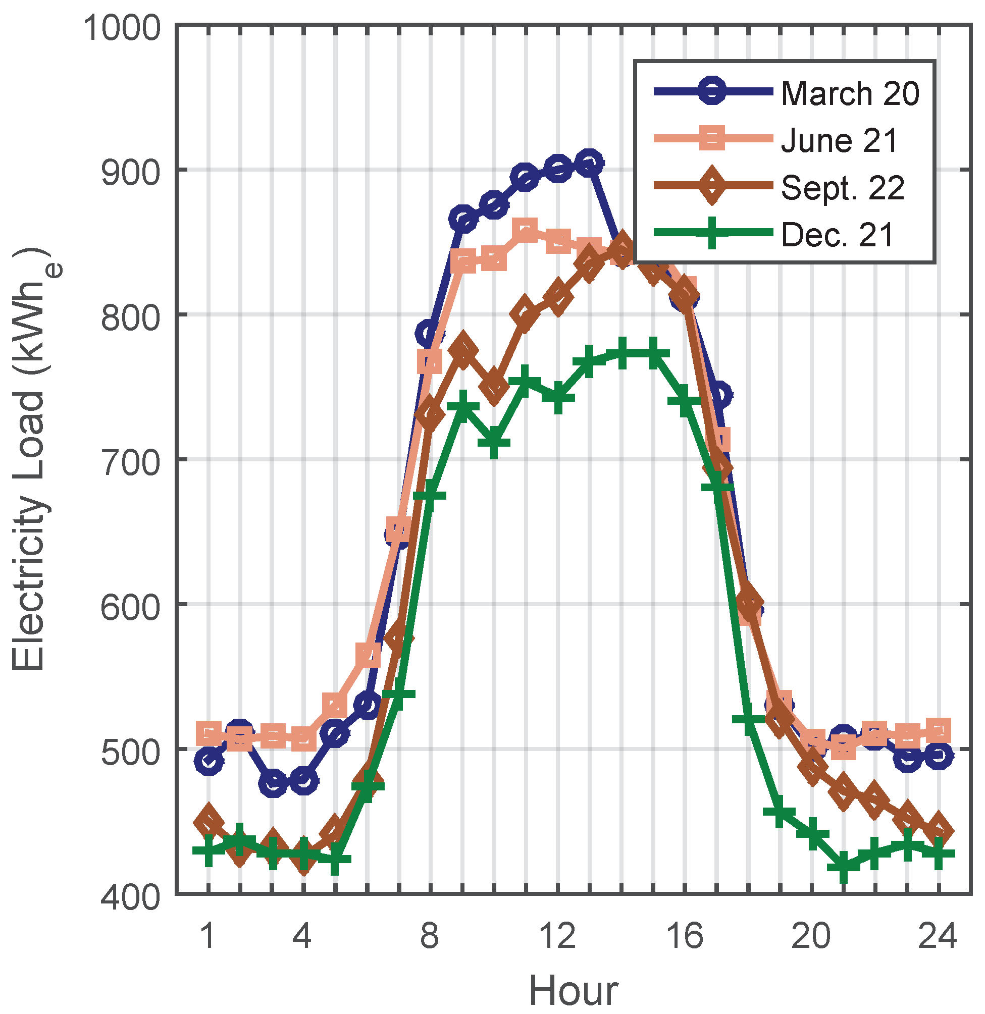
The average energy loads of the buildings comprising the proposed DES are detailed in

Table 1. Average loads on four example days.

Design Day	Electricity (kWh${}_{\mathbf{e}}$)	Heating (kWh${}_{\mathbf{t}}$)	Cooling (kWh${}_{\mathbf{t}}$)
20 March	15,747	15,243	5940
21 June	15,669	12,675	6897
22 September	14,981	14,981	4749
21 December	13,641	24,693	62

. To obtain average energy loads representing the four example days, hourly energy data is taken from 10 preceding days and 10 subsequent days to capture typical load patterns during the time of year around that particular example day. Figure 1 shows the daily energy loads of 21 June and its 20 neighboring days to illustrate the process of obtaining data for the study. Instead of using only the actual energy data for 21 June, incorporating data from neighboring days allows for a representative energy load that includes stochastic variation in the likely energy load on such an example day, which will be discussed further in Section 2.3.1. The data represents the real energy loads in 2017 and is obtained from the university’s SkySpark installation, a building analytics platform that collects building data [33]. The mean and standard deviation of each set of hourly energy data are shown in the Appendix A (

Table A1. Electricity load parameters (mean and standard deviation) on four different days.

Hour	20 March		21 June		22 September		21 December
	${\mathit{\mu }}_{\mathit{e}}$ (${\mathbf{kWh}}_{\mathbf{e}}$)	${\mathit{\sigma }}_{\mathit{e}}$ (${\mathbf{kWh}}_{\mathbf{e}}$)	${\mathit{\mu }}_{\mathit{e}}$ (${\mathbf{kWh}}_{\mathbf{e}}$)	${\mathit{\sigma }}_{\mathit{e}}$ (${\mathbf{kWh}}_{\mathbf{e}}$)	${\mathit{\mu }}_{\mathit{e}}$ (${\mathbf{kWh}}_{\mathbf{e}}$)	${\mathit{\sigma }}_{\mathit{e}}$ (${\mathbf{kWh}}_{\mathbf{e}}$)	${\mathit{\mu }}_{\mathit{e}}$ (${\mathbf{kWh}}_{\mathbf{e}}$)	${\mathit{\sigma }}_{\mathit{e}}$ (${\mathbf{kWh}}_{\mathbf{e}}$)
1	492.42	78.23	510.71	49.75	657.89	65.41	429.03	26.75
2	511.60	62.46	506.69	50.69	655.37	55.78	436.98	33.11
3	476.17	39.53	509.14	34.78	653.73	63.17	428.12	31.44
4	478.87	52.44	507.32	40.79	660.89	51.66	427.85	26.69
5	511.08	53.42	530.30	60.84	659.19	63.16	423.37	20.65
6	529.76	71.35	565.72	75.10	652.64	74.22	474.46	60.99
7	648.10	123.35	651.39	121.28	614.04	130.92	536.99	121.74
8	787.19	226.12	767.94	212.78	652.64	205.47	675.41	238.52
9	865.34	275.10	836.83	263.74	636.82	237.01	736.64	242.62
10	874.86	299.60	838.10	253.89	629.66	229.00	711.87	244.43
11	894.97	299.57	857.70	286.99	598.15	251.63	753.22	275.50
12	899.92	316.56	851.30	280.72	601.63	246.20	743.35	254.13
13	904.45	309.82	845.24	275.72	593.17	255.07	767.43	277.31
14	842.33	253.54	842.93	268.87	585.06	274.90	773.44	274.42
15	840.84	272.48	851.29	278.20	594.54	272.84	773.42	288.34
16	812.61	232.82	818.29	256.29	583.22	271.62	741.42	269.55
17	743.79	209.39	713.25	182.44	576.40	196.91	680.65	204.78
18	596.05	107.02	594.80	106.00	596.24	124.50	520.45	93.33
19	529.86	74.13	531.36	54.66	596.45	73.24	456.38	45.16
20	501.35	71.04	505.51	49.00	610.09	73.45	441.01	38.74
21	506.23	73.42	500.44	49.56	640.57	72.20	418.94	32.48
22	508.79	76.29	510.73	47.05	622.50	72.99	428.42	32.92
23	494.29	74.72	509.24	40.09	656.26	81.63	434.20	41.73
24	496.05	73.94	512.64	44.51	654.28	63.58	428.38	33.33

,

Table A2. Heating load parameters (mean and standard deviation) on four different days.

Hour	20 March		21 June		22 September		21 December
	${\mathit{\mu }}_{\mathit{h}}$ (${\mathbf{kWh}}_{\mathbf{t}}$)	${\mathit{\sigma }}_{\mathit{h}}$ (${\mathbf{kWh}}_{\mathbf{t}}$)	${\mathit{\mu }}_{\mathit{h}}$ (${\mathbf{kWh}}_{\mathbf{t}}$)	${\mathit{\sigma }}_{\mathit{h}}$ (${\mathbf{kWh}}_{\mathbf{t}}$)	${\mathit{\mu }}_{\mathit{h}}$ (${\mathbf{kWh}}_{\mathbf{t}}$)	${\mathit{\sigma }}_{\mathit{h}}$ (${\mathbf{kWh}}_{\mathbf{t}}$)	${\mathit{\mu }}_{\mathit{h}}$ (${\mathbf{kWh}}_{\mathbf{t}}$)	${\mathit{\sigma }}_{\mathit{h}}$ (${\mathbf{kWh}}_{\mathbf{t}}$)
1	697.17	100.87	550.01	141.21	657.89	83.13	1078.32	142.08
2	704.61	110.71	559.89	146.39	655.37	79.77	1080.78	139.29
3	687.97	93.11	567.40	149.00	653.73	73.07	1138.20	207.98
4	716.95	115.52	570.12	149.75	660.89	77.54	1174.89	189.36
5	704.81	106.46	577.08	153.48	659.19	78.13	1127.84	173.81
6	726.84	113.43	576.53	147.03	652.64	73.65	1082.01	150.15
7	705.36	120.04	551.37	144.82	614.04	73.01	1046.14	144.54
8	682.38	126.15	600.40	169.66	652.64	78.88	1130.84	163.64
9	659.12	105.02	544.82	142.87	636.82	80.54	1082.01	162.38
10	617.38	90.15	529.00	136.83	629.66	95.09	1052.55	161.84
11	566.44	80.83	568.69	294.81	598.15	64.24	994.99	169.91
12	547.21	73.58	522.25	155.51	601.63	66.04	960.62	154.69
13	516.04	111.26	504.86	131.79	593.17	63.71	911.11	150.71
14	590.38	160.71	482.49	120.80	585.06	69.34	929.25	123.72
15	543.12	87.06	488.63	123.65	594.54	70.31	914.65	124.07
16	573.81	119.23	481.13	121.19	583.22	64.92	930.75	132.15
17	550.89	86.23	476.29	119.45	576.40	63.66	913.29	107.82
18	558.94	96.10	474.99	120.90	596.24	74.02	963.89	123.46
19	591.54	88.92	486.38	123.28	596.45	72.37	969.89	128.04
20	617.38	110.46	490.61	129.21	610.09	88.85	1010.67	129.43
21	655.57	111.91	498.24	140.00	640.57	83.58	1032.63	147.96
22	674.87	112.51	511.07	142.23	622.50	81.68	1018.04	129.34
23	674.60	102.79	528.73	139.95	656.26	87.64	1080.92	139.95
24	679.37	121.17	533.91	148.33	654.28	76.48	1068.37	139.65

and

Table A3. Cooling load parameters (mean and standard deviation) on four different days.

Hour	20 March		21 June		22 September		21 December
	${\mathit{\mu }}_{\mathit{c}}$ (${\mathbf{kWh}}_{\mathbf{t}}$)	${\mathit{\sigma }}_{\mathit{c}}$ (${\mathbf{kWh}}_{\mathbf{t}}$)	${\mathit{\mu }}_{\mathit{c}}$ (${\mathbf{kWh}}_{\mathbf{t}}$)	${\mathit{\sigma }}_{\mathit{c}}$ (${\mathbf{kWh}}_{\mathbf{t}}$)	${\mathit{\mu }}_{\mathit{c}}$ (${\mathbf{kWh}}_{\mathbf{t}}$)	${\mathit{\sigma }}_{\mathit{c}}$ (${\mathbf{kWh}}_{\mathbf{t}}$)	${\mathit{\mu }}_{\mathit{c}}$ (${\mathbf{kWh}}_{\mathbf{t}}$)	${\mathit{\sigma }}_{\mathit{c}}$ (${\mathbf{kWh}}_{\mathbf{t}}$)
1	257.61	210.82	280.32	96.75	141.85	109.30	2.11	4.25
2	202.13	150.68	265.69	113.81	138.81	111.10	1.40	3.11
3	192.69	234.93	269.10	95.35	155.52	116.62	0.95	1.82
4	195.11	167.76	261.36	88.47	142.87	113.81	0.68	1.90
5	227.84	262.97	249.53	95.69	136.87	107.31	0.85	2.27
6	174.00	180.22	210.45	95.87	127.32	106.06	0.82	2.22
7	173.08	221.68	188.80	92.72	130.49	118.43	0.68	1.78
8	149.32	146.07	194.46	104.96	134.89	119.86	0.41	1.42
9	202.58	270.27	189.14	99.56	146.96	130.81	0.68	2.03
10	212.18	216.60	227.16	107.62	161.56	120.35	0.51	1.73
11	288.54	248.76	281.14	109.30	211.44	138.68	0.92	1.96
12	298.12	305.31	341.87	210.20	261.47	135.18	0.72	1.85
13	270.16	208.78	372.59	192.94	225.94	172.15	19.27	63.33
14	279.64	219.37	887.00	224.44	343.47	239.39	5.73	20.31
15	332.83	210.79	893.92	181.93	282.54	177.26	2.22	6.23
16	293.93	221.84	370.38	223.22	311.18	273.30	2.32	6.05
17	327.79	262.04	349.64	197.39	272.99	194.18	6.38	9.85
18	323.52	228.54	325.64	231.39	258.33	195.67	4.30	8.34
19	310.84	161.43	359.33	187.46	233.37	114.49	2.35	4.50
20	261.70	138.12	290.11	144.77	210.35	101.01	1.23	2.31
21	296.96	167.39	293.83	121.65	215.06	147.97	3.75	2.60
22	249.67	146.55	262.00	86.49	206.98	186.12	1.36	2.23
23	216.01	161.22	254.58	124.55	155.56	114.35	0.92	1.95
24	203.84	147.97	316.67	163.50	143.28	116.88	1.19	2.10

). The average values are plotted in Figure 2, Figure 3 and Figure 4. The daily electricity load is consistent while the daily heating and cooling loads vary throughout the year. The DES is located at Salt Lake City, UT, which is part of American Society of Heating, Refrigerating and Air-Conditioning Engineers (ASHRAE) climate zone 5 (i.e., cool and dry) [34]. Buildings in this climate zone typically exhibit considerable heating and cooling demands in winter and summer, respectively.

2.2. Proposed District Energy System

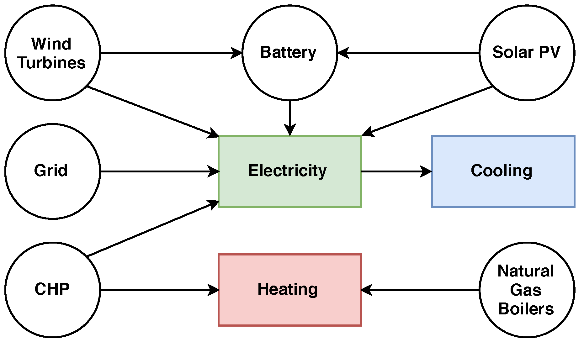
The DES utilizes the local renewable energy resources for power generation to reduce the dependence on the electrical grid. The diagram of the proposed DES is illustrated in Figure 5. In particular, solar PV and wind power are the two renewable power generation sources integrated into the DES. The National Renewable Energy Laboratory (NREL) provides hourly data over the last 15 years for wind speed [35] and solar irradiation [36] at the study location of Salt Lake City, UT, USA (40.766837, −111.846920). In addition to renewable power generation, a gas-fired microturbine CHP system is used to provide power generation during times of electrical demand when solar PV and wind power is inadequate to meet the electricity loads. A battery system is also implemented to store unconsumed renewable energy for use at a later time. Additionally, the power generated from these resources will be used to run cooling equipment to meet the cooling demand. The system will recover thermal energy from the CHP system in addition to using natural gas boilers to meet the heating demand. The technical specifications of these systems are listed in

Table 2. Energy system specifications for the proposed DES.

Energy System	Specifications
Solar PV [37]	Capacity: 400 kW
	Efficiency: 15%
	Performance ratio: 75%
	Dimension: 1.6 m2 for a 200 W panel
	Tilt angle: 40.5${}^{\circ }$
Wind Turbine [37]	Capacity: 400 kW
	Rotor diameter: 25 m
	Cut-in speed: 2.7 m/s
	Cut-out speed: 25 m/s
	Rated speed: 12 m/s
CHP [38]	Capacity: 300 kW
	Technology: microturbine
	Power to heat ratio: 0.6
	Effective electrical efficiency: 55%
	Overall CHP efficiency: 65%
Battery [37]	Capacity: 100 kW
	Charging/discharging efficiency: 90%
	Depth of discharge: 90%
Boiler [39]	Capacity: 500 MBtu/h (146.5 kW)
	Fuel-to-steam efficiency: 85%
	Fuel: natural gas

. The system sizes for the simulations presented here were chosen based on the energy demands of the buildings and the availability of renewable energy resources in the area. Different design choices will affect the on-site generation and ultimately the operating cost of the DES.

2.3. Mathematical Model

The objective of the mathematical model is to minimize the operating cost of the DES, which consists of the operating costs of the solar PV panels, wind turbines, battery system, CHP system, natural gas boilers, and electricity purchased from the grid. This work assumes that these systems are already installed. The operating and maintenance costs of these devices can be less significant to decision makers as their variation with energy output is small. Their capital costs can be found in Appendix B. All of the variables in the mathematical model are hourly because the solar irradiation, wind speed, and energy loads are provided as hourly data. The objective function of the operating cost is detailed as follows:

$$\begin{array}{c}\hfill \mathit{Min}f\left(X\right)=\mathit{Min}\sum _{t=1}^{T}Cos{t}^t=\mathit{Min}\sum _{t=1}^T\{\sum _{i=1}^{N_g}\left[u_i\left(t\right)E_{G,i}\left(t\right)C_{G,i}\left(t\right)\right]\\ \hfill +\sum _{j=1}^{N_s}\left[u_j\left(t\right)E_{S,j}\left(t\right)C_{S,j}\left(t\right)\right]+\sum _{k=1}^{N_h}\left[u_k\left(t\right)Q_{H,k}\left(t\right)C_{H,k}\left(t\right)\right]+u_l\left(t\right)E_{grid}\left(t\right)C_{grid}\left(t\right)\}.\end{array}$$

(1)

For electricity generation (the first term in brackets on the right-hand side of Equation (1)): $N_g$ is the number of generating units, $u_i$ is the state of the ith unit (ON = 1, OFF = 0), $E_{G,i}$ is the electricity generation of the ith generating unit, and $C_{G,i}$ is the ith generating unit cost. The generating units consists of on-site generation from solar, wind, and CHP. For energy storage (the second term in brackets on the right-hand side of Equation (1)): $N_s$ is the number of energy storage devices, $u_j$ is the state of the jth unit (ON = 1, OFF = 0), $E_{S,j}$ is the energy capacity of the jth energy storage device, and $C_{S,j}$ is the jth storage device cost. For thermal heating devices, including gas-fired boilers (the third term in brackets on the right-hand side of Equation (1)): $N_h$ is the number of heating devices, $u_k$ is the state of the kth unit (ON = 1, OFF = 0), $Q_{H,j}$ is the thermal energy of the kth heating device, and $C_{H,k}$ is the kth heating unit cost. When purchasing electricity from the grid, $u_l$ is the state of sending/receiving electricity from the utility (ON = 1, OFF = 0), $E_{grid}$ is the electricity purchased (or exported) from (or to) the utility, and $C_{grid}$ is the energy unit cost purchased from the utility.

The following equations break down the operating costs and constraints of all energy devices used in the proposed DES. The operating costs from renewable energy resources (i.e., solar and wind power) come from the operating & maintenance (O&M) costs of these systems. The fuel costs are zero since the fuels for these systems (i.e., solar irradiation and wind speed) are free to harvest. For the solar PV system, the operating cost, $C_{solar}$, is as follows:

$$C_{solar}={\lambda }_{solar}{E}_{solar},$$

(2)

where ${\lambda }_{solar}$ is the solar operating cost per unit of electricity output, and $E_{solar}$ is the solar electricity output. The solar power generation, $P_{solar}$, is the rate of electricity converted from solar energy ($E_{solar}$) per unit of time. The solar power generation is subjected to the solar power capacity constraint:

$$P_{solar,min}\left(t\right)\le P_{solar}\left(t\right)\le P_{solar,max}\left(t\right).$$

(3)

The solar electricity generation is calculated based on the specifications of the solar PV system (Table 2) and the solar irradiation available at the study location.

Similarly, the operating cost of the wind electricity generation system, $C_{wind}$, is as follows:

$$C_{wind}={\lambda }_{wind}{E}_{wind},$$

(4)

where ${\lambda }_{wind}$ is the wind operating cost per unit of electricity output, and $E_{wind}$ is the wind electricity output. The wind power generation is subjected to the wind power capacity constraint:

$$P_{wind,min}\left(t\right)\le P_{wind}\left(t\right)\le P_{wind,max}\left(t\right).$$

(5)

Wind power generation depends on the wind speed since the wind turbines impose cut-in and cut-off wind speeds as listed in Table 2.

Unlike the electricity generation from renewable energy resources, the operating cost of the CHP system comes from the fuel cost in addition to the O&M cost. The fuel cost is the cost of the natural gas used for running the microturbine in the CHP system. The operating cost of the CHP system, $C_{CHP}$, is detailed as follows:

$$C_{CHP}=(f_{CHP}+{\gamma }_{CHP})E_{CHP},$$

(6)

where $f_{CHP}$ is the CHP fuel unit cost, ${\gamma }_{CHP}$ is O&M unit cost of the CHP system, and $E_{CHP}$ is the electricity generation from the CHP system.

The thermal energy from the CHP system is utilized to partially meet the heating load, while the natural gas boilers are used to fulfill the remaining load. The constraint for the heating load is shown in the following equation:

$$Q_{heating}=Q_{CHP}+Q_{boiler},$$

(7)

where $Q_{heating}$ is the total heating load, $Q_{CHP}$ is the thermal energy output delivered from the CHP system, and $Q_{boiler}$ is the thermal energy output provided by the boilers.

The operating cost for the boiler system, $C_{boiler}$, is as follows:

$$C_{boiler}=(f_{boiler}+{\gamma }_{boiler})Q_{boiler},$$

(8)

where $f_{boiler}$ is the fuel unit cost to run the boilers, ${\gamma }_{boiler}$ is the O&M unit cost of the boilers, and $Q_{boiler}$ is the thermal energy output of the boilers.

A battery system is also implemented as an energy storage device in the DES for events of excess electricity generation. The operating cost for the battery, $C_{es}$, is as follows:

$$C_{es}={\lambda }_{es}{E}_{es},$$

(9)

where ${\lambda }_{es}$ is the unit operating cost of the battery, and $E_{es}$ is the energy capacity of the battery. Charging occurs during events of excess power generation from the renewable energy sources, while discharging takes place if there is a lack of on-site power generation. The battery is also subjected to the charging/discharging limitations and the state of charge constraint. The depth of discharge of the battery system is 90% as it prolongs the life cycle of the battery system. If the battery system is fully charged, any further excess renewable power generation will be sold to the grid. The following equations illustrate the constraints on the battery:

$$E_{es}\left(t\right)=E_{es}(t-1)+{\eta }_{charge}{E}_{charge}\Delta t-\frac{1}{{\eta }_{discharge}}{E}_{discharge}\Delta t,$$

(10)

$$E_{es,min}\left(t\right)\le E_{es}\left(t\right)\le E_{es,max}\left(t\right).$$

(11)

The electrical grid is used in the event that on-site power generation is inadequate to meet the electricity load. The cost of purchasing electricity from the grid, $C_{grid}$, is as follows:

$$C_{grid}={\lambda }_{grid}{E}_{grid},$$

(12)

where ${\lambda }_{grid}$ is the electricity unit cost from the grid, and $E_{grid}$ is the purchased electricity. The unit costs of all energy systems are detailed in

Table 3. Unit costs of energy systems [37,38,39].

Parameter	Symbol	Value
Solar generation operating unit cost	${\lambda }_{solar}$	3.32 ¢/kWh
Wind generation operating unit cost	${\lambda }_{wind}$	3.12 ¢/kWh
CHP fuel unit cost	$f_{CHP}$	4.54 ¢/kWh
CHP operating unit cost	${\gamma }_{CHP}$	2.34 ¢/kWh
Boiler fuel unit cost	$f_{boiler}$	4.34 ¢/kWh
Boiler operating unit cost	${\gamma }_{boiler}$	2.34 ¢/kWh
Battery operating unit cost	${\lambda }_{es}$	2.67 ¢/kWh
Grid unit cost of purchasing power	${\lambda }_{grid}$	7.40 ¢/kWh

.

The energy balance should be satisfied at all times:

$$E_{solar}+E_{wind}+E_{CHP}+E_{es}+E_{grid}=E_{load},$$

(13)

where $E_{load}$ consists of the non-cooling electricity load and the electrical energy to run cooling equipment.

2.3.1. Uncertainty Model

Renewable energy systems in the DES are associated with uncertainties in power generation. For instance, solar PV panels and wind turbines depend on solar irradiation and wind speed, respectively. The uncertainties of these variables can be characterized by statistical probability distributions [40,41,42]. The Monte Carlo simulation is used for modeling and sampling the uncertainties in this study [43]. This section illustrates the uncertainty analyses of the input variables (i.e., wind speed, solar irradiation, and energy loads). Figure 6 provides the average wind speed and solar irradiation on all four example days. To determine the appropriate statistical distributions, hypothesis tests were used on the actual data. As a result, the uncertainty analysis on the wind speed is conducted based on a Weibull distribution, while the solar irradiation is analyzed based on a normal distribution.

The probability density function of wind speed based on the Weibull distribution is as follows:

$$f\left(x_w\right)=\frac{{\beta }_w}{{\delta }_w}{\left(\frac{x_w}{{\delta }_w}\right)}^{{\beta }_w-1}\exp \left[-{\left(\frac{x_w}{{\delta }_w}\right)}^{{\beta }_w}\right],$$

(14)

where $x_w$ is the wind speed, ${\delta }_w$ is the scale parameter, and ${\beta }_w$ is the shape parameter (

Table A4. Wind speed parameters (scale and shape) on four different days.

Hour	20 March		21 June		22 September		21 December
	${\mathit{\delta }}_{\mathit{w}}$	${\mathit{\beta }}_{\mathit{w}}$	${\mathit{\delta }}_{\mathit{w}}$	${\mathit{\beta }}_{\mathit{w}}$	${\mathit{\delta }}_{\mathit{w}}$	${\mathit{\beta }}_{\mathit{w}}$	${\mathit{\delta }}_{\mathit{w}}$	${\mathit{\beta }}_{\mathit{w}}$
1	4.06	3.44	3.48	2.68	3.15	4.61	2.52	3.74
2	5.19	3.50	4.24	1.95	2.73	3.85	3.67	1.04
3	3.63	2.90	4.53	1.31	3.30	3.06	2.80	3.06
4	5.71	1.37	4.11	1.67	3.83	2.23	3.01	3.25
5	4.23	1.91	3.94	1.43	3.73	2.99	3.38	1.93
6	4.97	2.91	4.86	2.69	3.77	2.89	3.01	2.07
7	5.37	2.30	4.44	2.37	3.27	2.61	4.16	2.42
8	4.71	2.33	5.71	1.96	3.79	3.12	3.62	2.34
9	5.32	1.82	5.24	2.19	3.22	4.02	5.00	1.64
10	5.44	2.40	4.16	2.15	2.66	2.88	4.19	1.10
11	5.99	1.70	6.26	1.60	2.88	4.63	3.79	0.89
12	6.60	1.45	6.79	3.04	3.17	3.86	4.37	1.70
13	6.76	2.33	7.47	2.61	3.57	2.51	4.19	1.29
14	6.13	2.06	7.05	2.56	3.64	2.71	4.69	1.95
15	5.74	2.57	6.46	2.39	4.23	2.58	3.60	2.36
16	4.58	2.54	6.64	2.35	4.49	2.01	4.85	1.33
17	6.61	1.68	5.56	3.82	4.20	3.96	4.51	1.61
18	5.85	2.51	5.07	3.08	4.02	4.42	4.26	1.06
19	4.94	1.83	5.16	2.40	3.29	3.32	5.61	1.34
20	4.71	1.59	4.59	2.31	3.09	3.52	4.86	0.72
21	6.44	1.14	4.69	1.55	3.60	2.52	5.34	1.30
22	7.59	1.45	5.04	2.02	3.29	2.48	4.84	1.38
23	5.54	1.59	4.73	3.22	3.55	2.15	3.96	1.72
24	5.26	1.18	5.90	1.94	4.63	2.45	4.81	1.54

in the Appendix A).

The mean and standard deviation of the wind speed (

Table A5. Wind speed parameters (mean and standard deviation) on four different days.

Hour	20 March		21 June		22 September		21 December
	${\mathit{\mu }}_{\mathit{w}}$ (m/s)	${\mathit{\sigma }}_{\mathit{w}}$ (m/s)	${\mathit{\mu }}_{\mathit{w}}$ (m/s)	${\mathit{\sigma }}_{\mathit{w}}$ (m/s)	${\mathit{\mu }}_{\mathit{w}}$ (m/s)	${\mathit{\sigma }}_{\mathit{w}}$ (m/s)	${\mathit{\mu }}_{\mathit{w}}$ (m/s)	${\mathit{\sigma }}_{\mathit{w}}$ (m/s)
1	4.19	1.66	3.54	2.15	2.45	1.43	2.48	1.53
2	4.11	2.00	3.65	1.10	2.35	1.18	2.05	2.02
3	3.89	1.63	4.37	2.74	3.27	1.17	2.77	1.69
4	3.75	1.84	2.92	2.35	2.87	1.84	2.73	1.83
5	3.54	1.87	3.32	2.00	3.44	1.50	2.44	1.78
6	4.46	1.59	4.02	1.88	3.10	1.64	2.50	1.59
7	4.22	1.45	3.57	1.85	2.88	1.31	2.89	2.17
8	3.85	1.52	3.78	2.31	3.75	1.18	3.13	2.16
9	4.40	2.32	4.14	2.00	3.30	1.39	2.89	2.72
10	4.51	2.87	4.47	2.30	2.74	1.67	2.87	2.06
11	4.98	3.05	4.44	2.57	2.82	1.17	2.87	2.37
12	4.99	3.87	5.60	1.79	3.17	1.64	3.68	2.61
13	5.60	2.90	5.96	2.44	3.45	1.53	3.61	2.70
14	5.39	1.93	5.57	1.73	3.48	1.30	4.09	2.29
15	4.41	1.45	5.23	1.97	3.85	1.35	3.95	2.48
16	4.77	2.28	5.88	2.65	4.01	1.35	3.65	1.91
17	4.81	1.78	4.59	1.03	3.81	0.94	3.19	1.96
18	4.36	1.62	4.30	1.30	3.29	1.14	2.68	1.89
19	4.33	2.48	3.43	1.50	2.55	0.96	1.83	2.17
20	4.19	2.51	3.20	1.80	2.21	1.06	1.92	2.02
21	3.36	2.89	2.82	1.61	2.95	1.28	2.29	2.28
22	3.61	3.18	3.99	1.31	3.19	1.19	2.06	2.04
23	3.97	2.36	3.95	1.13	3.27	1.47	2.48	1.55
24	3.63	2.54	3.99	2.41	3.60	1.55	2.75	1.94

in the Appendix A) are shown in the following equations, respectively:

$${\mu }_w={\delta }_w\mathsf{\Gamma }\left(1+\frac{1}{{\beta }_w}\right),$$

(15)

$${\sigma }_w={\left[{\delta }_w^2\mathsf{\Gamma }\left(1+\frac{2}{{\beta }_w}\right)-{\delta }_w^2{\left[\mathsf{\Gamma }\left(1+\frac{1}{{\beta }_w}\right)\right]}^2\right]}^{0.5}.$$

(16)

The cumulative distribution function of the Weibull distribution of wind speed is modeled as follows:

$$F\left(x_w\right)=1-\exp \left[-{\left(\frac{x_w}{{\delta }_w}\right)}^{{\beta }_w}\right].$$

(17)

Similarly, a normal distribution is used to model the solar irradiation. The probability density function of this normal distribution is as follows:

$$f\left(x_s\right)=\frac{1}{\sqrt{2\pi }{\sigma }_s}\exp \frac{-{(x_s-{\sigma }_s)}^2}{2{\sigma }_s^2}.$$

(18)

The mean and standard deviation of the normal distribution are ${\mu }_s$ and ${\sigma }_s$ (

Table A6. Solar global horizontal irradiation parameters (mean and standard deviation) on four different days.

Hour	20 March		21 June		22 September		21 December
	${\mathit{\mu }}_{\mathit{s}}$ $({\mathbf{W}/\mathbf{m}}^{\mathbf{2}})$	${\mathit{\sigma }}_{\mathit{s}}$ $({\mathbf{W}/\mathbf{m}}^{\mathbf{2}})$	${\mathit{\mu }}_{\mathit{s}}$ $({\mathbf{W}/\mathbf{m}}^{\mathbf{2}})$	${\mathit{\sigma }}_{\mathit{s}}$ $({\mathbf{W}/\mathbf{m}}^{\mathbf{2}})$	${\mathit{\mu }}_{\mathit{s}}$ $({\mathbf{W}/\mathbf{m}}^{\mathbf{2}})$	${\mathit{\sigma }}_{\mathit{s}}$ $({\mathbf{W}/\mathbf{m}}^{\mathbf{2}})$	${\mathit{\mu }}_{\mathit{s}}$ $({\mathbf{W}/\mathbf{m}}^{\mathbf{2}})$	${\mathit{\sigma }}_{\mathit{s}}$ $({\mathbf{W}/\mathbf{m}}^{\mathbf{2}})$
1	0.00	0.00	0.00	0.00	0.00	0.00	0.00	0.00
2	0.00	0.00	0.00	0.00	0.00	0.00	0.00	0.00
3	0.00	0.00	0.00	0.00	0.00	0.00	0.00	0.00
4	0.00	0.00	0.00	0.00	0.00	0.00	0.00	0.00
5	0.00	0.00	0.33	0.82	0.00	0.00	0.00	0.00
6	0.00	0.00	114.67	112.13	0.00	0.00	0.00	0.00
7	4.87	12.76	268.80	233.49	158.40	74.93	0.00	0.00
8	242.93	226.92	442.73	283.06	494.20	201.54	0.20	0.56
9	327.73	317.12	529.40	320.47	610.40	279.02	59.40	67.32
10	409.20	334.32	594.27	331.27	731.53	260.48	132.87	164.46
11	469.47	359.90	564.60	388.64	732.73	307.62	281.80	240.79
12	501.67	400.60	593.13	338.30	749.80	325.33	298.80	270.75
13	489.47	416.97	604.87	295.30	763.87	269.62	266.47	263.38
14	509.87	390.06	523.07	383.02	764.80	236.39	245.07	261.49
15	430.53	355.43	447.47	367.61	697.60	307.82	221.47	243.97
16	403.33	363.25	423.87	366.08	696.53	238.74	155.53	175.07
17	422.20	309.26	383.60	327.20	595.60	229.72	16.60	48.49
18	280.13	213.92	365.40	269.74	476.07	125.82	0.07	0.26
19	70.07	54.09	243.80	230.65	26.27	30.89	0.00	0.00
20	0.00	0.00	28.80	51.32	0.00	0.00	0.00	0.00
21	0.00	0.00	0.33	0.90	0.00	0.00	0.00	0.00
22	0.00	0.00	0.00	0.00	0.00	0.00	0.00	0.00
23	0.00	0.00	0.00	0.00	0.00	0.00	0.00	0.00
24	0.00	0.00	0.00	0.00	0.00	0.00	0.00	0.00

in the Appendix A), respectively. The cumulative distribution function of the normal distribution is as follows:

$$F\left(x_s\right)=\frac{1}{2}\left[1+\mathrm{erf}\left(\frac{x_s-{\mu }_s}{{\sigma }_s\sqrt{2}}\right)\right].$$

(19)

Similar to the uncertainty analysis of wind speed and solar irradiation, the energy loads of the district of buildings are analyzed based on normal distributions. The probability density functions of the loads are similar to Equation (18), while their cumulative distribution functions are similar to Equation (19). Table A1, Table A2 and Table A3 in the Appendix A represent the mean and standard deviation of electricity, heating, and cooling loads, respectively.

Based on the Monte Carlo simulation, the uncertain variables can be sampled to produce deterministic inputs for the stochastic model. In this study, there are 10,000 power generation scenarios generated by the Monte Carlo simulation. Based on these, a day-ahead model of the DES is planned. Using the constraints of the electricity generation from wind turbines and solar PV panels, there are five decision variables to be considered: CHP electricity generation, battery state of charge, grid electricity purchase, CHP thermal energy, and boiler thermal energy. As a result, the total number of variables for a day-ahead model is 120 (24 h and five variables). All of these variables are linked to the objective function, which was shown in Equation (1). The decision variables are demonstrated in the following matrix:

$$\left[\begin{array}{ccccc}{E}_{CHP}^{t1}& E_{es}^{t1}& E_{grid}^{t1}& Q_{CHP}^{t1}& Q_{boiler}^{t1}\\ E_{CHP}^{t2}& E_{es}^{t2}& E_{grid}^{t2}& Q_{CHP}^{t2}& Q_{boiler}^{t2}\\ ⋮& ⋮& ⋮& ⋮& ⋮\\ E_{CHP}^{t24}& E_{es}^{t24}& E_{grid}^{t24}& Q_{CHP}^{t24}& Q_{boiler}^{t24}\end{array}\right].$$

2.3.2. Stochastic Optimization Algorithm

The day-ahead model is optimized by the Particle Swarm Optimization (PSO) algorithm, which was developed by Kennedy and Eberhart in 1995 for studying bird flocking and fish schooling [44]. This optimization algorithm has been applied in many engineering applications, such as gear train design, process parameter optimization in casting, power generation scheduling, etc. [45,46]. The population-based optimization has been adopted for the stochastic optimization in this study because it offers mathematical flexibility and computational efficiency to incorporate uncertainties. Figure 7 describes the implementation of the algorithm used in this study. As illustrated in the aforementioned matrix, the PSO algorithm can search for an optimal solution (i.e., minimizing operating cost of the DES at each instant in time) based on the day-ahead model that contains a total of 120 variables. The Monte Carlo simulation method is integrated with the PSO algorithm to assess the uncertainties of renewable power generation and energy loads.

The PSO algorithm optimizes by allowing for communication and learning to take place among the particles in the search space. In the beginning, a group of random particles initializes the PSO algorithm and then searches for the minimum solution by updating generations of the particles. In every iteration, there are two “best” values that determine the location and velocity of each particle. The first value is the personal best solution (pBest) that each particle has achieved so far. The other “best” value is the global best (gBest) that is obtained so far by any particle in the population, which is not necessarily a global minimum in the solution space. The tolerance of the solution (i.e., the operating cost) is measured to determine the optimum population size and iteration with respect to the computational time. As a result, the population size is picked to be 50 and the number of iteration is 1000 as this gives the best trade-off between accuracy and computational time. The solution of each particle in every iteration is calculated by the objective function. The location and velocity of the particle in the search space are calculated based on the following Equations [47]:

$$x_j^{k+1}=x_j^k+v_j^{k+1},$$

(20)

$$v_j^{k+1}=w{v}_j^k+r_1{c}_1(pBes{t}_j^k-x_j^k)+r_2{c}_2(gBes{t}_j^k-x_j^k),$$

(21)

where x is the location of the particle, v is the velocity of the particle, $c_1$ and $c_2$ are acceleration coefficients and both equal to 2.05, w is the inertia coefficient and $w=2/[(c_1+c_2)-2+{[{(c_1+c_2)}^2-4(c_1+c_2)]}^{1/2}]$, $r_1$ and $r_2$ are random numbers ⊂ (0,1), j is the $j$th particle, and k is the $k$th iteration [45]. The three terms in Equations (21) represent inertial, cognitive, and social components, respectively. The inertial component presents the relative velocity of the particle in the search space. The cognitive component refers to the personal experience of the particle (i.e., personal best operating cost) while the social component is associated with the communication among particles (i.e., global best operating cost).

3. Results and Discussion

The simulation of the DES solves for the operating costs of the four example days, which give different operating conditions with mixed electricity, heating, and cooling demands. These four example days are associated with seasonal transitions at the study location, which offer variations in daylight hours and wind speeds. As a result, the power generation from the renewable energy resources changes throughout the year (

Table 4. Purchased power and average on-site power generation on four different example days.

Hour	20 March		21 June		22 September		21 December
	Grid (kWh)	On-Site (kWh)	Grid (kWh)	On-Site (kWh)	Grid (kWh)	On-Site (kWh)	Grid (kWh)	On-Site (kWh)
1	594.67	155.36	648.98	160.50	490.26	111.11	305.08	126.06
2	565.62	148.11	645.63	155.60	478.56	108.30	233.79	204.59
3	532.25	136.61	670.90	220.45	470.94	115.65	298.21	130.86
4	476.84	197.15	692.30	180.12	456.32	131.88	313.22	115.31
5	592.59	146.34	625.00	174.82	468.12	125.41	305.31	118.91
6	570.40	133.37	630.00	156.00	488.68	117.40	364.22	111.06
7	675.25	145.93	760.20	168.30	587.79	118.87	409.92	127.75
8	783.49	153.02	802.30	217.75	823.20	155.83	552.58	123.24
9	875.71	192.21	832.19	193.78	816.32	153.91	560.94	176.38
10	886.63	200.41	907.05	158.21	825.00	171.24	539.01	173.37
11	962.04	221.48	935.64	203.20	851.25	162.60	573.44	180.70
12	960.43	237.61	986.54	248.60	906.40	172.87	584.40	159.67
13	967.83	206.78	919.21	238.65	899.43	168.65	623.90	162.79
14	936.39	185.57	996.71	245.60	1028.20	180.65	620.01	159.15
15	996.27	177.40	1083.45	230.00	951.11	172.65	648.30	127.33
16	959.39	147.15	977.92	210.75	948.98	175.34	572.93	170.81
17	869.44	202.14	904.28	178.60	813.40	153.86	542.37	144.66
18	750.68	168.89	830.00	168.60	717.53	142.30	382.14	142.61
19	697.34	143.36	802.30	170.54	643.99	110.09	291.53	167.20
20	626.29	136.76	730.00	146.30	602.23	106.99	271.49	170.75
21	612.42	190.76	720.65	145.20	598.32	109.27	258.70	163.98
22	448.62	316.19	703.60	167.00	578.32	107.16	275.10	155.58
23	531.59	170.10	650.20	152.65	498.32	114.34	313.40	120.82
24	464.06	237.94	697.00	160.00	476.30	125.03	285.72	143.80
	Total Daily Power Generation
	17,336.26	4350.64	19,152.06	4451.21	16,418.98	3311.40	10,125.72	3577.41
	On-site Generation Percentage
	20.06%		18.86%		16.78%		26.11%

). Furthermore, the uncertainties of renewable power generation and energy loads are shown to influence the operating costs. The mean and standard deviation of the operating cost in all hours of the four example days are shown in

Table 5. Hourly operating costs (mean and standard deviation) on four example days.

Hour	20 March		21 June		22 September		21 December
	$\mathit{\mu }$ ($)	$\mathit{\sigma }$ ($)	$\mathit{\mu }$ ($)	$\mathit{\sigma }$ ($)	$\mathit{\mu }$ ($)	$\mathit{\sigma }$ ($)	$\mathit{\mu }$ ($)	$\mathit{\sigma }$ ($)
1	57.52	1.61	55.64	1.74	47.73	0.19	50.41	1.11
2	55.71	0.93	54.89	1.73	46.41	0.15	49.35	3.06
3	52.75	1.32	54.36	2.95	47.21	0.40	51.99	1.44
4	52.72	2.83	54.97	1.86	46.03	0.92	53.37	0.42
5	57.27	1.52	55.32	2.30	46.64	0.51	51.62	0.59
6	56.08	0.66	55.54	1.09	48.31	0.41	53.47	0.39
7	62.23	1.28	58.61	0.95	53.16	0.21	55.80	0.75
8	68.32	1.02	66.12	2.30	63.12	0.58	66.72	0.76
9	74.72	2.09	68.74	1.87	66.13	0.50	67.89	2.13
10	74.45	1.68	71.84	0.73	64.86	1.37	65.57	2.22
11	78.29	2.51	76.46	2.16	70.12	0.50	66.20	2.37
12	78.26	2.60	78.22	2.53	73.83	2.63	64.98	2.32
13	76.54	1.66	74.55	1.80	72.94	2.52	65.99	2.61
14	76.03	1.68	78.68	2.16	80.36	2.12	66.16	2.30
15	77.88	1.12	82.64	1.34	76.17	0.63	66.15	0.33
16	75.38	0.70	76.67	1.73	76.16	0.98	63.85	1.77
17	71.49	2.17	70.02	0.62	66.96	0.40	60.44	1.50
18	63.28	1.08	61.59	0.64	61.35	0.24	52.26	1.77
19	60.04	1.25	60.00	0.87	55.65	0.13	47.99	2.22
20	56.28	1.41	54.84	0.74	52.76	0.12	48.15	2.65
21	58.76	2.75	54.90	1.16	52.90	0.25	47.77	2.17
22	54.87	5.33	53.92	1.00	51.57	0.24	48.03	1.56
23	53.92	2.90	53.94	0.42	48.57	0.45	50.78	0.78
24	52.67	5.78	57.34	1.68	47.04	0.49	49.75	1.30

. The total operating cost of each day of the proposed DES is compared to the operating costs of the current energy system (relying on the electrical grid and natural gas boilers) in

Table 6. Comparison of average operating costs.

Example Day	Proposed DES	Current System	Operating Savings	Percent Reductions
20 March	$1545.46	$1700.75	$155.29	9.13%
21 June	$1529.76	$1683.23	$153.47	9.12%
22 September	$1415.99	$1572.26	$156.27	9.94%
21 December	$1364.70	$1517.52	$152.82	10.07%

. These operating costs represent the average values for 10,000 power generation scenarios. The simulation time for each example day is approximately 5 h in MATLAB (2015b version by Mathworks, Natick, MA, USA) on a desktop computer with an Intel i7 processor and 16 GB of RAM.

The operating costs for each hour of the four example days are illustrated in Figure 8. Due to the nature of the buildings (offices and classrooms), the majority of the energy use occurs during the day. The operating cost during occupied hours dominates the daily operating cost of the DES. The use of solar PV is beneficial for the DES since the power generation from solar PV panels can be used for fulfilling the electricity load during the day. On the other hand, the power generation from the wind turbines occurs mostly in the afternoon and at night, which can be consumed for night-time building operations and energy storage. The use of solar PV and wind power offers a balance between power generation from renewable energy resources during the day and at night. As a result, the intermittent nature of power generation from each resource can be mitigated. Furthermore, the addition of on-site generation (including wind turbines, solar PV panels, and the CHP system) reduces the dependence on the electrical grid by as much as 26%, as seen in Table 4.

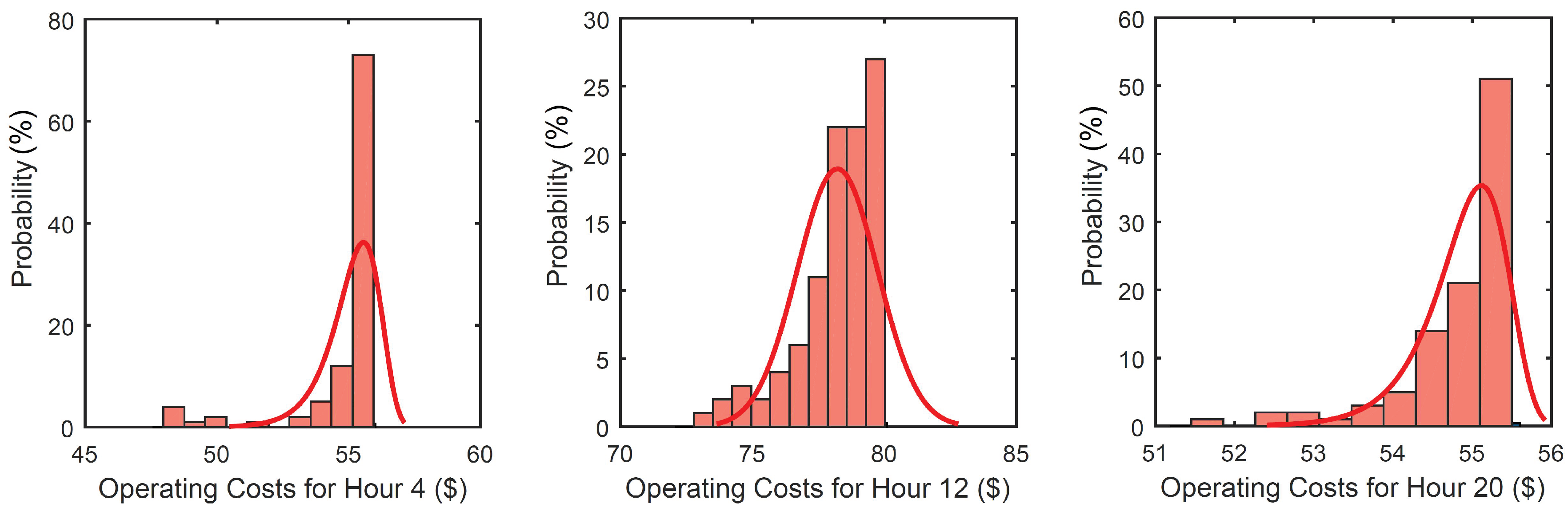
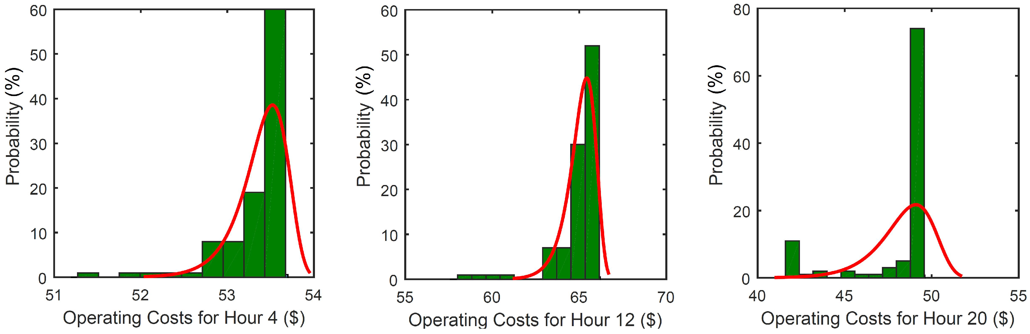
For each hourly operating cost, a probability-normalized histogram is constructed to assess the influence of uncertainties. The operating costs for the three representative hours (4th hour, 12th hour, and 20th hour) in four example days are shown in Figure 9, Figure 10, Figure 11 and Figure 12, respectively. The probability-normalized histograms show the potential operating costs and their probabilities in different price ranges. In other words, the distribution illustrates how probable each operating cost is for the given operating conditions.

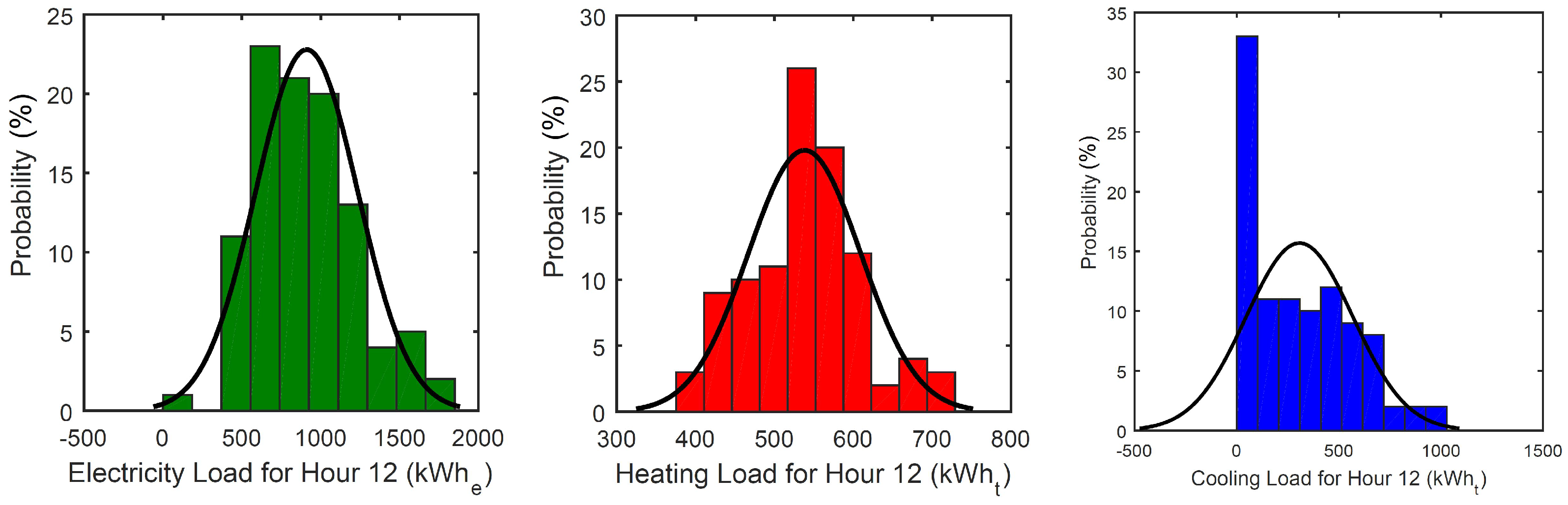
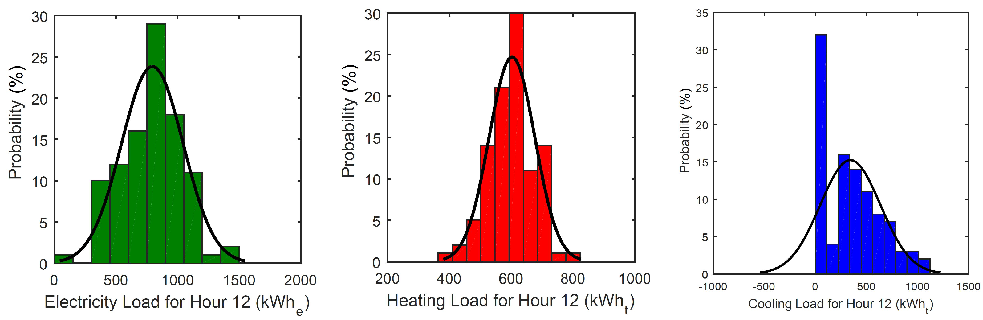
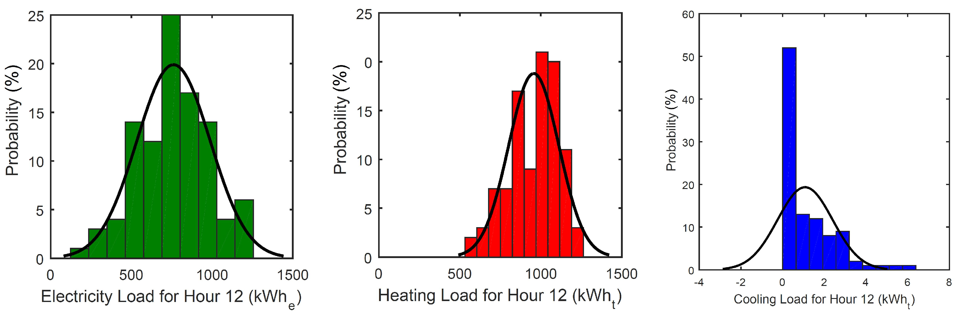
The uncertainties of solar PV and wind power generation drive the uncertainty in power generation overall when using renewable energy resources (Figure 13, Figure 14, Figure 15 and Figure 16). It is important to note that the probability of zero power generation is also included in the plots, which can affect the general distributions. The solar irradiation values are drawn from a normal distribution while the wind speeds are from a Weibull distribution. Consequently, the potential operating costs have various distributions at different hours during the day. For instance, the operating cost follows a normal distribution during hours when the the majority of power generation comes from solar PV panels. Similarly, when wind generation dominates the makeup of electric power provided, the operating cost reflects a Weibull distribution. On the other hand, the effects from other systems are not as pronounced since energy systems such as the CHP generation, the electrical grid, and natural gas boilers are assumed to be readily available when needed. Statistical distributions of all considered power generation methods influence the type of distribution of the operating cost; however, the operating cost probability distribution tends to take the shape of the probability distribution for the source with the most uncertainty. Furthermore, the statistical distributions of energy loads are represented by normal distributions (Figure 17, Figure 18, Figure 19 and Figure 20). The expected energy loads have Gaussian curves that center about their mean values. Therefore, the effect on the operating cost from the expected energy loads are determined by the means and standard deviations of the energy loads. For instance, the high variance (and, therefore, large standard deviation) of the cooling load during early afternoon hours leads to unpredictable cooling demand in those hours.

The addition of heating and cooling loads in the analysis of the DES has generated considerable differences compared to studies of DES without heating and cooling loads. As mentioned in the proposed DES section, all of the cooling equipment is run by electrical power. In other words, the power generation from energy systems in the DES needs to fulfill both the electricity demand and the electrical energy required by the cooling equipment. During events of high electricity and cooling demands, it is more likely for the DES to purchase power from the grid because the on-site generation is not adequate. From Table 5, the standard deviation of the operating cost often exceeds $2 during peak energy demand, which typically occurs around 12 p.m. and in the early afternoon. This observation indicates that the uncertainty of the operating cost of the DES increases during events of high energy consumption. This is due to the presence of uncertainties from electricity, heating, and cooling demands. It is also notable that the standard deviations of the operating costs on the last four hours on 20 March are considerably higher than the other hours. This is caused by the uncertainty of heating load during those hours.

The projected operating costs of the proposed DES on four example days are compared to the operating costs of the current energy system during the same periods (Table 6). Studies of DES without consideration of all three major energy loads do not provide a complete picture of the total energy consumption and operating cost. This study includes both electrical and thermal loads for more comprehensive results. The proposed DES with a mixed of power generation systems shows potential for operating cost reductions. The probabilistic operating cost savings are around $150/day (approximately 10%) compared to the actual operating cost. Overall, the strategic implementation of power generation from various sources reduces the overall operating cost of the DES.

Throughout this study, there are limitations on the applicability of this method that could be addressed by future studies on reducing the operating cost of DES with stochasticity in power generation and energy demands. Critical limitations are as follows:

• The performance of solar PV panels is assumed to be consistent throughout the lifetime of the renewable energy systems. In other words, the degradation of the energy system is not considered.
• The operating costs on the four example days are based on the specific system sizes that were detailed in Table 2. Design choices will influence the operating cost, but variations in the design of the various systems were not considered here.
• The CHP and boiler are assumed to be readily available. The uncertainties from these systems are not considered.
• The unit operating costs for the energy systems are consistent throughout the year. Monthly and seasonal changes in unit costs will influence the operating costs throughout the year.
• The start-up and shut-down costs of the energy systems are not considered.
• All of the variables are hourly. Fluctuations in power generation and energy loads on a sub-hourly basis are not accounted for here.
• The examples days do not capture extreme conditions/design days. Instead, the beginning days of four different astronomical seasons are studied, capturing a variety of conditions outside of the summer and winter design days.

4. Conclusions

DES optimization for a district of metered buildings has been investigated in this paper with consideration of uncertainties in energy loads and power generation of renewable energy resources. The optimization of this DES minimizes the operating cost, which includes the cost of meeting the electricity, heating, and cooling loads. The simulation results suggest that the operating cost of the proposed DES is less than the operating cost of the current energy system (by approximately 10%); however, the uncertainties in the system lead to unpredictability in the operating cost. Analyses based on statistical probability were demonstrated to have the capability to predict probable operating costs at a given time period.

A Monte Carlo statistical simulation has been used to incorporate the uncertainty of energy loads and power generation from renewable power generation into the DES model. The results from the case study using four example days have shown the influence of uncertain input variables. The operating cost at each hour of the four example days is heavily dependent on the sources of power generation. Even though the uncertainties of all renewable sources of power generation add to the uncertainty in the operating cost, the most dominating source of power generation at a given period determines the distribution of the operating cost. Furthermore, the uncertainty in operating cost of the electricity load is more prominent than the uncertainty in operating cost of the heating load. This is because the use of natural gas for heating is more reliable than power generation from renewable energy resources.

The low operating costs of the energy systems used in the DES contribute toward the low overall operating cost. The proposed DES incorporates solar PV and wind turbines for power generation, which can often operate at a lower cost per unit of electricity compared to purchased electricity from the grid. With on-site generation, the purchased power from the electrical grid on the four example days can be reduced by up to 26%. It is important to recognize that the percentage of on-site power generation (i.e., the reduction in purchased power) on different days of the year can vary from the on-site power generation of the four example days. Nonetheless, the buildings can be less dependent on the grid and the overall operating cost can be lowered.

In conclusion, a DES incorporating renewable energy systems offers operating cost reduction opportunities. However, the uncertainties associated with renewable energy resources can cause unreliable power generation, leading to uncertainty in operating costs. Additionally, consideration of uncertainties in the energy loads is also important. The addition of uncertainties from the electricity, heating, and cooling loads can further contribute to unpredictable operating costs. Even though the energy loads exhibit normal distributions, those with high variance can increase (or decrease) the required loads to be fulfilled. Thus, the operating cost can be highly unpredictable. A statistical analysis that incorporates the expected uncertainty is recommended for DES planning with renewable energy resources, as a deterministic calculation may give a misleading picture of the likely operating costs and potential savings.

References

- Thornton, A.; Monroy, C.R. Distributed power generation in the United States. Renew. Sustain. Energy Rev. 2011, 15, 4809–4817. [Google Scholar] [CrossRef]
- Ehsan, A.; Yang, Q. Optimal integration and planning of renewable distributed generation in the power distribution networks: A review of analytical techniques. Appl. Energy 2018, 210, 44–59. [Google Scholar] [CrossRef]
- Mokgonyana, L.; Zhang, J.; Li, H.; Hu, Y. Optimal location and capacity planning for distributed generation with independent power production and self-generation. Appl. Energy 2017, 188, 140–150. [Google Scholar] [CrossRef]
- Bilgili, M.; Ozbek, A.; Sahin, B.; Kahraman, A. An overview of renewable electric power capacity and progress in new technologies in the world. Renew. Sustain. Energy Rev. 2015, 49, 323–334. [Google Scholar] [CrossRef]
- Van der Walt, H.L.; Bansal, R.C.; Naidoo, R. PV based distributed generation power system protection: A review. Renew. Energy Focus 2018, 24, 33–40. [Google Scholar] [CrossRef]
- Tran, T.T.; Smith, A.D. Evaluation of renewable energy technologies and their potential for technical integration and cost-effective use within the U.S. energy sector. Renew. Sustain. Energy Rev. 2017, 80, 1372–1388. [Google Scholar] [CrossRef]
- Lorenzo, B.; Stefano, C.; Vincenzo, M.; Vittorio, R.; Luis, R.J. Hybrid renewable energy systems for renewable integration in microgrids: Influence of sizing on performance. Energy 2018, 152, e7–e133. [Google Scholar] [CrossRef]
- Domenech, B.; Ranaboldo, M.; Ferrer-Martí, L.; Pastor, R.; Flynn, D. Local and regional microgrid models to optimise the design of isolated electrification projects. Renew. Energy 2018, 119, 795–808. [Google Scholar] [CrossRef]
- Zachar, M.; Daoutidis, P. Understanding and predicting the impact of location and load on microgrid design. Energy 2015, 90, 1005–1023. [Google Scholar] [CrossRef]
- Jacob, A.S.; Banerjee, R.; Ghosh, P.C. Sizing of hybrid energy storage system for a PV based microgrid through design space approach. Appl. Energy 2018, 212, 640–653. [Google Scholar] [CrossRef]
- Mazzola, S.; Astolfi, M.; Macchi, E. The potential role of solid biomass for rural electrification: A techno economic analysis for a hybrid microgrid in India. Appl. Energy 2016, 169, 370–383. [Google Scholar] [CrossRef]
- Aluisio, B.; Dicorato, M.; Forte, G.; Trovato, M. An optimization procedure for Microgrid day-ahead operation in the presence of CHP facilities. Sustain. Energy Grids Netw. 2017, 11, 34–45. [Google Scholar] [CrossRef]
- Lupangu, C.; Bansal, R.C. A review of technical issues on the development of solar photovoltaic systems. Renew. Sustain. Energy Rev. 2017, 73, 950–965. [Google Scholar] [CrossRef]
- Pazouki, S.; Haghifam, M.R.; Moser, A. Electrical Power and Energy Systems Uncertainty modeling in optimal operation of energy hub in presence of wind, storage and demand response. Int. J. Electr. Power Energy Syst. 2014, 61, 335–345. [Google Scholar] [CrossRef]
- Soroudi, A.; Amraee, T. Decision making under uncertainty in energy systems: State of the art. Renew. Sustain. Energy Rev. 2013, 28, 376–384. [Google Scholar] [CrossRef]
- Parisio, A.; Del Vecchio, C.; Vaccaro, A. A robust optimization approach to energy hub management. Int. J. Electr. Power Energy Syst. 2012, 42, 98–104. [Google Scholar] [CrossRef]
- Evins, R.; Orehounig, K.; Dorer, V.; Carmeliet, J. New formulations of the ’energy hub’ model to address operational constraints. Energy 2014, 73, 387–398. [Google Scholar] [CrossRef]
- Mavromatidis, G.; Orehounig, K.; Carmeliet, J. Design of distributed energy systems under uncertainty: A two-stage stochastic programming approach. Appl. Energy 2018. [Google Scholar] [CrossRef]
- Jabbari-Sabet, R.; Moghaddas-Tafreshi, S.M.; Mirhoseini, S.S. Microgrid operation and management using probabilistic reconfiguration and unit commitment. Int. J. Electr. Power Energy Syst. 2016, 75, 328–336. [Google Scholar] [CrossRef]
- Fioriti, D.; Giglioli, R.; Poli, D. Short-term operation of a hybrid minigrid under load and renewable production uncertainty. In Proceedings of the 2016 IEEE Global Humanitarian Technology Conference (GHTC), Seattle, WA, USA, 13–16 October 2016; pp. 436–443. [Google Scholar]
- Mavromatidis, G.; Orehounig, K.; Carmeliet, J. A review of uncertainty characterisation approaches for the optimal design of distributed energy systems. Renew. Sustain. Energy Rev. 2018, 88, 258–277. [Google Scholar] [CrossRef]
- Olsthoorn, D.; Haghighat, F.; Mirzaei, P.A. Integration of storage and renewable energy into district heating systems: A review of modelling and optimization. Solar Energy 2016, 136, 49–64. [Google Scholar] [CrossRef]
- Li, Y.; Rezgui, Y.; Zhu, H. District heating and cooling optimization and enhancement—Towards integration of renewables, storage and smart grid. Renew. Sustain. Energy Rev. 2017, 72, 281–294. [Google Scholar] [CrossRef]
- Najibi, F.; Niknam, T. Stochastic scheduling of renewable micro-grids considering photovoltaic source uncertainties. Energy Convers. Manag. 2015, 98, 484–499. [Google Scholar] [CrossRef]
- Nikmehr, N.; Najafi-Ravadanegh, S.; Khodaei, A. Probabilistic optimal scheduling of networked microgrids considering time-based demand response programs under uncertainty. Appl. Energy 2017, 198, 267–279. [Google Scholar] [CrossRef]
- Yılmaz Balaman, S.; Selim, H. Sustainable design of renewable energy supply chains integrated with district heating systems: A fuzzy optimization approach. J. Clean. Prod. 2016, 133, 863–885. [Google Scholar] [CrossRef]
- Lu, S.; Gu, W.; Zhou, J.; Zhang, X.; Wu, C. Coordinated dispatch of Multi-Energy System with District Heating Network: Modeling and Solution Strategy. Energy 2018, 152, 358–370. [Google Scholar] [CrossRef]
- Sameti, M.; Haghighat, F. Optimization approaches in district heating and cooling thermal network. Energy Build. 2017, 140, 121–130. [Google Scholar] [CrossRef]
- Gang, W.; Augenbroe, G.; Wang, S.; Fan, C.; Xiao, F. An uncertainty-based design optimization method for district cooling systems. Energy 2016, 102, 516–527. [Google Scholar] [CrossRef]
- Li, C.Z.; Shi, Y.M.; Liu, S.; Zheng, Z.L.; Liu, Y.C. Uncertain programming of building cooling heating and power (BCHP) system based on Monte-Carlo method. Energy Build. 2010, 42, 1369–1375. [Google Scholar] [CrossRef]
- Mavromatidis, G.; Orehounig, K.; Carmeliet, J. Uncertainty and global sensitivity analysis for the optimal design of distributed energy systems. Appl. Energy 2018, 214, 219–238. [Google Scholar] [CrossRef]
- Dantzig, G.B. Linear Programming under Uncertainty. Manag. Sci. 1955, 1, 197–206. [Google Scholar] [CrossRef]
- SkyFoundry. SkySpark-SkyFoundry. Available online: https://skyfoundry.com/ (accessed on 23 January 2019).
- ASHRAE. American Society of Heating, Refrigerating and Air-Conditioning Engineers. Available online: https://www.ashrae.org/ (accessed on 23 January 2019).
- National Renewable Energy Laboratory (NREL). Wind Data. Available online: https://www.nrel.gov/gis/data-wind.html (accessed on 23 January 2019).
- National Renewable Energy Laboratory (NREL). Advancing the Science of Solar Data; NREL: Golden, CO, USA, 2018.
- National Renewable Energy Laboratory. Distributed Generation Renewable Energy Estimate of Costs; Technical Report; NREL: Golden, CO, USA, 2016.
- US Environmental Protection Agency. Catalog of CHP Technologies; US Environmental Protection Agency: Washington, DC, USA, 2015.
- US Environmental Protection Agency. Fact Sheet: CHP as a Boiler Replacement Opportunity; US Environmental Protection Agency: Washington, DC, USA, 2013; pp. 1–6.
- Wais, P. A review of Weibull functions in wind sector. Renew. Sustain. Energy Rev. 2017, 70, 1099–1107. [Google Scholar] [CrossRef]
- Harris, R.I.; Cook, N.J. The parent wind speed distribution: Why Weibull? J. Wind Eng. Ind. Aerodyn. 2014, 131, 72–87. [Google Scholar] [CrossRef]
- Sedić, A.; Pavković, D.; Firak, M. A methodology for normal distribution-based statistical characterization of long-term insolation by means of historical data. Sol. Energy 2015, 122, 440–454. [Google Scholar] [CrossRef]
- Tran, T.T.; Smith, A.D. Incorporating performance-based global sensitivity and uncertainty analysis into LCOE calculations for emerging renewable energy technologies. Appl. Energy 2018, 216, 157–171. [Google Scholar] [CrossRef]
- Kennedy, J.; Eberhart, R.C. Particle Swarm Optimization. In Proceedings of the IEEE International Conference on Neural Networks, Perth, Australia, 27 November–1 December 1995; pp. 1942–1948. [Google Scholar]
- Kulkarni, N.K.; Patekar, S.; Bhoskar, T.; Kulkarni, O.; Kakandikar, G.M.; Nandedkar, V.M. Particle Swarm Optimization Applications to Mechanical Engineering—A Review. Mater. Today Proc. 2015, 2, 2631–2639. [Google Scholar] [CrossRef]
- Mazhoud, I.; Hadj-Hamou, K.; Bigeon, J.; Joyeux, P. Particle swarm optimization for solving engineering problems: A new constraint-handling mechanism. Eng. Appl. Artif. Intell. 2013, 26, 1263–1273. [Google Scholar] [CrossRef]
- Marini, F.; Walczak, B. Particle swarm optimization (PSO). A tutorial. Chemom. Intell. Lab. Syst. 2015, 149, 153–165. [Google Scholar] [CrossRef]
Figure 1.
Daily energy loads on 21 June and its neighboring days.
Figure 2.
Average electricity load of the districts of buildings.
Figure 3.
Average heating load of the districts of buildings.
Figure 4.
Average cooling load of the districts of buildings.
Figure 5.
Diagram of the proposed district energy system management.
Figure 6.
Average wind speed and solar irradiation at the study location (Salt Lake City).
Figure 7.
Flowchart of the Monte Carlo simulation and the Particle Swarm Optimization algorithm.
Figure 8.
Operating costs of the DES of the four example days.
Figure 9.
Probability of the operating cost on the 4th hour (left), 12th hour (center), and 20th hour (right) of the 20 March case study.
Figure 10.
Probability of the operating cost on the 4th hour (left), 12th hour (center), and 20th hour (right) of the 21 June case study.
Figure 11.
Probability of the operating cost on the 4th hour (left), 12th hour (center), and 20th hour (right) of the 22 September case study.
Figure 12.
Probability of the operating cost on the 4th hour (left), 12th hour (center), and 20th hour (right) of the 21 December case study.
Figure 13.
Probability of the power generation from solar PV (left) and wind (right) at the 12th hour on the 20 March case study.
Figure 14.
Probability of the power generation from solar PV (left) and wind (right) at the 12th hour on the 21 June case study.
Figure 15.
Probability of the power generation from solar PV (left) and wind (right) at the 12th hour on the 22 September case study.
Figure 16.
Probability of the power generation from solar PV (left) and wind (right) at the 12th hour on the 21 December case study.
Figure 17.
Probability of electricity load (left), heating (center), and cooling load (right) of the 12th hour on 20 March.
Figure 18.
Probability of electricity load (left), heating (center), and cooling load (right) of the 12th hour on 21 June.
Figure 19.
Probability of electricity load (left), heating (center), and cooling load (right) of the 12th hour on 22 September.
Figure 20.
Probability of electricity load (left), heating (center), and cooling load (right) of the 12th hour on 21 December.