Article

Fast Processing Intelligent Wind Farm Controller for Production Maximisation

1
US Pakistan Center for Advanced Studies in Energy, University of Engineering and Technology (UET), Peshawar 25000, Pakistan
2
School of Engineering, Durham University, Durham DH1 3LE, UK
3
Engie Green, 59777 Lille, France
*
Author to whom correspondence should be addressed.
Energies 2019, 12(3), 544; https://doi.org/10.3390/en12030544
Submission received: 26 December 2018 / Revised: 2 February 2019 / Accepted: 6 February 2019 / Published: 10 February 2019
(This article belongs to the Special Issue State of the Art of Wind Farm Optimization)

Abstract

:
A practical wind farm controller for production maximisation based on coordinated control is presented. The farm controller emphasises computational efficiency without compromising accuracy. The controller combines particle swarm optimisation (PSO) with a turbulence intensity–based Jensen wake model (TI–JM) for exploiting the benefits of either curtailing upstream turbines using coefficient of power ( C P ) or deflecting wakes by applying yaw-offsets for maximising net farm production. Firstly, TI–JM is evaluated using convention control benchmarking WindPRO and real time SCADA data from three operating wind farms. Then the optimised strategies are evaluated using simulations based on TI–JM and PSO. The innovative control strategies can optimise a medium size wind farm, Lillgrund consisting of 48 wind turbines, requiring less than 50 s for a single simulation, increasing farm efficiency up to a maximum of 6% in full wake conditions.

1. Introduction

Wind farms take advantages of economies of scale for reducing levelised cost of energy by clustering turbines together. However, turbines in this cluster interact with each other aerodynamically through wake effects. Wake effects, or simply wakes, can significantly impact economic performance of a wind farm by decreasing net production or increasing fatigue loads [1,2,3].
Industry best practice is to install the turbines with increased spacing in the prevailing wind directions (downwind) as compared to non-prevailing wind directions (crosswind) [2]. Wake losses in the crosswind directions can be as high as 50% due to close spacing [4], reducing wind farm efficiency to as low as 40% [5].
Another way of reducing wake effects is global optimisation of the whole wind farm using coordinated control. With state of the art (greedy control), every turbine maximises its own production, neglecting the wake effects on shadowed turbines [2]. Coordinated control based on global optimisation of the whole wind farm, instead of local optimisation of individual turbines, can result in increased annual energy production [6].
Coordinated control is the farm level control (termed “farm control” or “optimised control as well”), which is based on the optimised cooperation or coordination of turbines in the farm. In such control setups, turbines coordinate with each other to increase the net production. Curtailing or yawing the upstream turbines reduces the wake effects produced, hence increasing production of the downstream turbines. Net gain in farm production can be achieved if the decrease in curtailed turbines’ production is compensated by an increase in shadowed turbines’ production.
A review of coordinated control studies in [7,8] concludes that the realisation of benefits of coordinated control depends upon terrain characteristics, atmospheric wind conditions, layout of the wind farm and number of turbines under consideration. Wakes recover quickly in rough terrains as compared to smooth surfaces (offshore) [7]. In certain wind directions, downstream turbines are under significant wake effects, impacting their production negatively. Usually negligible wake effects are observed at higher wind speeds in above-rated wind conditions [5]. Net production of denser wind farms (with closely spaced turbines) is generally affected more by wake effects [5].
Coordinated control can be performed with optimal settings of C P or yaw-offsets ( α ) of the upstream turbines. The only change required in the existing control system will be the coordinated control algorithm, specifically a change in the software [4,9]. Intelligent farm control aimed at maximising net present value will replace turbine power curve as the main performance characteristic [6]. Real time online coordinated control requires the optimisation process to be completed in the order of seconds [6,10]. This paper aims to develop online, accurate and computationally efficient coordinated control strategies for production maximisation. Particle swarm optimisation PSO is combined with a fast processing wind deficit model, the turbulence intensity–based Jensen wake model (TI–JM), for developing a realistic and practical online wind farm controller. A field implementation of coordinated control strategies based on this work is presented in [8].
This paper is structured in different sections, described as follows. Different wind and wake modelling techniques are briefly explained in Section 2. A brief overview of TI–JM is given in Section 3. This is followed by detailing the optimisation process in Section 4 with the control problem and objective function formulation in Section 4.1 and details of PSO in Section 4.2. Information about the three wind farms: Brazos, Le Sole de Moulin Vieux (SMV) and Lillgrund is provided in Section 5.1, Section 5.2 and Section 5.3 respectively. The methodologies for obtaining efficiencies of the farms case studies are discussed in Section 6. Results and analyses are presented in Section 7. Conclusion of this work is given in Section 8.

2. Wind and Wake Modeling

A brief overview of different wake models available in literature is presented in this section. Wake models can generally be divided into two categories; complex computational fluid dynamics (CFD) models and simplified engineering models [11,12,13,14,15,16,17]. Wind is a complex fluid as a number of parameters affect the wind flow, such as boundary layer conditions, wind shear, turbulence intensity, and terrain characteristics [18]. Complex fluids can be considered homogeneous at the macroscopic (or bulk) scale, but are disordered at the “microscopic” scale, and possess structure at an intermediate scale [18]. The key elements of CFD modelling are the grid or mesh generation, algorithm development and turbulence modelling. The higher the resolution of the mesh, the higher will be the accuracy and computational requirements for the model. Complexity of a CFD model depends upon the way turbulence is modeled and solved [19]. Eddy viscosity [20], large eddy simulation [21], and k ϵ [22] are some of the examples of CFD models. These CFD models can provide detailed information about wind flow. However the computational requirements required for wake modelling are extremely high. For example, the CFD model used in [16] for simulating a single wake between two turbines take 30 h for processing using a 256 cores. This makes CFD models unsuitable for real time online coordinated control.
Engineering wake models use empirical or analytical expressions for predicting wind deficit in a wind farm. This makes them computationally efficient but relatively less accurate as compared to CFD models. These models contain simple models for turbulence and surface roughness and can provide quick and accurate solutions for mean wind flows [23]. Engineering models are useful for predicting mean wind deficit inside the wind farm and for estimating wind farm efficiency, but they do not provide details of the wake flow process [20]. These models can be easily executed on a standard personal computer. Despite their simplicity, engineering models can be highly effective for predicting power production if the parameters are tuned well [24]. The Jensen model [25,26], Larsen model [27] and Frandsen model [28] are examples of engineering wake flow models.
If detailed wake flow information is not required then it is better to combine the accuracy of CFD models with the computational efficiency of engineering models [4,29]. The parameters such as wake decay coefficients and wake expansion factors in engineering models shall be tuned with reference to wind farm data or a higher order CFD model, as suggested in [4,13,14,24,29,30,31,32,33,34,35,36,37]. This can be achieved by combining analytical expressions based on CFD models with engineering models. A comparative analysis of different CFD and engineering wake models in [2,7,16] concludes that the Jensen model is the most suitable for feedback control systems, due to its computational efficiency. However, the parameters must be tuned according to the wind conditions and terrain on site [4,29,31,33,35,38]. The wind deficit model developed and used in this paper, named TI–JM, is based on this principal explained in the next section.

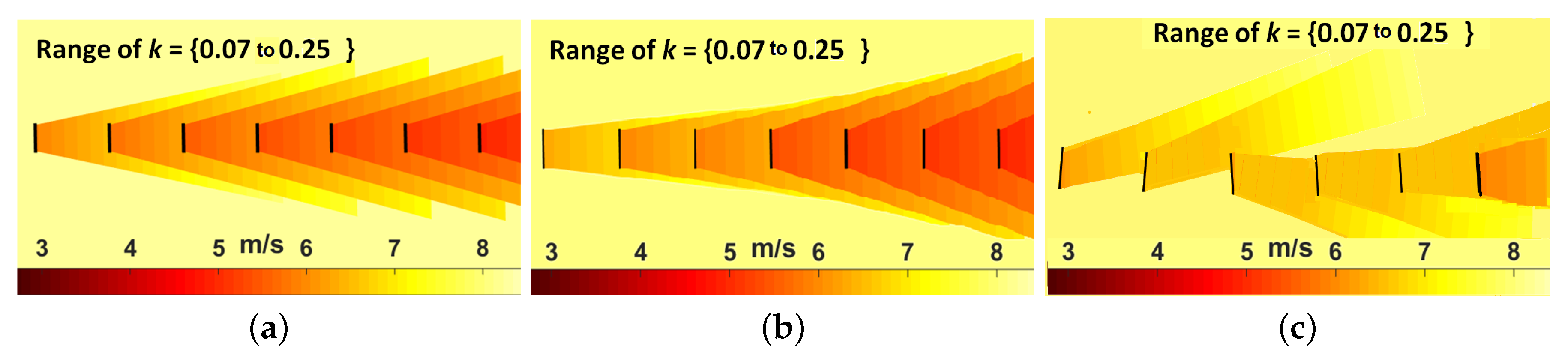
3. Turbulence Intensity–Based Jensen Model (TI–JM)

This section gives a brief overview of TI–JM, which is used for developing the coordinated control strategies. The detailed methodology for developing TI–JM and validation using real-time data is given in [7]. TI–JM modifies the wake decay coefficient (k) of the standard Jensen model [25,26] using wake-added turbulence intensity. Wake decay coefficient presents how quickly the wake diffuses depending on hub height of the wake generating turbine (z) and the surface roughness length ( z 0 ) as given in Equation (1) [25,26]. TI–JM has all the characteristics of the standard Jensen model [25,26] except for the constant k.
k = 1 / [ 2 ln ( z / z 0 ) ]
The Jensen model has widely been used for developing farm control strategies due to its processing efficiency [2,4,7,8,39,40,41,42] and is also part of many industry standard software such as WindFarmer [7] and WindPRO [31]. Simple assumptions such as the ideal wind flow, constant k and linear wake expansion make the Jensen model computationally very efficient. However, keeping k constant means ignoring the farm-added roughness and wake-added turbulence intensity, making the model less accurate [4,29].
Wake affected turbines experience more turbulent wind as the farm acts as a roughness generator itself, because of the additional turbulence intensity [29,31]. This wake-added turbulence intensity must be considered for estimating wind speed deep inside a wind farm. TI–JM follows this principle and uses the wake added turbulence intensity along with free-stream turbulence intensity for estimating k and wind deficit inside the wind farm using Equation (2) [43]. Turbulence intensity is composed of lateral, vertical and longitudinal components. The longitudinal component ( I L ) can be determined using Equation (2) [43]. The wind speed deficit can now be found using Equation (3) [25,26].
I L = 1 ln ( z / z 0 ) = 2 k k = I L / 2
u x = u 0 1 1 1 C T 1 + k × x r 0 2 ,
where u x denotes the wind speed at distance x from the wake producing turbine, u 0 is the wind speed at the corresponding upstream turbine, r 0 is the radius of turbine swept area and C T is the coefficient of thrust. TI–JM provides speedy and accurate results, requiring minimum parameters as inputs, which are generally easily available from Supervisory Control And Data Acquisition (SCADA) data. If a turbine is affected by multiple or overlapping wakes then these are superimposed by taking a a linear superposition of the squared deficits (based on kinetic energy deficits), is used for this purpose, as suggested in [26].

4. Optimisation

In order to use the controller online, an acceptable solution has to be achieved in the order of seconds so that the C P or yaw-offset of each turbine can be calculated before the wind reaches it, as communicating these optimised values will also take some time.
Previous research on wind farm coordinated control emphasises more on the aerodynamics of the problem, providing little or no information of the optimisation process. Wind farm coordinated control is a complex optimisation problem as each individual turbine’s production is a dimension of the farm production [40]. Numerical optimisation [1,10,44,45,46,47,48,49,50,51], game-theoretic approach [39,42,52], hill climbing algorithm [53] and genetic algorithm [41,54] are some of the techniques used for solving the coordinated control problem. However, It is suggested in [3,9] that iterative algorithms can improve performance of farm controllers. Therefore, performance of different optimisation techniques (brute force, genetic algorithm, simulated annealing and PSO) were evaluated for wind farm coordinated control in [40], concluding that PSO can solve the coordinated control problem with high accuracy, speed and success rate as compared to other evaluated techniques. Details of PSO for optimising wind farm power production using coordinated control are given in Section 4.2.

4.1. Objective Function

Net production of a wind farm is the sum of individual wind turbines’ productions as given in Equation (4) [2],
P Wakes = i = 1 N P T ( i ) = i = 1 N 1 2 ρ A u ( i ) 3 C P ( i ) cos 2 α i ,
where ( P Wakes ) is the total farm production, (N) shows the total number of turbines in the wind farm, ( P T ( i ) ) is the power production of i-th turbine under consideration, air density is given by ( ρ ), turbine swept area is (A) and ( α ) is the yaw-offset.
Usually ρ remains constant inside the wind farm. If it is assumed that turbines in the farm have same configuration then the term ( 1 2 ρ A ) is constant. Ignoring this constant term means that the objective function or control problem is to maximise i = 1 N u ( i ) 3 C P ( i ) cos 2 α i in Equation (4).
The term ( cos 2 α ) quantifies the impact of yaw-offset on a turbine’s power production. Different exponents of cos α (in Equation (4)) have been used in literature [7]. The exponent of cos α can fall in the range of 1 to 5 depending on the turbines and farm under consideration [7,55,56,57,58,59]. It is discussed in [60] that there is no physical background for the exponent of cos α in Equation (4) and it can be tuned for the best-fit according to the data [61]. Different exponents of cos α were evaluated in [7] and it was observed that an exponent of “2” fits well with the given data, hence an exponent of “2” for cos α is used in this paper.
In no-wake conditions, all the turbines experience free-steam wind speed ( u 0 ) and there is no need to yaw i.e., α = 0 ° . In this case, turbines operate with maximum C P denoted by ( C P ( m a x ) ) for the specific wind speed (measured by the anemometer) according to turbine power curve. The aim is to get as close as possible to this maximum production in wake-affected wind conditions. In terms of a minimising objective function the aim is to minimise the difference between power production in no-wake conditions and power production in wake-affected conditions (actual production) as shown in Equation (5). As the constant ( 1 2 ρ A ) is ignored, the objective function ( O F ) is formulated as Equation (5):
O F = min i = 1 N u 0 3 C P ( m a x ) i = 1 N u ( i ) 3 C P ( i ) cos 2 α ( i ) .
The controller minimises the value in Equation (5) by optimally varying C P or α . When yaw-offset is applied on an upstream turbine, the wake produced deflects away from the downstream turbine’s swept area. This wake deflection is greater than the offset applied [62]. Hence wakes can be skewed away from the downstream turbine’s swept area using an optimum α . Wind deficit inside the wind farm is obtained using TI–JM. The optimisation function is linked to the TI–JM using axial induction factor, which is the loss in momentum or measure of the slowing of wind speed between free stream and the rotor plane [3,45].
The relationship between α and wake skew angle ( γ ) given in Equation (6) [62] is used in this study. This expression is developed and validated using wind tunnel experiments and real-time wind farm data [60,63,64].
γ = 1.20 × α
Equation (5) can be used for C P and yaw based optimisation. For simplicity, C P and yaw based optimisation will be studied independently: when optimising the C P settings, α will be set at zero; and conversely when optimising the turbine yaw angles, C P will be set at C P ( m a x ) for the wind speed measured by each individual turbine’s anemometer.

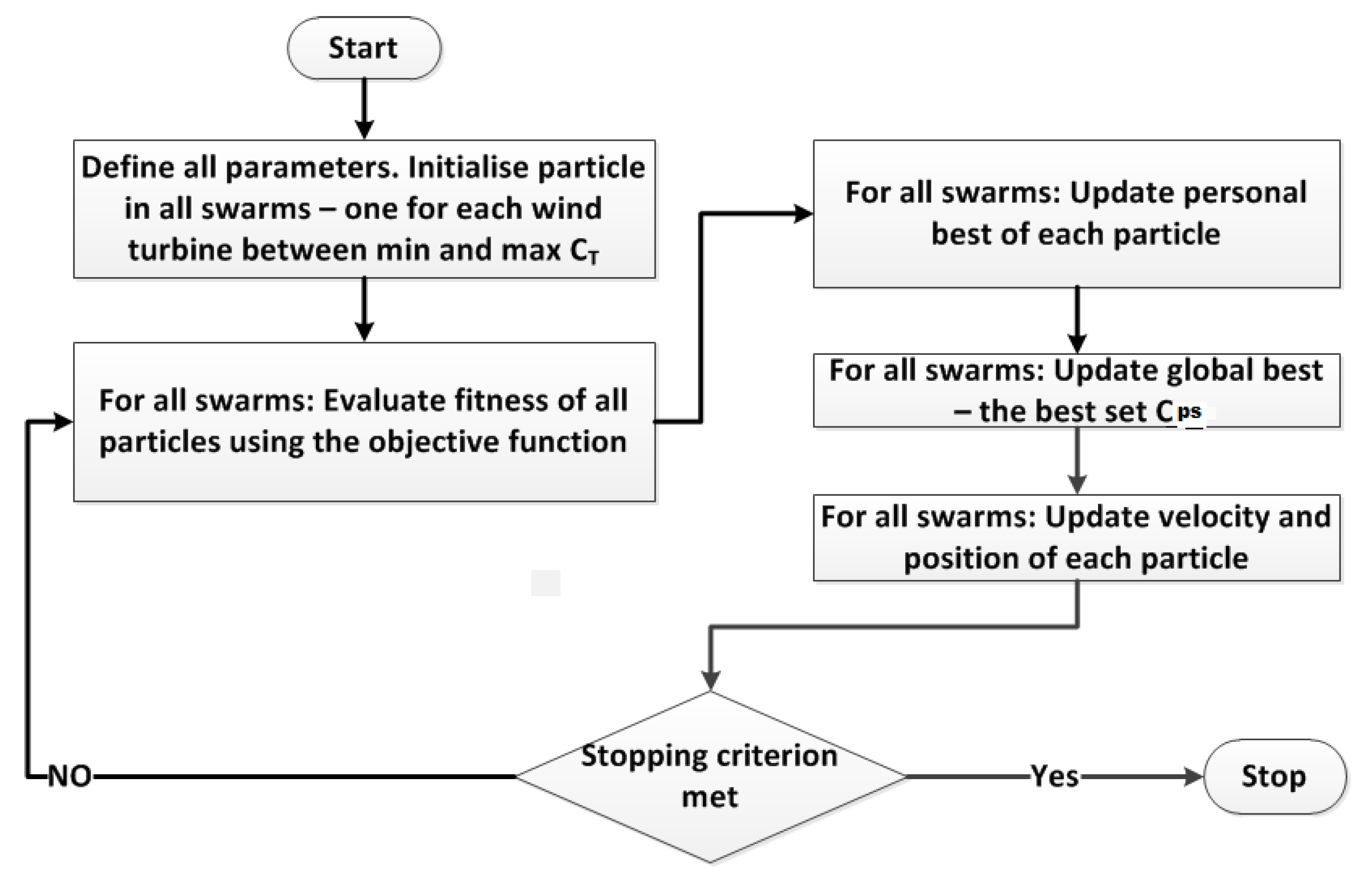
4.2. Particle Swarm Optimisation (PSO)

PSO consists of particles which move through the solution space in an organised way, by developing a collective intelligence for solving complex optimisation problems [65,66]. An individual particle represents a potential solution to the given problem. A swarm of particles represents a dimension of the objective function/control problem. Every particle’s best fitness value estimated in different iterations is recorded as the local best of that specific particle. All local bests are compared with each other and the best fitness value is recorded as the global best. Local and global bests along with the particles’ current positions are used to estimate a velocity for finding the best possible solution. The PSO version presented in [65,67] is used in this work. The optimisation process is iterative. Each iteration, the particles create a direction moving towards the global optimum with a velocity ( V i ). This V i of a given particle (i) is determined using Equation (7) [65,68]. The position ( x i ) of the particle i at time ( t + 1 ) is simply the sum of particle i’s current position at time (t) and the velocity for moving towards the next positions as given in Equation (8) [65,68].
V i ( t + 1 ) = R 1 V i ( t ) × ζ + c 1 R 2 × p i ( t ) - x i ( t ) c 2 R 3 × p g ( t ) x i ( t ) ,
x i ( t + 1 ) = x i ( t ) + V i ( t + 1 ) ,
where ( R 1 , R 2 and R 3 ) are randomness generators, inertia is denoted by ( ζ ) which controls velocity of the particles, ( c 1 , c 2 ) are constants used for controlling movement towards local and global best respectively, ( p i ) is personal best of the i-th particle in all previous t iterations, ( p g ) is the global best of the swarm and ( x i ) is current position of the i-th particle in the solution space.
The number of swarms required for optimising the objective function in Equation (5) is equal to N. Power production of each turbine is a dimension of the net farm production. The value of O F in Equation (5) is minimised in such a way, that each turbine’s optimum C P or α is achieved. Coordinated control process using C P optimisation with PSO is given in Figure 1.
The particles’ values are initialized between minimum C T and maximum C T for a given wind speed or α in a selected range ( 15 ° to 15° in this case). The optimiser then evaluates different combinations of α or C T , which is converted to C P using axial induction factor, for obtaining the power production of a given turbine. This way optimised α or C P of each individual wind turbine is calculated. TI-JM is then used to estimate the wind speed on the wake affected turbines. Sum of the power productions of all the turbines is obtained, which is subtracted from the maximum possible farm power production at that wind speed as per Equation (5). In each iteration, the farm power production obtained is compared to the previous best value. The best value for farm production among all iterations along with α or C T and C P of each turbine is recorded. These values are then communicated to each wind turbine for optimising the farm production. The algorithm terminates when all the iterations are executed.

5. Wind Farms Case Studies
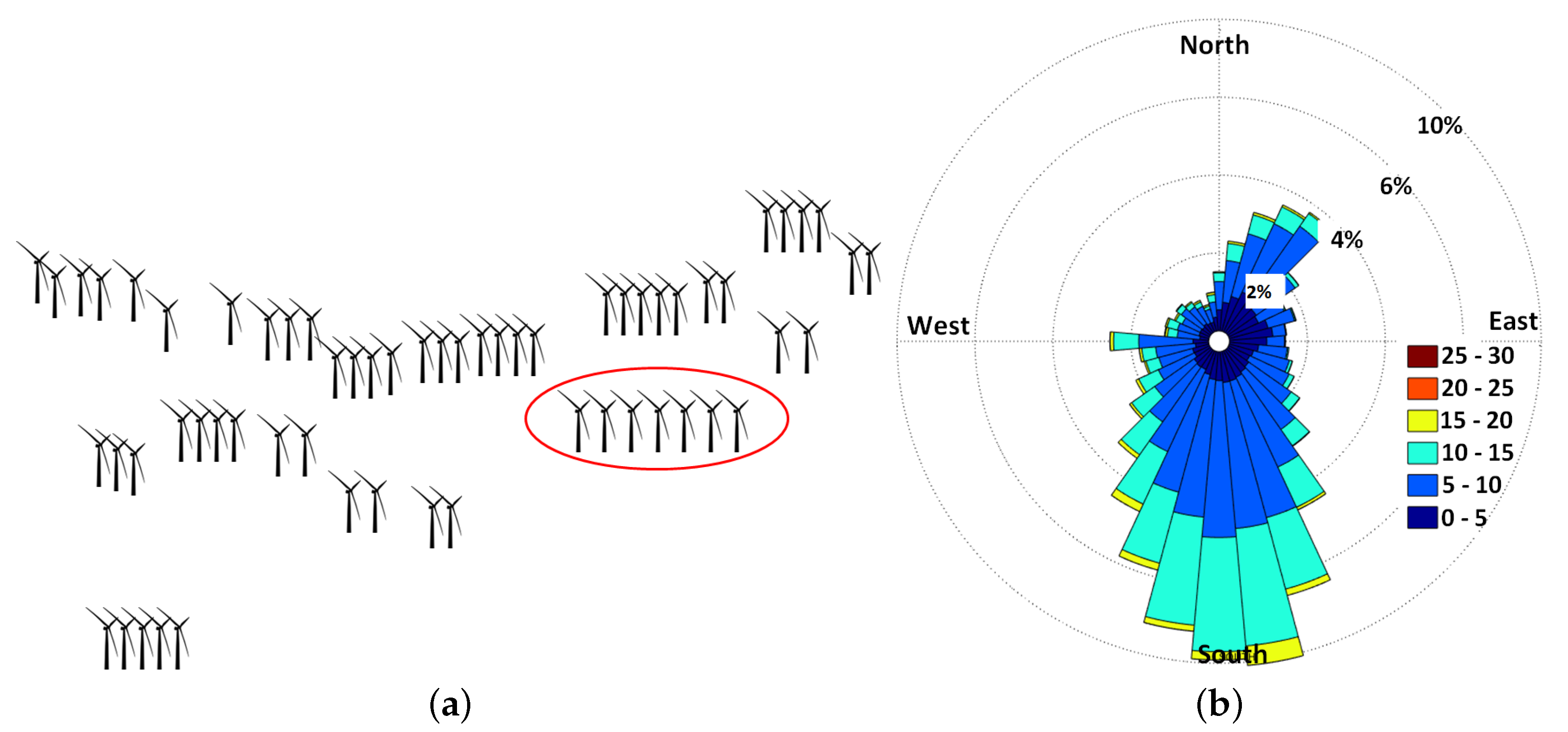
The Brazos, SMV and Lillgrund wind farms are used as case studies in this work. These three wind farms represent a diverse set in terms of layout, terrain and wind characteristics. A brief overview of these wind farms case studies is given as follows.

5.1. Brazos

Turbines in the Brazos wind farm are installed in a non-grid shape with downwind spacing up to 8 D and crosswind spacing of as low as 2 D [7]. Each row in the Brazos can be assumed to be a sub-farm for faster and efficient optimisation. The encircled row in Figure 2a is used as the case study for optimisation in this work. Seven Mitsubishi MWT 1000 turbines are installed in this row with a spacing of 3 D [7]. This case study is referred to as Brazos-row. Brazos has a flat terrain with low grass [7]. The wind–rose in Figure 2b shows the wind characteristics on site based on data from year 2004–2006.

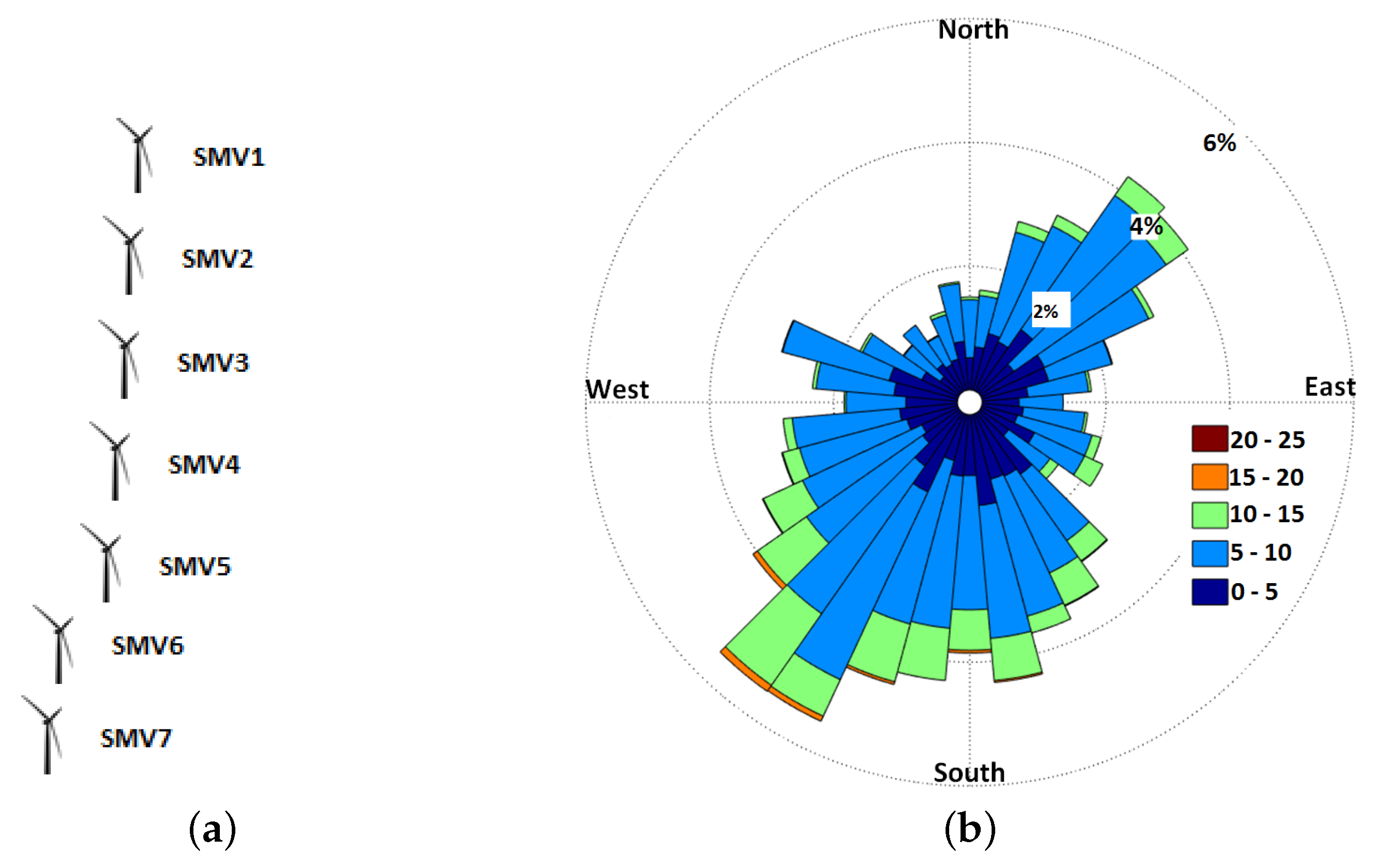
5.2. Le Sole de Moulin Vieux (SMV)
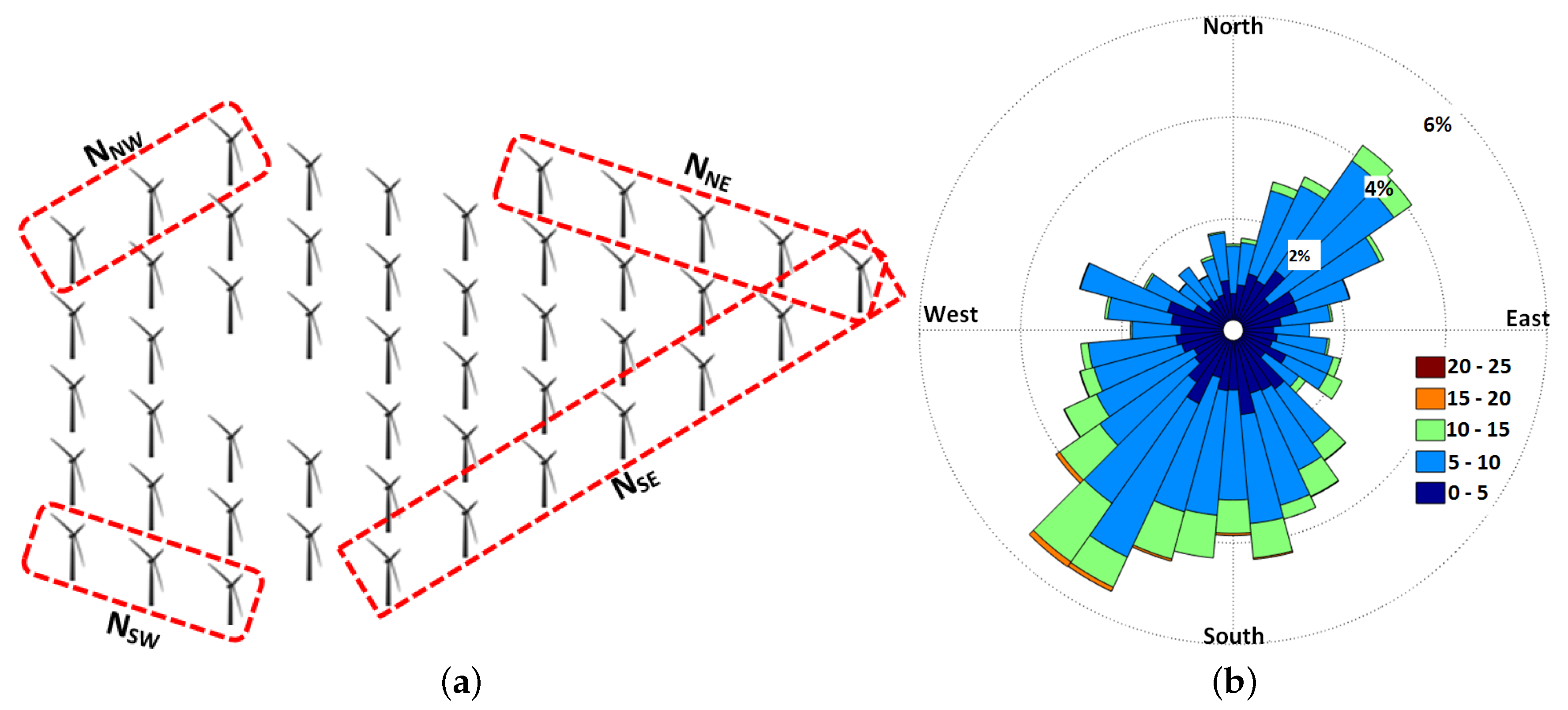
Seven Senvion MM82 2050 kW wind turbines are installed in almost like a one-dimensional array with a spacing of 3.3 D to 4.3 D as depicted in Figure 3a in the SMV wind farm. SMV has a rough terrain and vegetation is present on the ground. The farm has woods to the south at less than 1.5 D distance. These woods can cause abrupt changes in wind speed and direction [8]. Figure 3b shows wind characteristics in the farm.

5.3. Lillgrund

Lillgrund contains 48 Siemens SWT-2.3-93 turbines, installed in 8 rows as can be seen in Figure 4a. Downwind spacing is 4.5 D while crosswind spacing is 3.5 D . Lillgrund is an offshore wind farm. The wind–rose in Figure 4b shows wind characteristics in the wind farm. Wind data of 15 years (2000–2015) was used in Figure 4b using [69] at 50 m height. Performance of this wind farm is significantly affected by wakes due to the dense layout [5].

6. Methodology for Calculating Efficiency

This section details the methodology for obtaining efficiencies of the three wind farms case studies. Equation (9) [2] is used for estimating efficiencies ( η ) of Brazos-row and SMV. The denominator ( P m a x ) is simply the maximum possible farm production for a given wind speed in no-wake conditions. The numerator ( P a c t u a l ) is the actual net production of the farm.
η = P a c t u a l P m a x
Efficiency of the Lillgrund wind farm ( η L i l l ) is estimated using Equation (10) [70]:
η L i l l = N j 48 i = 1 48 P i j P j ,
where average power of the i-th turbine is denoted by ( P i ), (j) represents a set containing a specific number of turbines ( N j ) as per Table 1. The number of turbines in set j is determined using free stream wind direction. There can be four different combination in set j as it contains the turbines facing the free-stream wind, as shown in Figure 4a. Production of the j-th turbine in set j is given by ( P j ).

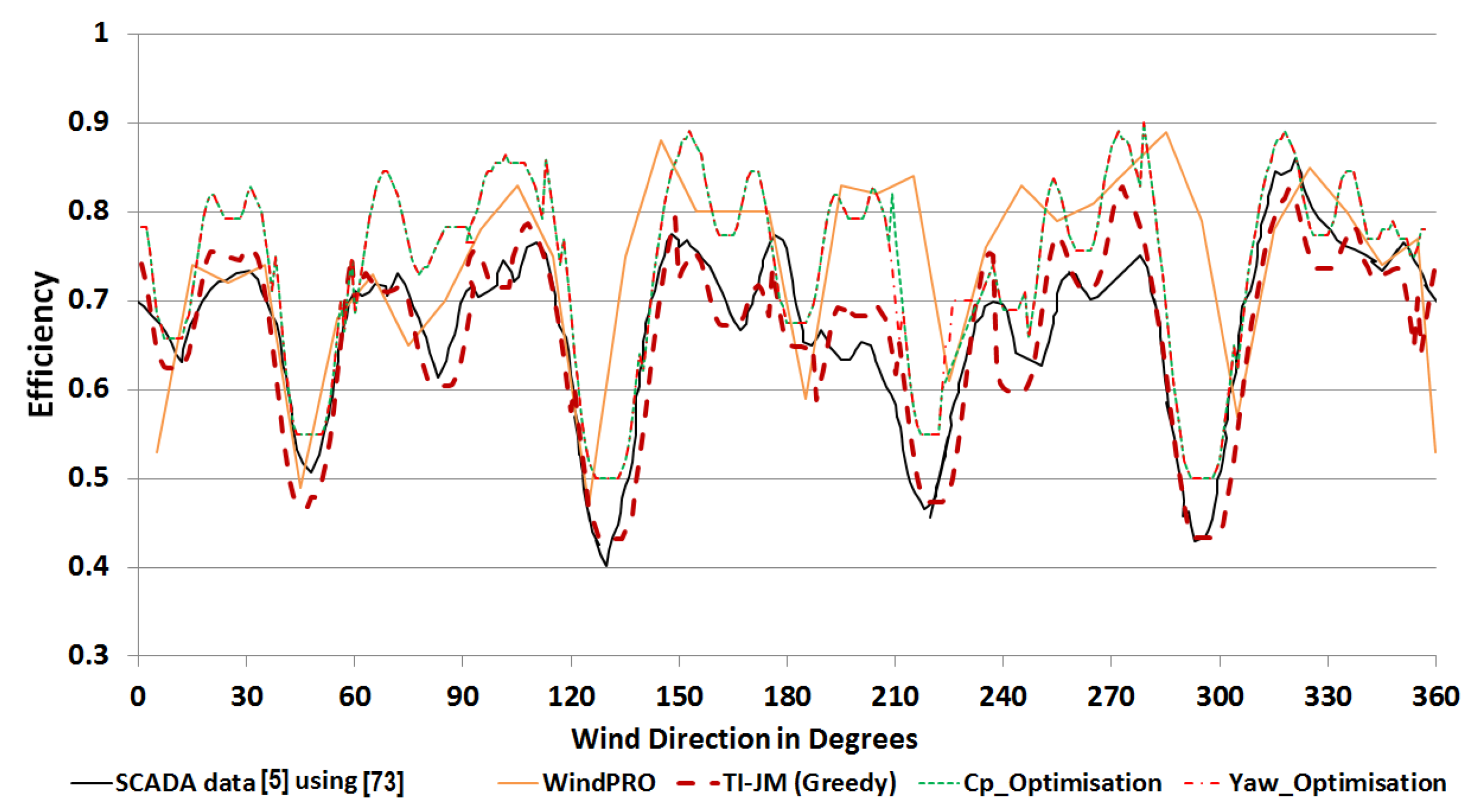
7. Results and Analyses
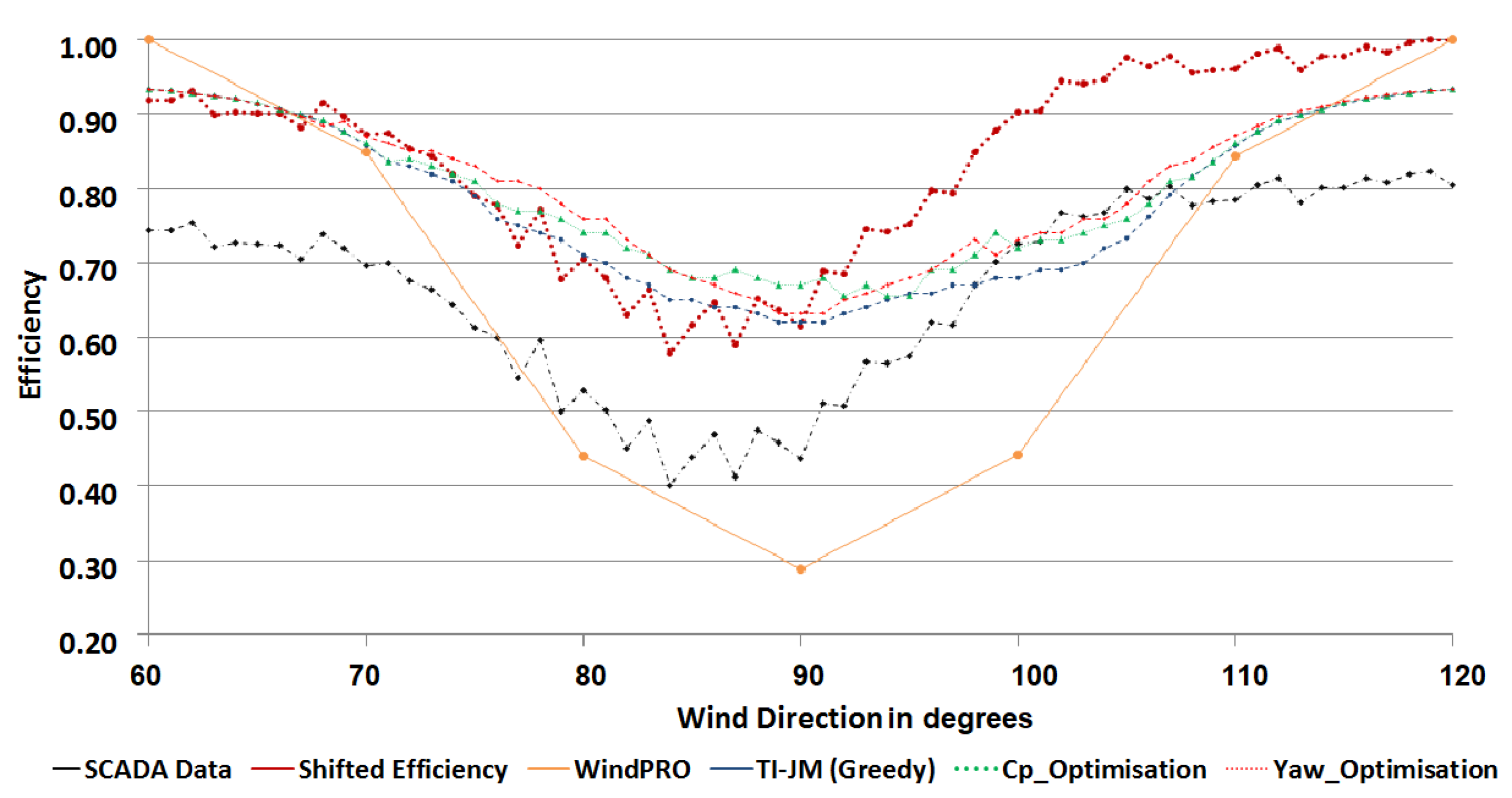
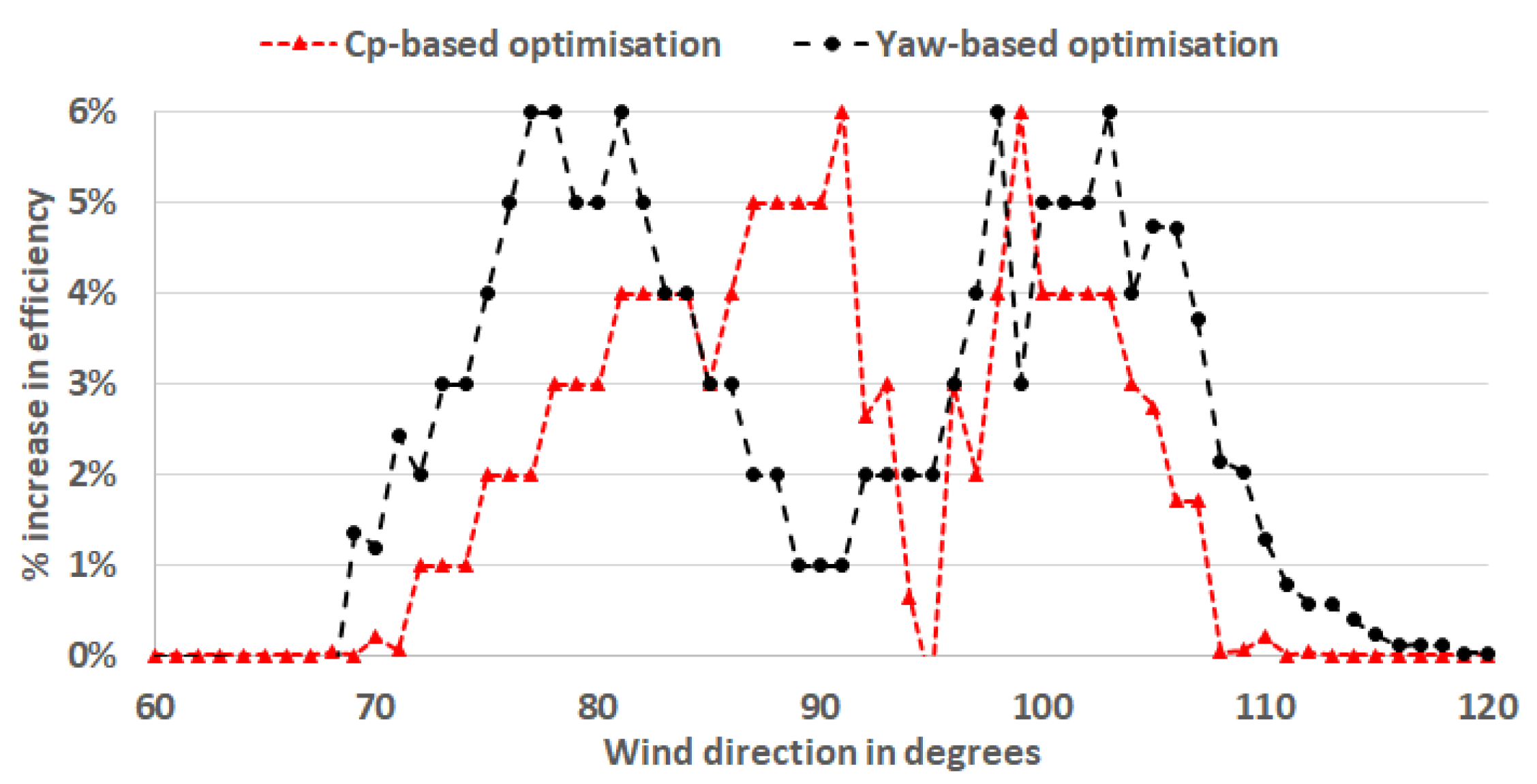
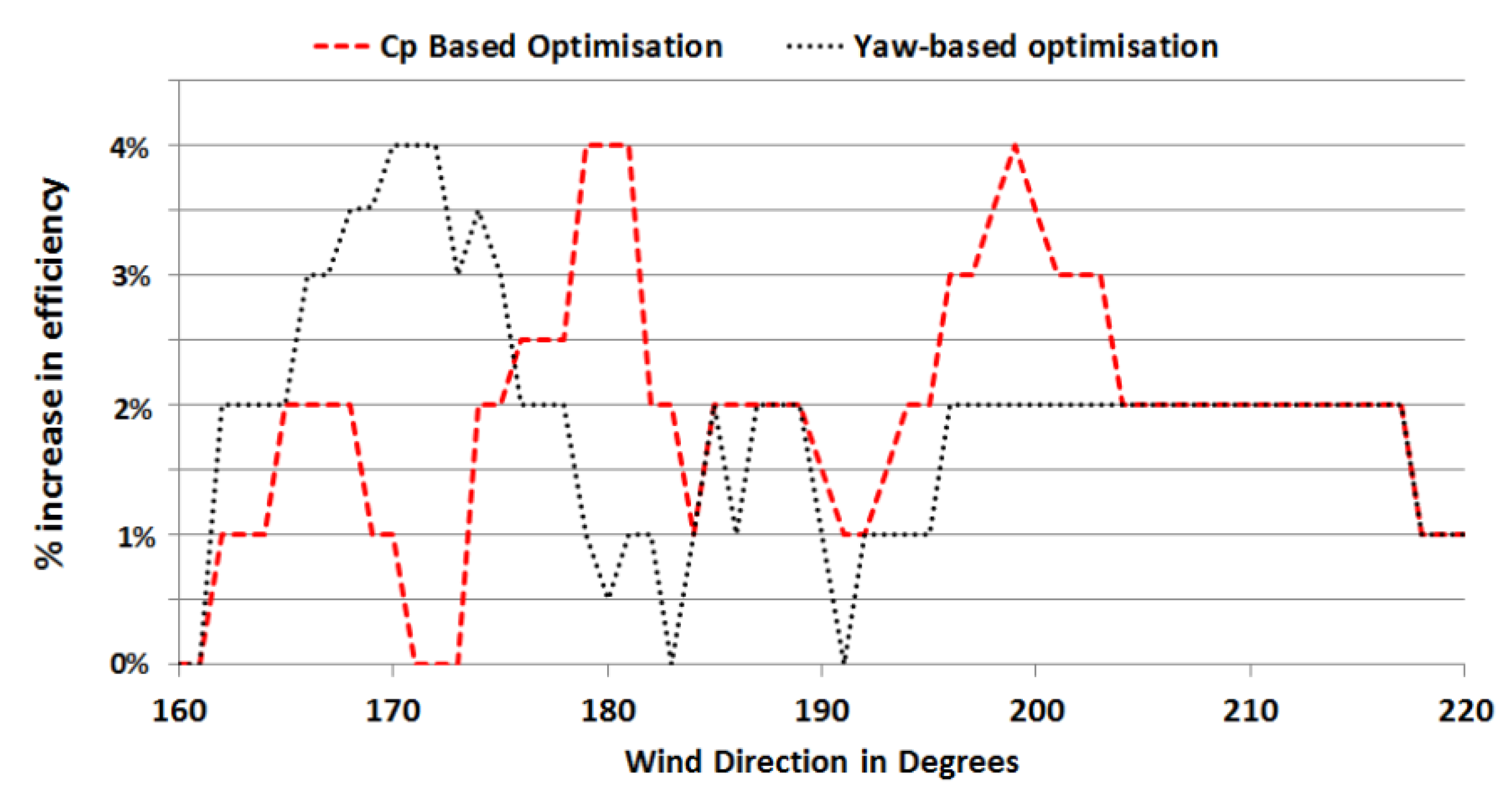
Wake effects are negligible in above-rated conditions [5], hence only below-rated conditions were assumed in the simulations in this section. Efficiencies based on WindPRO and real-time SCADA data in full or near-full wake conditions were used as benchmarks. WindPRO direction bin was kept at 10°, which is the finest possible. WindPRO uses the standard onshore and offshore values of k given in [71], for wake estimation. TI–JM used SCADA data for Brazos-row and SMV for tuning the initial value of k according to the conditions. For TI–JM and SCADA data, the directional resolution was maintained at 1°. TI–JM was first compared with SCADA data and WindPRO using efficiencies based on greedy control. The optimal control strategies were then evaluated by comparing them with greedy control using TI–JM. Contour plots of the three wind farm case studies in full wake conditions were used for depicting a comparison of conventional and coordinated control strategies.
Data filtering was applied to ensure that only operational turbines were analysed. It was observed that the maximum efficiency in no-wake conditions for Brazos-row and SMV wind farms was not 100%. Instead it was 82% for Brazos-row and 86% for SMV. These discrepancies may have been caused by anomalies in SCADA data or other unknown operational issues. WindPRO and TI–JM did not consider any anomalies or issues with data, taking only wake effects for wind deficit estimation. Therefore, the maximum efficiency (82% for Brazos-row and 86% for SMV) was shifted to 100% by simply adding the difference (18% for Brazos-row, 14% for SMV) to the efficiency at all points. This nullified the impact of all other issues by taking into consideration only the impact of wake effects on farms productions. The shifted efficiency (based on SCADA data) was then compared, with efficiencies obtained with WindPRO and TI–JM.
Results and analyses for Brazos-row, SMV and Lillgrund wind farms were presented in Section 7.1, Section 7.2, and Section 7.3 respectively. These results were obtained using a basic computer (4 cores, 3.50 GHz processor and 16 GB RAM).

7.1. Brazos-Row

Efficiency of the Brazos-row was calculated using SCADA data from 2004–2006 provided by [72]. The case study row was under wake effects in the directional sector of 90 ° ± 30 ° . Figure 5 depicts the average efficiency in this directional sector. The sector 90 ° ± 30 ° can be further divided into bins as follows.
  • Full wakes (worst case) = 90 ° ± 10 °
  • Partial wakes = 110 ° ± 10 ° and 70 ° ± 10 °
The shifted efficiency in Figure 5 shows that efficiency can drop to as low as 58% in full wake conditions. WindPRO and TI–JM estimated that efficiency can be as low as 30% and 62% in full wake conditions. The standard Jensen model available in WindPRO was used with a constant k = 0.07 , for such an onshore terrain. WindPRO uses the WAsP model [31] for analysing the impact of terrain on wake effects. On the other hand, TI–JM did not use any terrain model, rather it varied k according to wind conditions, instead of keeping it constant as discussed in Section 3. TI–JM used k up to 0.25 for estimating wind speed deficits inside the farm. The initial value of k was the standard k for such terrains. Wind direction was derived from the data obtained from met mast.
It can be seen in Figure 5 that WindPRO and TI–JM predict almost symmetrical efficiencies around 90° as it is a straight line (row) of turbines (Figure 2a). However, the shifted efficiencies were not symmetrical on both sides of 90°. The efficiency predicted by TI–JM fit well with the shifted efficiency in the 60°–90° sector. However, the efficiency was not that accurate in the 91°–120° sector. Overall, TI–JM predicted better than WindPRO in most of the cases. TI–JM and WindPRO ignored wake-meandering and wind shear effects, which can result in uncertainty in models’ prediction accuracy.
Both C P and yaw-based optimised strategies can increase the average efficiency by up to 6% as compared to greedy control as can be seen in Figure 5 and Figure 6. It was observed that coordinated control based on C p optimisation performed better in full or near-full wake conditions. Yaw optimisation can produce better results in partial wake conditions.
The reduction in C P of upstream turbines depended upon wind speed and direction. Optimised reduction in C P of the upstream turbines for curtailing their power production ranged between 3% and 20%. In higher wind speeds, the C P curtailment was minimal as wake effects were also minimal. This was true for all the three wind farm case studies. In full wake conditions, significantly larger yaw-offset (up to ± 30 ° ) was required for deflecting the wake away from the swept area of the wake affected turbines. This converted a full wake into a partial wake for the downstream turbines but at the same time it significantly reduced the production of the yawed turbine. A partial wake was converted into a minimal or no-wake situation using a yaw-offset in a range of ± 15 ° , producing a significant increase in wake affected turbines’ productions. The impact of this yaw-offset on the yawed turbine was considerably low, hence increase in net production was observed.
Wind flow with state of the art greedy control, C P and yaw-based optimised strategies in full wake conditions is shown in Figure 7. The lower wind speed deficit inside the wind farm with C P optimisation, as compared to greedy control can also be seen. Figure 7c depicts the wake skewing from the downstream turbines. The wake-added turbulence intensity increased k, hence the wake spread inside the farm as shown in Figure 7. The optimisation process (in a single simulation) took less than 15 s for Brazos-row.

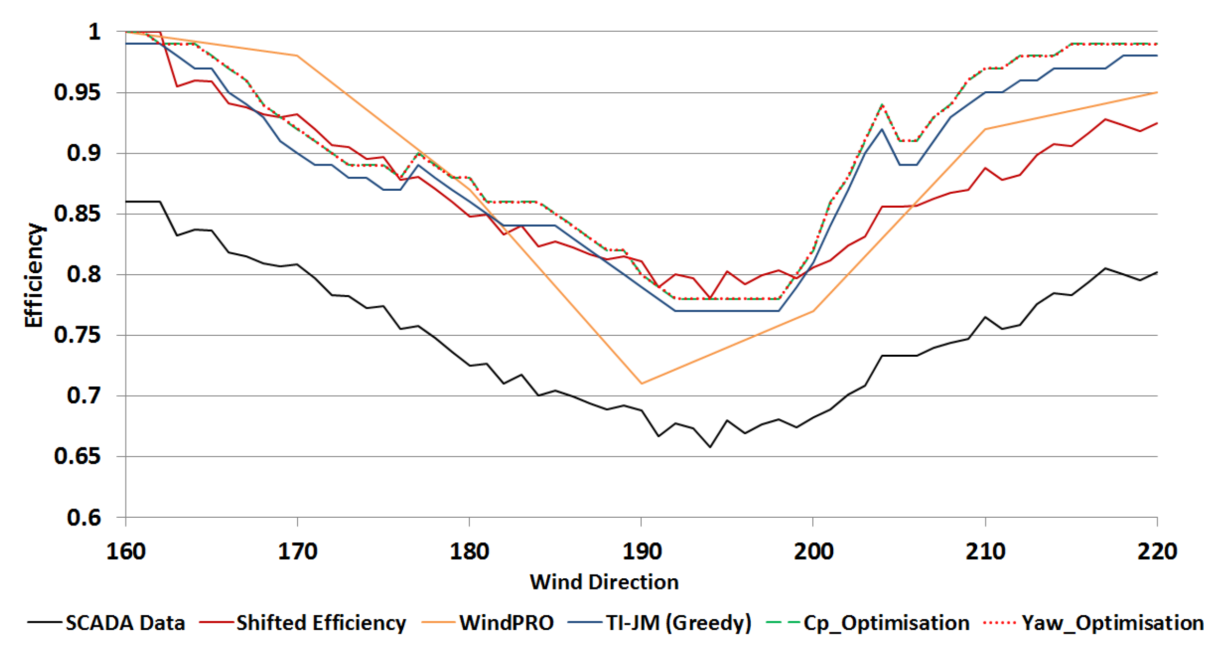
7.2. Le Sole de Moulin Vieux (SMV)
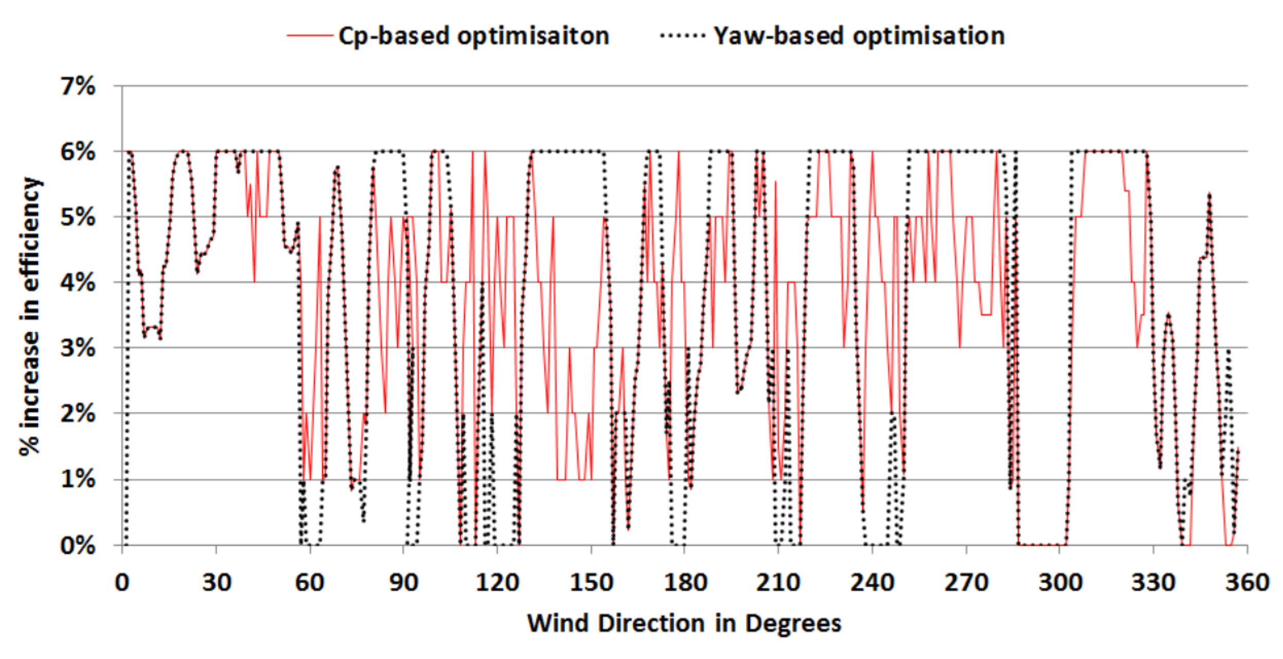
SCADA data of the SMV wind farm from 2011–2014 was provided by Maïa Eolis (now Engie Green). Full or near-full wake conditions were assumed in the simulations. Average efficiency from the south 160°–220° is shown in Figure 8. The sector 160°–220° was chosen because of the prevailing wind direction and significant wake effects observed in these directions. Analyses of the SCADA data showed that shifted efficiency can drop to 78% in the worst conditions. WindPRO (standard Jensen model with k = 0.07 and WAsP) predicted that efficiency can be as low as 70% with such layout and terrain. TI–JM estimated a minimum efficiency of 76% in the worst case. It was observed that k can increase up to 0.20 as the wind moves through the wind farm.
It can be observed in Figure 8 that TI–JM matches the shifted efficiency better in 160°–200°, while WindPRO produces better results in 200°–220°. TI–JM under-estimated wake losses in the 200°–220° sector, concluding that the k needs to be further increased in this sector for better wake estimation. Wind conditions on site due to the nearby woods (Section 5.2) also added to the complexity for wind deficit prediction.
It can be observed in Figure 8 and Figure 9 that optimised control strategies can increase efficiency by up to 4%. The directional sector 160°–220° could not be divided into partial and full wakes for the whole wind farm in this case. Turbines in the SMV were not installed in a straight line (Figure 3a), hence these turbines will be under different wake conditions for a given wind direction [8]. SMV5 produced full wakes on SMV1-SMV4 in 180 ° ± 10 ° . For the same wind direction, SMV5 was under minimal wake effects of SMV6 and SMV6 was under negligible wake effects of SMV7. SMV6 experienced significant wake effects of SMV7 in 200 ° ± 10 ° but at the same time all other turbines experienced minimal wake effects from their corresponding upstream turbines. The optimised yaw-offsets and C P curtailment settings were the same as for Brazos-row (Section 7.1).
A comparison of wind flow using conventional and optimised control strategies is shown in Figure 10. The optimisation process (in a single simulation) took less than 15 s for SMV.

7.3. Lillgrund

Lillgrund efficiency can be as low as 40% in the worst case, when turbines were under full wake effects [5]. Due to the dense layout of the farm, turbines experienced wake effects in almost all wind directions. Therefore, the 360° farm efficiency curve available in [5] was digitised using [73] and reproduced in Figure 11. Other details such as farm layout, surface roughness length, turbine characteristics, and turbulence intensity were provided by [70]. As per [70], the value of k was tuned for best fit as required by the wake model. It was noted in the simulations that values of k in Equation (11) provided the best fit (for TI–JM) with actual efficiency. WindPRO used the standard k = 0.04 for offshore wind conditions in this case. Although WindPRO captured the shape of the efficiency curve, in most of the cases it underestimated wake effects. On the other hand, TI–JM predicted wake effects with almost 95% accuracy in this case.
k = 0.04 i f u 0 7.0 m / s k = 0.08 i f 7.0 m / s < u 0 12.0 m / s
wind speeds > 12 not considered as suggested in [5].
Dense wind farms such as Lillgrund can significantly benefit from coordinated control. Full wake conditions were experienced when the wind flowed in 45 ° ± 10 ° , 135 ° ± 10 ° , 225 ° ± 10 ° , 315 ° ± 10 ° directions. It can be seen in Figure 12 that efficiency can be improved by a maximum of 6% with optimised control strategies. It can also be observed in Figure 12 that efficiency can be increased in almost all wind directions as wake effects were always present in the farm. In partial wakes, yaw-based optimisation provided a better opportunity for efficiency improvement while C P optimisation was more suitable in full wake conditions. This observation was same as for Brazos-row. The ranges for C P curtailment and yaw-offsets were the same as Brazos-row and SMV.
A comparison of wind flow using conventional and optimised control strategies is shown in Figure 13. The optimisation process (in a single simulation) took less than 50 s for Lillgrund.

8. Conclusions

Wake effects can have a significant impact on economic performance of wind farms by increasing production losses and fatigue loads. This work presented an intelligent and fast-processing farm controller for reducing wake effects. Optimised coordinated control strategies are used for increasing farm production by optimally varying C P or yaw-angles. The optimised control strategies used TI–JM for estimating wind speeds inside the wind farms and PSO for optimisation. TI–JM is an improved version of the standard Jensen model. TI–JM takes deep array effects into consideration using wake added turbulence intensity for estimating k. It can accurately predict wind speed inside a wind farm in most of the cases in the wind farm case studies, and hence farm production and efficiency. Both the C P -based and yaw-based optimised strategies increased wind farm efficiency as compared to the conventional greedy control. The system has been designed for all wind conditions, however it was tested only for static wind conditions using TI–JM. Simulations confirm that average efficiency can be increased by up to 6% for Brazos-row and Lillgrund while 4% for SMV. SMV and Brazos-row were optimised in a maximum of 15 s while Lillgrund always took less than 50 s, using a basic computer. It is concluded that C P optimisation is suitable in full wake conditions for net production maximisation. Yaw-optimisation is beneficial for farm production maximisation in partial wake conditions. As future work, these results shall be validated using high fidelity wake models. It shall be noted that yaw optimisation increases fatigue loading on the yawed turbines. The aim of this paper is only to analyse production maximisation. Fatigue load optimisation would require a multi-objective optimisation for minimising loads and maximising production of the farm, which is left for future work. Furthermore, a wind turbine has a designed service life of almost 20 to 25 years, however due to the technological advances and ever-growing size of turbines, farm operators replace these turbines much earlier than their end of life. Hence, the increase in fatigue loading for some gain in production might be economically beneficial. This can be further investigated in the future.

Author Contributions

This work is primarily based on the PhD research work of T.A. at Durham University, UK. This PhD work was supervised by P.C.M. and B.K. A.B. provided support in the data analyses section. J.A. helped in visualisation of the results through her Masters Thesis. O.C. provided assistance in using WindPRO and obtaining data for the Lillgrund wind farm.

Funding

This research was funded by the Commonwealth Scholarship Commission (CSC), UK (reference: PKCS-2013-384) and The US Pakistan Center for Advanced Studies in Energy, University of Engineering and Technology Peshawar, Pakistan.

Conflicts of Interest

The authors declare no conflict of interest.

Abbreviations

The following abbreviations are used in this manuscript:
PSOParticle Swarm Optimisation
TI–JMTurbulence Intensity based Jensen Model
SMVLe Sole de Moulin Vieux
CFDComputational Fluid Dynamics
SCADASupervisory Control And Data Acquisition

References

  1. Bitar, E.; Seiler, P. Coordinated control of a wind turbine array for power maximization. In Proceedings of the 2013 American Control Conference (ACC), Washington, DC, USA, 17–19 June 2013; pp. 2898–2904. [Google Scholar]
  2. Pao, L.Y.; Johnson, K.E. A tutorial on the dynamics and control of wind turbines and wind farms. In Proceedings of the American Control Conference (ACC ’09), St. Louis, MO, USA, 10–12 June 2009; Volume 172, pp. 2076–2089. [Google Scholar]
  3. Johnson, K.E.; Thomas, N. Wind farm control: addressing the aerodynamic interaction among wind turbines. In Proceedings of the American Control Conference (ACC ’09), St. Louis, MO, USA, 10–12 June 2009; Volume 155, pp. 2104–2109. [Google Scholar]
  4. Ahmad, T.; Girard, N.; Kazemtabrizi, B.; Matthews, P. Analysis of Two Onshore Wind Farms with a Dynamic Farm Controller; EWEA: Paris, France, 2015. [Google Scholar]
  5. Dahlberg, J.A. Assessment of the Lillgrund Windfarm: Power Performance; Technical Report 21858-1; Vatenfall Vindkraft AB: Solna Municipality, Sweden, 2009; Available online: https://corporate.vattenfall.se/globalassets/sverige/om-vattenfall/om-oss/var-verksamhet/vindkraft/lillgrund/assessment.pdf (accessed on 6 February 2019).
  6. Aranda, F.A. Wind Farm Control Methods, IEA R&D Wind Task 11—Topical Expert Meeting; Technical Report; International Energy Agency: Solna, Sweden, 2012. [Google Scholar]
  7. Ahmad, T. Wind Farm Coordinated Control and Optimisation. Ph.D. Thesis, School of Engineering & Computing Sciences, Durham University, Durham, UK, 2017. Available online: http://etheses.dur.ac.uk/12323/1/Tanvir_Thesis_Final_Submission.pdf (accessed on 6 February 2019).
  8. Ahmad, T.; Coupiac, O.; Pettit, A.; Guignard, S.; Girard, N.; Kazemtabrizi, B.; Matthews, P. Field Implementation and Trial of Coordinated Control of Wind Farms. IEEE Trans. Sustain. Energy 2018, 9, 1169–1176. [Google Scholar] [CrossRef]
  9. Ambekar, A.; Ryali, V.; Tiwari, A.K. Methods and Systems for Optimizing Farm-Level Metrics in a Wind Farm. U.S. Patent 9,201,410, 1 December 2015. [Google Scholar]
  10. Soleimanzadeh, M.; Wisniewski, R.; Kanev, S. An optimization framework for load and power distribution in wind farms. J. Wind Eng. Ind. Aerodyn. 2012, 107, 256–262. [Google Scholar] [CrossRef]
  11. Lignarolo, L.; Ragni, D.; Krishnaswami, C.; Chen, Q.; Simão Ferreira, C.; van Bussel, G. Experimental analysis of the wake of a horizontal-axis wind-turbine model. Renew. Energy 2014, 70, 31–46. [Google Scholar] [CrossRef]
  12. Sanderse, B. Aerodynamics of Wind Turbine Wakes; Tech. Rep ECN-E–09-016; Energy Research Center of the Netherlands (ECN): Petten, The Netherlands, 2009. [Google Scholar]
  13. Barthelmie, R.; Larsen, G.; Frandsen, S.; Folkerts, L.; Rados, K.; Pryor, S.; Lange, B.; Schepers, G. Comparison of Wake Model Simulations with Offshore Wind Turbine Wake Profiles Measured by Sodar. J. Atmos. Ocean. Technol. 2006, 23, 888–901. [Google Scholar] [CrossRef]
  14. Gaumond, M.; Réthoré, P.E.; Bechmann, A.; Ott, S.; Larsen, G.C.; Peña, A.; Hansen, K.S. Benchmarking of wind turbine wake models in large offshore wind farms. In Proceedings of the Science of Making Torque from Wind Conference, Oldenburg, Germany, 8–10 October 2012. [Google Scholar]
  15. Vogstad, K.; Bhutoria, V.; Lund, J.A.; Ivanell, S.; Uzunoglu, B. Instant Wind—Model Reduction for Fast CFD Computations; Elforsk Report 12:72. 2012. Available online: https://www.researchgate.net/publication/236222690_Instant_Wind_Model_reduction_for_fast_CFD_computations_Elforsk_report_1272 (accessed on 6 February 2019).
  16. Annoni, J.; Seiler, P.; Johnson, K.; Fleming, P.; Gebraad, P. Evaluating wake models for wind farm control. In Proceedings of the American Control Conference (ACC), Portland, OR, USA, 4–6 June 2014; pp. 2517–2523. [Google Scholar]
  17. Rados, K.; Larsen, G.; Barthelmie, R.; Schlez, W.; Lange, B.; Schepers, G.; Hegberg, T.; Magnisson, M. Comparison of wake models with data for offshore windfarms. Wind Eng. 2001, 25, 271–280. [Google Scholar] [CrossRef]
  18. Vermeer, L.; Sørensen, J.N.; Crespo, A. Wind turbine wake aerodynamics. Prog. Aerosp. Sci. 2003, 39, 467–510. [Google Scholar] [CrossRef]
  19. Franke, J.; Hirsch, C.; Jensen, A.; Krüs, H.; Schatzmann, M.; Westbury, P.; Miles, S.; Wisse, J.; Wright, N. Recommendations on the use of CFD in wind engineering. Cost Action C 2004, 14, C1. [Google Scholar]
  20. Ainslie, J.F. Calculating the flowfield in the wake of wind turbines. J. Wind Eng. Ind. Aerodyn. 1988, 27, 213–224. [Google Scholar] [CrossRef]
  21. Churchfield, M.J.; Moriarty, P.J.; Hao, Y.; Lackner, M.A.; Barthelmie, R.; Lundquist, J.K.; Oxley, G.S. A comparison of the dynamic wake meandering model, large-eddy simulation, and field data at the Egmond aan Zee Offshore wind plant. In Proceedings of the AIAA Science and Technology Forum and Exposition (SciTech 2015), Kissimmee, FL, USA, 5–9 January 2015. [Google Scholar]
  22. Sanderse, B.; Pijl, S.; Koren, B. Review of Computational Fluid Dynamics for wind turbine wake aerodynamics. Wind Energy 2011, 14, 799–819. [Google Scholar] [CrossRef]
  23. Hoelzer, M.; Hölling, M.; Wolken-Möhlmann, G.; Knebel, P.; Gottschall, J.; Anahua, E.; Barth, S.; Peinke, J. Annual Report 2007—Research Projects (RP); Technical Report; ForWind—Center for Wind Energy Research of the Universities of Oldenburg and Hannover: Oldenburg, Germany, 2007. [Google Scholar]
  24. Churchfield, M. Review of Wind Turbine Wake Models and Future Directions (Presentation); Technical Report NREL/PR-5000-60208; National Renewable Energy Laboratory (NREL): Golden, CO, USA, 2013.
  25. Jensen, N.O. A Note on Wind Generator Interaction; Technical Report Risø -M-2411; Risø National Laboratory: Roskilde, Denmark, 1983. [Google Scholar]
  26. Katic, I.; Højstrup, J.; Jensen, N.O. A simple model for cluster efficiency. In Proceedings of the European Wind Energy Association Conference and Exhibition, Rome, Italy, 7–9 October 1986; pp. 407–410. [Google Scholar]
  27. Larsen, G.C.; Aagaard Madsen, H.; Sørensen, N.N. Mean wake deficit in the near field. In Proceedings of the European Wind Energy Conference and Exhibition, Madrid, Spain, 16–19 June 2003; European Wind Energy Association (EWEA): Brussels, Belgium, 2003. [Google Scholar]
  28. Frandsen, S.; Barthelmie, R.; Pryor, S.; Rathmann, O.; Larsen, S.; Højstrup, J.; Thøgersen, M. Analytical modelling of wind speed deficit in large offshore wind farms. Wind Energy 2006, 9, 39–53. [Google Scholar] [CrossRef]
  29. Annoni, J.; Gebraad, P.M.; Scholbrock, A.K.; Fleming, P.A.; van Wingerden, J.W. Analysis of axial-induction- based wind plant control using an engineering and a high-order wind plant model. Wind Energy 2015, 19, 1135–1150. [Google Scholar] [CrossRef]
  30. Barthelmie, R.J.; Rathmann, O.; Frandsen, S.T.; Hansen, K.; Politis, E.; Prospathopoulos, J.; Rados, K.; Cabezón, D.; Schlez, W.; Phillips, J.; et al. Modelling and measurements of wakes in large wind farms. J. Phys. Conf. Ser. 2007, 75, 012049. [Google Scholar] [CrossRef] [Green Version]
  31. Nielsen, P.; Villadsen, J.; Kobberup, J.; Madsen, P.; Jacobsen, T.; Thøgersen, M.L.; Sørensen, M.V.; Sørensen, T.; Svenningsen, L.; Motta, M.; et al. WindPRO 2.7 User Guide, 3rd ed.; EMD International A/S: Aalborg, Denmark, 2010. [Google Scholar]
  32. Beaucage, P.; Robinson, N.; Brower, M.; Alonge, C. Overview of six commercial and research wake models for large offshore wind farms. In Proceedings of the European Wind Energy Association Conference, Copenhagen, Denmark, 16–19 March 2012; pp. 95–99. [Google Scholar]
  33. Hassan, G. WindFarmer 5.3: Theory Manual; Garrad Hassan & Partners Ltd. DNV GL-Energy: Bristol, England, 2014. [Google Scholar]
  34. Zigras, D.; Moennich, K. Farm efficiencies in large wind farms. In Proceedings of the German Wind Energy Conference, Berlin, Germany, 28–30 July 2006. [Google Scholar]
  35. Manwell, J.F.; McGowan, J.G.; Rogers, A.L. Wind Energy Explained: Theory, Design and Application; John Wiley & Sons: West Sussex, UK, 2010. [Google Scholar]
  36. Sidewell, N.; Ahmad, T.; Matthews, P.C. Onshore Wind Farm Fast Wake Estimation Method: Critical Analysis of the Jensen Model; EWEA: Paris, France, 2015. [Google Scholar]
  37. Vogstad, K.; Bhutoria, V.; Lund, J.A.; Ivanell, S. Instant Wind Model Reduction for Fast CFD Computations; Technical Report 12:72; Elforsk: Stockholm, Sweden, 2012; Available online: https://uu.diva-portal.org/smash/get/diva2:924368/FULLTEXT01.pdf (accessed on 6 February 2019).
  38. Renkema, D.J. Validation of Wind Turbine Wake Models. Master’s Thesis, Faculty of Aerospace Engineering, TU Delft, Delft, The Netherlands, 2007. [Google Scholar]
  39. Park, J.; Kwon, S.; Law, K.H. Wind Farm Power Maximization Based on a Cooperative Static Game Approach. Available online: https://pdfs.semanticscholar.org/8fa6/c5709a61edd3a54e9a09303086fa93d73e2d.pdf (accessed on 6 February 2019).
  40. Ahmad, T.; Matthews, P.; Kazemtabrizi, B. PSO Based Wind Farm Controller. In Proceedings of the 11th Edition of the International Conference on Evolutionary and Deterministic Methods for Design, Optimization and Control with Applications to Industrial and Societal Problems (EUROGEN-2015), Glasgow, UK, 14–16 September 2015; pp. 277–283. [Google Scholar]
  41. González, J.S.; Payán, M.B.; Santos, J.R.; Rodríguez, Á.G.G. Maximizing the overall production of wind farms by setting the individual operating point of wind turbines. Renew. Energy 2015, 80, 219–229. [Google Scholar] [CrossRef]
  42. Marden, J.R.; Ruben, S.D.; Pao, L.Y. Surveying game theoretic approaches for wind farm optimization. In Proceedings of the AIAA Aerospace Sciences Meeting, Nashville, TN, USA, 9–12 January 2012; pp. 1–10. [Google Scholar]
  43. Burton, T.; Sharpe, D.; Jenkins, N.; Bossanyi, E. Wind Energy Handbook; John Wiley & Sons: Hoboken, NJ, USA, 2001. [Google Scholar]
  44. Steinbuch, M.; de Boer, W.; Bosgra, O.; Peters, S.; Ploeg, J. Optimal control of wind power plants. J. Wind Eng. Ind. Aerodyn. 1988, 27, 237–246. [Google Scholar] [CrossRef]
  45. Corten, G.; Schaak, P.; Bot, E. More power and less loads in wind farms: Heat and Flux. In Proceedings of the European Wind Energy Conference & Exhibition, London, UK, 22–25 November 2004. [Google Scholar]
  46. Soleimanzadeh, M.; Brand, A.J.; Wisniewski, R. A wind farm controller for load and power optimization in a farm. In Proceedings of the 2011 IEEE International Symposium on Computer-Aided Control System Design (CACSD), Denver, CO, USA, 28–30 September 2011; Volume 186, pp. 1202–1207. [Google Scholar]
  47. Soleimanzadeh, M.; Wisniewski, R. Controller design for a wind farm, considering both power and load aspects. Mechatronics 2011, 21, 720–727. [Google Scholar] [CrossRef]
  48. Odgaard, P.F.; Baekgaard, M.; Astrup, B. Model based control of wind parks. In Proceedings of the EWEC Conference, Warsaw, Poland, 20–23 April 2010. [Google Scholar]
  49. Spudic, V.; Jelavic, M.; Baotic, M.; Peric, N. Hierarchical wind farm control for power/load optimization. In Proceedings of the Science of making Torque from Wind (Torque2010), Heraklion, Greece, 28–30 June 2010. [Google Scholar]
  50. Spudic, V.; Baotic, M.; Peric, N. Wind farm load reduction via parametric programming based controller design. In Proceedings of the 18th IFAC World Congress, Milan, Italy, 28 August–2 September 2011. [Google Scholar]
  51. Spudić, V.; Jelavić, M.; Baotić, M. Wind turbine power references in coordinated control of wind farms. Automatika 2011, 52, 82–94. [Google Scholar] [CrossRef]
  52. Gebraad, P.; Teeuwisse, F.; Van Wingerden, J.; Fleming, P.A.; Ruben, S.; Marden, J.; Pao, L. Wind plant power optimization through yaw control using a parametric model for wake effects—A CFD simulation study. Wind Energy 2016, 19, 95–114. [Google Scholar] [CrossRef]
  53. Gebraad, P.; van Wingerden, J. Maximum power-point tracking control for wind farms. Wind Energy 2015, 18, 429–447. [Google Scholar] [CrossRef]
  54. Spruce, C.J. Simulation and Control of Windfarms. Ph.D. Thesis, University of Oxford, Oxford, UK, 1993. [Google Scholar]
  55. Knudsen, T.; Bak, T.; Svenstrup, M. Survey of wind farm control power and fatigue optimization. Wind Energy 2015, 18, 1333–1351. [Google Scholar] [CrossRef]
  56. Qian, G.W.; Ishihara, T. A New Analytical Wake Model for Yawed Wind Turbines. Energies 2018, 11, 665. [Google Scholar] [CrossRef]
  57. Marathe, N.; Swift, A.; Hirth, B.; Walker, R.; Schroeder, J. Characterizing power performance and wake of a wind turbine under yaw and blade pitch. Wind Energy 2016, 19, 963–978. [Google Scholar] [CrossRef]
  58. Wan, S.; Cheng, L.; Sheng, X. Effects of yaw error on wind turbine running characteristics based on the equivalent wind speed model. Energies 2015, 8, 6286–6301. [Google Scholar] [CrossRef]
  59. Park, J.; Law, K.H. A data-driven, cooperative wind farm control to maximize the total power production. Appl. Energy 2016, 165, 151–165. [Google Scholar] [CrossRef]
  60. Boorsma, K. Power and Loads for Wind Turbines in Yawed Conditions; Technical Report, ECN-E-12-047; ECN: Petten, The Netherlands, 2012. [Google Scholar]
  61. Annoni, J.; Fleming, P.; Scholbrock, A.; Roadman, J.; Dana, S.; Adcock, C.; Porte-Agel, F.; Raach, S.; Haizmann, F.; Schlipf, D. Analysis of Control-Oriented Wake Modeling Tools Using Lidar Field Results; National Renewable Energy Lab. (NREL): Golden, CO, USA, 2018.
  62. Wagenaar, J.; Machielse, L.; Schepers, J. Controlling wind in ECN scaled wind farm. In Proceedings of the Europe Premier Wind Energy Event, Copenhagen, Denmark, 16–19 April 2012; pp. 685–694. [Google Scholar]
  63. Schram, C.; Vyas, P. Windpark Turbine Control System and Method for Wind Condition Estimation and Performance Optimization. U.S. Patent App. 11/288,081, 31 May 2007. [Google Scholar]
  64. Kanev, S.; Savenije, F. Active Wake Control: Loads Trends; Technical Report ECN-E–15-004; ECN: Petten, The Netherlands, 2015. [Google Scholar]
  65. Kennedy, J.; Eberhart, R. Particle swarm optimization. In Proceedings of the IEEE International Conference on Neural Networks, Perth, Australia, 27 November–1 December 1995; Volume 4, pp. 1942–1948. [Google Scholar]
  66. Kennedy, J. Small worlds and mega-minds: Effects of neighborhood topology on particle swarm performance. In Proceedings of the 1999 Congress on Evolutionary Computation (CEC 99), Washington, DC, USA, 6–9 July 1999; Volume 3. [Google Scholar]
  67. Kennedy, J.; Mendes, R. Population structure and particle swarm performance. In Proceedings of the 2002 Congress on Evolutionary Computation, Honolulu, HI, USA, 12–17 May 2002; Available online: http://repositorium.sdum.uminho.pt/bitstream/1822/2291/1/wcci2002.pdf (accessed on 6 February 2019).
  68. Shi, Y. Particle swarm optimization. IEEE Connect. 2004, 2, 8–13. [Google Scholar]
  69. Rienecker, M.M.; Suarez, M.J.; Gelaro, R.; Todling, R.; Bacmeister, J.; Liu, E.; Bosilovich, M.G.; Schubert, S.D.; Takacs, L.; Kim, G.K.; et al. MERRA: NASA’s modern-era retrospective analysis for research and applications. J. Clim. 2011, 24, 3624–3648. [Google Scholar] [CrossRef]
  70. Moriarty, P.; Rodrigo, J.S.; Gancarski, P.; Chuchfield, M.; Naughton, J.W.; Hansen, K.S.; Machefaux, E.; Maguire, E.; Castellani, F.; Terzi, L.; et al. IEA-Task 31 WAKEBENCH: Towards a protocol for wind farm flow model evaluation. Part 2: Wind farm wake models. J. Phys. Conf. Ser. 2014, 524, 012185. [Google Scholar] [CrossRef] [Green Version]
  71. Thørgersen, M.; Sørensen, T.; Nielsen, P.; Grötzner, A.; Chun, S. WindPRO/PARK: Introduction to Wind Turbine Wake Modelling and Wake Generated Turbulence; EMD International A/S: Aalborg, Denmark, 2005; Available online: http://www.emd.dk/files/windpro/manuals/for_print/Appendices-all_UK.pdf (accessed on 6 February 2019).
  72. Bueno Gayo, J. ReliaWind Project Final Report; Technical Report Project Nr 212966; Gamesa Innovation and Technology: 2011. Available online: https://setis.ec.europa.eu/energy-research/sites/default/files/project/docs/Publishable%20Summary%20-%20110513_Reliawind_Final%20Publishable%20Summary%20to%20EC.pdf (accessed on 6 February 2019).
  73. Rohatgi, A. WebPlotDigitizer. Available online: http://arohatgi.info/WebPlotDigitizer/ (accessed on 1 February 2019).
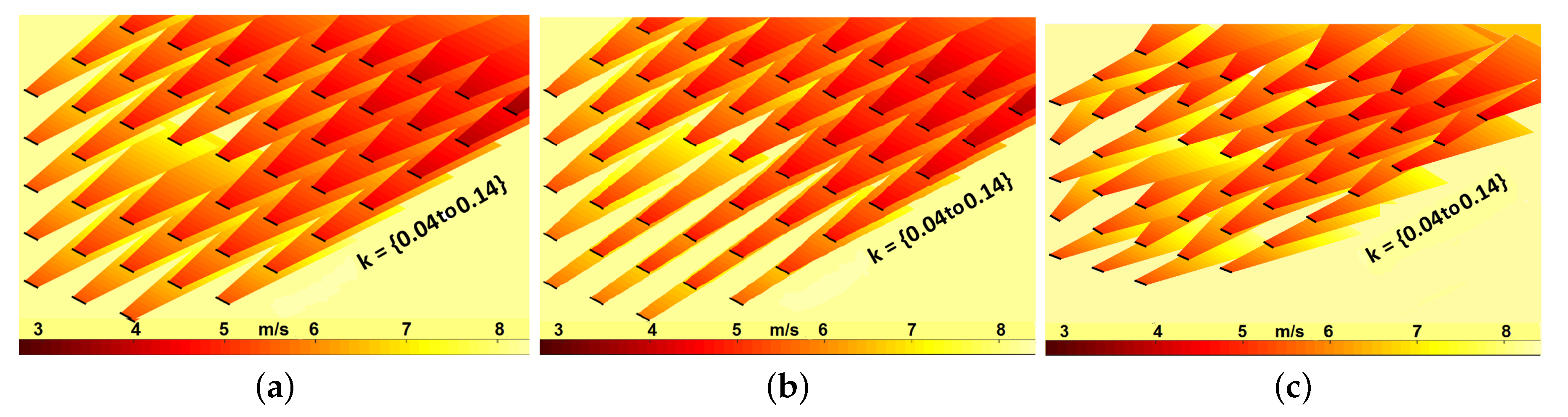
Figure 1. Particle swarm optimisation (PSO) flowchart for solving the coordinated control problem.
Energies 12 00544 g001
Figure 2. (a) Brazos layout (case study row encircled); (b) Wind–rose obtained with data from 2004–2006.
Energies 12 00544 g002
Figure 3. (a) Layout of the Le Sole de Moulin Vieux (SMV) wind farm; (b) Wind–rose obtained with data from 2011–2015.
Energies 12 00544 g003
Figure 4. (a) Lillgrund layout and turbines in set j; (b) Wind–rose obtained with data from 2000–2015.
Energies 12 00544 g004
Figure 5. Brazos efficiency in 60°–120° directional sector.
Energies 12 00544 g005
Figure 6. Impact (% increase) of optimised control strategies on Brazos-row efficiency, relative to greedy control.
Energies 12 00544 g006
Figure 7. Comparison of control strategies for Brazos-row at 8 m/s in full wakes. Range of k varies from 0.07 (free-stream) to 0.025 (deep inside the farm); (a) Conventional greedy control; (b) Optimised control based on C P ; (c) Optimised control based on yaw-offset.
Energies 12 00544 g007
Figure 8. SMV Efficiency in 160°–220° sector.
Energies 12 00544 g008
Figure 9. Impact (% increase) of optimised control strategies on SMV efficiency, relative to greedy control.
Energies 12 00544 g009
Figure 10. Comparison of control strategies for SMV at 8 m/s from north. Range of k varies from 0.07 (free-stream) to 0.020 (deep inside the farm); (a) Conventional greedy control; (b) Optimised control based on C P ; (c) Optimised control based on yaw-offset.
Energies 12 00544 g010
Figure 11. Average 360° efficiency of Lillgrund in below-rated conditions.
Energies 12 00544 g011
Figure 12. Impact (% increase) of optimised control strategies on Lillgrund efficiency, relative to greedy control.
Energies 12 00544 g012
Figure 13. Comparison of control strategies for Lillgrund at 8 m/s in full wake conditions. Range of k varies from 0.04 (free-stream) to 0.14 (deep inside the farm); (a) Conventional greedy control; (b) Optimised control based on C P ; (c) Optimised control based on yaw-offset.
Energies 12 00544 g013
Table 1. Turbines in set j.
Wind DirectionFigure 4a N j j
North-west N N W 3Row-8 (3 turbines)
South-west N S W 3Row-2 to row-4 (last turbine in each row)
North east N N E 5Row-1 to row-5 (first turbine in each row)
South-east N S E 7Row-1 (Seven turbines)

