Cost-Optimal Heat Exchanger Network Synthesis Based on a Flexible Cost Functions Framework

Abstract

In this article an approach to incorporate a flexible cost functions framework into the cost-optimal design of heat exchanger networks (HENs) is presented. This framework allows the definition of different cost functions for each connection of heat source and sink independent of process stream or utility stream. Therefore, it is possible to use match-based individual factors to account for different fluid properties and resulting engineering costs. Layout-based factors for piping and pumping costs play an important role here as cost driver. The optimization of the resulting complex mixed integer nonlinear programming (MINLP) problem is solved with a genetic algorithm coupled with deterministic local optimization techniques. In order to show the functionality of the chosen approach one well studied HEN synthesis example from literature for direct heat integration is studied with standard cost functions and also considering additional piping costs. Another example is presented which incorporates indirect heat integration and related pumping and piping costs. The versatile applicability of the chosen approach is shown. The results represent designs with lower total annual costs (TAC) compared to literature.

1. Introduction

The application of heat integration strategies can have a significant impact on reducing the amount of utility used by a process and thus improve its economic performance. Against the background of increasing global competition, environmental specifications, climate change and assumedly increasing energy costs heat integration using heat exchanger networks (HENs) have a significant importance [1].

Heat integration strategies have been developed to reduce both, capital and operating costs since decades by now. Pinch technology [2] and mathematical programming [3] have been the two main approaches and have been improved numerous times by many researchers [4]. Not only single processes but also total site heat integration has been considered. Initial works have been carried out by Dhole and Linnhoff [5]. Due to new challenges, in recent years publications have covered relevant practical issues in a higher degree of detail. As a consequence the problem complexity increased. The main issues influencing practical implementation of total site integration have been formulated by Chew et al. [6]. The consideration of further impact factors like safety related issues has been a major topic in heat integration during the last years [1]. The identification of critical risk equipment and respective streams for total site heat integration was developed by Liu et al. [7]. Nemet et al. [8,9] developed approaches for including risk assessment already during the HEN synthesis. Multiperiod HEN synthesis as well as controllability and disturbance propagation have been studied [10,11,12]. Due to operational issues and safety concerns direct heat integration is not always practical to realize [13,14]. Therefore, Wang et al. [14] developed a graphical methodology to investigate different connection patterns for total site heat integration. This methodology was developed further by applying mathematical models to determine the optimal solution for multi-plant heat integration [15]. Multi-plant heat integration has been further considered by Chang et al. [13,16]. The consideration of plant layout issues is an important factor during optimization. Liew et al. [17] introduced an improved heat cascade algorithm considering pressure drop and heat loss for utility targeting in total site heat integration. Pouransari and Maréchal [18] took into account individual priority levels for different possible connections and Souza et al. [19] included pressure drops in piping as well as in heat exchangers.

The review given above shows that the various demands on HEN optimization in the literature are manifold and a huge variety of optimization models are used. In this work our aim is to incorporate a flexible consideration of cost functions into the cost-optimal HEN synthesis to account for various fields of application. The most important part is the definition of individual factors for each possible connection of heat source and sink. Therefore it is possible to represent a multitude of practical implementation requirements with the same mixed integer nonlinear programming (MINLP) model. For example, it is possible to consider individual cost functions for different types of heat exchangers required for different operation conditions and properties of the involved process streams. Depending on the properties of the process streams the material and thus the costs of the installed heat exchanger can vary significantly. Peripheral equipment, layout constraints as well as cost of premises can be taken into account. These cost functions can be directly incorporated without changing the model or the solution algorithm itself. Concerning the algorithm performance it is the clear aim to be able to generate valid network structures that are competitive to the best solutions published in literature by now. Therefore, different approaches are combined. This model was primarily developed for direct heat integration [1], but is also shown to be applicable for the cost optimization of indirect heat integration problems.

2. Methodology

The utilized simultaneous cost optimization model is mainly based on a superstructure MINLP formulation and a hybrid genetic algorithm developed by Luo et al. [20] to solve the problem resulting from this formulation. A common HEN optimization problem statement is described by a set of $N_h$ hot process streams, $N_c$ cold process streams, their respective heat capacity flow rates $\dot{W}$ and heat transfer coefficients $h$. The supply and target temperatures ($T^{\prime }$ and $T_{out}$) of the process streams are given as well as the hot utility $HU$ and cold utility streams $CU$ with their respective temperature levels. Furthermore, the cost parameters should be known to perform a cost optimization.

2.1. Fundamentals

The model for HEN optimization in this work is based on counterflow heat exchangers for the process-to-process heat exchangers as well as the utility heat exchangers. The heat load $\dot{Q}$ in kW is calculated as the product of overall heat transfer coefficient $U$ in kW/(m²K), the heat exchanger area $A$ in m² and the logarithmic mean temperature difference (LMTD) $\mathsf{\Delta }{T}_m$ in K:

$$\dot{Q}=U·A·\mathsf{\Delta }{T}_m$$

(1)

The overall heat transfer coefficient is calculated via the individual heat transfer coefficients $h_h$ and $h_c$ in kW/(m²K) of the connected hot and cold process streams. The thermal resistance of the wall is neglected:

$$U={\left(\frac{1}{h_h}+\frac{1}{h_c}\right)}^{-1}$$

(2)

Due to the consideration of counterflow heat exchangers, the LMTD is used as temperature driving force for heat transfer:

$$\mathsf{\Delta }{T}_m=\frac{\left(T_h^{\prime }-T_c^{″}\right)-\left(T_h^{″}-T_c^{\prime }\right)}{\ln \left(\frac{T_h^{\prime }-T_c^{″}}{T_h^{″}-T_c^{\prime }}\right)}$$

(3)

The correlations for hot and cold outlet temperatures for the heat exchangers are as follows:

$$T_h^{″}=T_h^{\prime }-\frac{\dot{Q}}{{\dot{W}}_h}$$

(4)

and:

$$T_c^{″}=T_c^{\prime }+\frac{\dot{Q}}{{\dot{W}}_c}$$

(5)

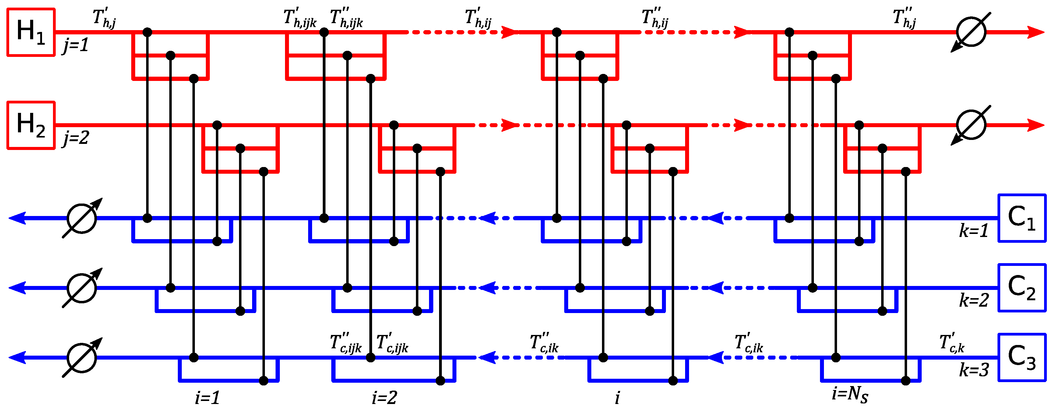
In order to represent different HEN solutions, a stage-wise superstructure proposed by Yee et al. [21] is used. As an example, a superstructure for two hot process streams $j$ and three cold process streams $k$ with stages $i$ is shown in Figure 1 including the nomenclature used in the following equations.

In each stage of the superstructure each hot stream is possibly connected with each cold stream. At the end of the streams a utility heat exchanger may be placed to ensure the desired target temperatures to get reached. Within the superstructure every heat exchanger has a specific index $ijk$ depending on the positioning:

$$ijk=\left(i-1\right)·N_h·N_c+\left(j-1\right)·N_c+k$$

(6)

Rearranging Equations (1)–(5) according to the outlet temperatures leads to a formulation which allows for the numerical calculation of the HEN temperatures:

$$\left[\begin{array}{c}{T}_{h,ijk}^{″}\\ T_{c,ijk}^{″}\end{array}\right]=\left[\begin{array}{cc}\frac{\left(1-R_{h,ijk}\right)e^{-NT{U}_{ijk}\left(1-R_{h,ijk}\right)}}{1-R_{h,ijk}{e}^{-NT{U}_{ijk}\left(1-R_{h,ijk}\right)}}\hfill & \frac{1-e^{-NT{U}_{ijk}\left(1-R_{h,ijk}\right)}}{1-R_{h,ijk}{e}^{-NT{U}_{ijk}\left(1-R_{h,ijk}\right)}}\hfill \\ \frac{R_{h,ijk}\left(1-e^{-NT{U}_{ijk}\left(1-R_{h,ijk}\right)}\right)}{1-R_{h,ijk}{e}^{-NT{U}_{ijk}\left(1-R_{h,ijk}\right)}}\hfill & \frac{1-R_{h,ijk}}{1-R_{h,ijk}{e}^{-NT{U}_{ijk}\left(1-R_{h,ijk}\right)}}\hfill \end{array}\right]\left[\begin{array}{c}{T}_{h,ijk}^{\prime }\\ T_{c,ijk}^{\prime }\end{array}\right]$$

(7)

with $R_{h,ijk}$ being:

$$R_{h,ijk}=\frac{{\dot{W}}_{h,ijk}}{{\dot{W}}_{c,ijk}}$$

(8)

and:

$$NT{U}_{ijk}=\frac{{\left(UA\right)}_{ijk}}{{\dot{W}}_{h,ijk}}$$

(9)

The corresponding non-isothermal mixing temperature for each process stream after each stage is calculated based on an energy balance [22]. The maximum number of stages to represent a HEN during optimization is set to $N_s=max\left\{N_h,N_c\right\}$ [22].

2.2. Objective Function

The objective function is structured in such way that a flexible cost functions framework can get incorporated in order to consider different implementation related factors like piping and pumping. A different cost function for every coupling of possible hot and cold process stream matches can be defined. In addition, different cost functions can get added for each utility heat exchanger. If necessary they can be further refined for every stage in the superstructure representation of the HEN. The objective function is based on the proposed structure by Rathjens and Fieg [1] and was further developed for the present work:

$$\begin{gathered} min\left\{{\displaystyle \sum }_{n=1}^{N_h+N_c}\left[C_{CU}·max\left\{{\dot{W}}_n\left(T_n^{″}-T_{out,n}^{+}\right),0\right\}+C_{HU}· max\left\{{\dot{W}}_n\left(T_{out,n}^{-}-T_n^{″}\right),0\right\}\right] \\ +{\displaystyle \sum }_{i=1}^{N_s}{\displaystyle \sum }_{j=1}^{N_h}{\displaystyle \sum }_{k=1}^{N_c}{z}_{ijk}{X}_{ijk}+{\displaystyle \sum }_{n=1}^{N_h+N_c}\left[z_{CU,n}{X}_{CU,n}+z_{HU,n}{X}_{HU,n}\right]\right\} \end{gathered}$$

(10)

Hot utility and cold utility are used to reach the desired target outlet temperatures $T_{out,n}$ and cause costs based on their individual supply costs $C_{HU}$ and $C_{CU}$. During optimization hot and cold utility can potentially be applied to each process stream depending on the maximum positive or negative deviation from the specified bounds of target temperatures. The respective utility which remains unused will make no contribution to the total annual costs (TAC). The binary variables $z$ state the existence of a heat exchanger within the superstructure. The match-based costs $X$ are calculated based on different cost function formulations with a wide range of possible correlations that can get implemented. The common cases of using a power function with the coefficients $a_0$, $a_1$ and $a_2$ as well as a general polynomial representation up to 4th degree (coefficients $b_0$, $b_1$, $b_2$, $b_3$ and $b_4$) are included. More specialized dependencies are covered using exponential (coefficients $c_0$ and $c_1$) or logarithmic expressions (coefficients $d_0$ and $d_1$):

$$X_{ijk}=\begin{array}{l}{a}_{0,ijk}+a_{1,ijk}{\xi }^{a_{2,ijk}}+\hfill \\ b_{0,ijk}+b_{1,ijk}\xi +b_{2,ijk}{\xi }^2+b_{3,ijk}{\xi }^3+b_{4,ijk}{\xi }^4\hfill \\ c_{0,ijk}+e^{c_{1,ijk}\xi }+\hfill \\ d_{0,ijk}\ln \left(\xi \right)+d_{1,ijk}\hfill \end{array}$$

(11)

The different cost function formulations given in Equation (11) are chosen because they were able to represent the cost correlations for practical implementation that were faced when working together with our industrial partners. In order to be used in the objective function, the dependencies given in Equation (11) have to get expressed through the individual heat exchanger areas $A$, the temperature levels $T$ and heat capacity flow rates $\dot{W}$ of the involved streams and the heat load $\dot{Q}$:

$$\xi ϵ\left\{A_{ijk},{\dot{W}}_{h,ijk},{\dot{W}}_{c,ijk},min\left\{{\dot{W}}_{h,ijk},{\dot{W}}_{c,ijk}\right\},max\left\{{\dot{W}}_{h,ijk},{\dot{W}}_{c,ijk}\right\},T_{h,ijk}^{\prime },T_{c,ijk}^{\prime },T_{h,ijk}^{″},T_{c,ijk}^{″},{\dot{Q}}_{ijk}\right\}$$

(12)

The expression of cost dependencies through distinct variables was chosen due to ensuring the universal applicability of the shown approach without extending the programming work for each different problem. Furthermore these variables can be used with minimal computational overhead. Because $\xi$ can be chosen out of an amount of alternatives given in Equation (12) the combinatorial possibilities of representing different cost dependencies are immense. The costs of utility heat exchangers $X_{HU,n}$ and $X_{CU,n}$ are structured equivalently to $X_{ijk}$.

2.3. Genetic Algorithm

The genetic algorithm uses the common genetic operations like selection, crossover and mutation. As optimization variables the parameters ${\left(UA\right)}_{ijk}$, ${\dot{W}}_{h,ijk}$ and ${\dot{W}}_{c,ijk}$ are used like proposed by Fieg et al. [22]. The selection is based on the fitness value $F$. The fitness value represents the quality of an individual with respect to the objective function. It is based on the relative relation towards the average costs among all individuals and the minimum TAC of all individuals. The calculation of the fitness value is given in the following equation:

$$F=\frac{C_{TAC}^{-1}+C_{TAC,min}^{-1}-2C_{TAC,avg}^{-1}}{C_{TAC,min}^{-1}-C_{TAC,avg}^{-1}}$$

(13)

The selection is carried out according to roulette wheel selection. Crossover is split in parameter crossover and structure crossover. Mutation is carried out on the variable parameters stated above. For details about the explicit formulations please refer to Fieg et al. [22]. The probability for the application of a crossover operation is 89% in this work and the probability for parameter crossover was chosen as 23% according to Brandt [23]. The probability for the general mutation is 1%, for parameter mutation it is 50% with a respective gene mutation probability of 1% [23].

Because of the optimization of the parameter ${\left(UA\right)}_{ijk}$ using the explicit temperature solution depicted in Equation (7) instead of the heat loads of the heat exchangers, every solution is thermodynamically feasible. Otherwise occurring temperature or heat load constraints can be omitted. The binary variable handling and corresponding constraints considering the continuous variables are adopted from Luo et al. [20]. During optimization the strategy of excessive use of utilities is used [24]. If the specified hot utility temperature is higher than any target temperature of all process streams and cold utility temperature is lower than any cold target temperature of all process streams, each network generated throughout optimization is feasible. As a result no outlet temperature constraints are considered here. Because ${\dot{W}}_{h,ijk}$ and ${\dot{W}}_{c,ijk}$ are also used as optimization variables, these values have to get constrained to be within a feasible region to hold the constraints given in Equations (14) and (15):

$${\displaystyle \sum }_{k=1}^{N_c}{\dot{W}}_{h,ijk}={\dot{W}}_{h,j}$$

(14)

$${\displaystyle \sum }_{j=1}^{N_h}{\dot{W}}_{c,ijk}={\dot{W}}_{c,k}$$

(15)

During optimization ${\dot{W}}_{h,ijk}^{*}$ and ${\dot{W}}_{c,ijk}^{*}$ can occur that violate the above mentioned constraints. In order to keep these constraints, the normalization strategy from Fieg et al. is applied [22], which is shown by the following equations:

$${\dot{W}}_{h,ijk}=\frac{{\dot{W}}_{h,j}}{{{\displaystyle \sum }}_{k=1}^{N_c}{\dot{W}}_{h,ijk}^{*}}{\dot{W}}_{h,ijk}^{*}$$

(16)

$${\dot{W}}_{c,ijk}=\frac{{\dot{W}}_{c,k}}{{{\displaystyle \sum }}_{j=1}^{N_h}{\dot{W}}_{c,ijk}^{*}}{\dot{W}}_{c,ijk}^{*}$$

(17)

Furthermore, the structural control strategy proposed by Luo et al. [20] was adapted to ensure heterogeneity in the population and avoid local optimal solutions.

Structurally forbidden matches are removed automatically from a possible occurrence in the superstructure by setting the respective ${\left(UA\right)}_{ijk}$ to zero. A simple assignment of high costs for the specific match is not efficient against the background of fast convergence. This is particularly true for the second example shown below.

2.4. Local Optimization

Due to the strong nonlinearity of the stated objective function, an algorithm relying only on genetic operations would take too long to find an acceptable solution. Therefore, deterministic methods are used for local optimization. In order to generate promising HEN structures in the initialization step the approach of enhanced vertical heat transfer proposed by Stegner et al. [25] is used. The method proposed by Stegner et al. [25] adopts ideas known from the conventional vertical heat transfer concepts from traditional pinch approach but a new form of graphic depiction was implemented. Loop breaking as one of the heuristic approaches known from pinch technology is considered as well. This approach was successfully combined with stochastic optimization by Brandt et al. [26].

Furthermore, Newton’s method is utilized for local parameter optimization [22]. Equation (18) shows the nomenclature in Newton’s method for the variables ${\left(UA\right)}_{ijk}^{*}$, ${\dot{W}}_{h,ijk}^{*}$ and ${\dot{W}}_{c,ijk}^{*}$ to get the optimized expression:

$$\left\{{\left(UA\right)}_{ijk},{\dot{W}}_{h,ijk},{\dot{W}}_{c,ijk}\right\}=\left\{{\left(UA\right)}_{ijk}^{*},{\dot{W}}_{h,ijk}^{*},{\dot{W}}_{c,ijk}^{*}\right\}-\frac{\raisebox{1ex}{$\partial C_{TAC}$}\!\left/ \!\raisebox{-1ex}{$\partial \left\{{\left(UA\right)}_{ijk}^{*},{\dot{W}}_{h,ijk}^{*},{\dot{W}}_{c,ijk}^{*}\right\}$}\right.}{\raisebox{1ex}{${\partial }^2{C}_{TAC}$}\!\left/ \!\raisebox{-1ex}{$\partial {\left\{{\left(UA\right)}_{ijk}^{*},{\dot{W}}_{h,ijk}^{*},{\dot{W}}_{c,ijk}^{*}\right\}}^2$}\right.}$$

(18)

The partial derivatives needed in Equation (18) are calculated numerically using a step size of 10⁻⁴.

3. Examples and Results

In order to show the application of the presented approach two examples have been chosen. Example 1 is a mid-sized optimization problem for direct heat integration. Example 2 is an optimization problem for indirect heat integration using a heat recovery loop (HRL).

3.1. Example 1

Example 1 was first stated by Pho and Lapidus [27] and was named 10SP1. It consists of five hot and five cold streams. In the first part of the analysis in our work we focus on the cost functions already used in other publications to achieve comparable results (see Section 3.1.1). In the second part we focus on additional costs caused by the consideration of piping (see Section 3.1.2).

3.1.1. Example 1a

The 10SP1 problem is well studied and has been used as an optimization case several times so far with decreasing costs throughout the years by many researchers (e.g., Nishida et al. [28] or Flower and Linnhoff [29].

During the last two decades the 10SP1 problem has still attracted a considerable amount of attention. The associated problem data is given in

Table 1. Problem data for example 1a.

Stream	${\mathit{T}}^{\prime }(°\mathbf{C})$	${\mathit{T}}_{\mathit{o}\mathit{u}\mathit{t}}(°\mathbf{C})$	$\mathit{h}$ ((kW/(m2K)	$\dot{\mathit{W}}$ (kW/K)	${\mathit{C}}_{\mathit{U}}$ ($/(kWyr))
H1	160	93	1.704	8.79	-
H2	249	138	1.704	10.55	-
H3	227	66	1.704	14.77	-
H4	271	149	1.704	12.56	-
H5	199	66	1.704	17.73	-
C1	60	160	1.704	7.62	-
C2	116	222	1.704	6.08	-
C3	38	221	1.704	8.44	-
C4	82	177	1.704	17.28	-
C5	93	205	1.704	13.90	-
HU	236	236	3.408	-	37.64
CU	38	82	1.704	-	18.12

. Two different formulations for the cost calculation of the annual costs of heat exchangers for the 10SP1 problem are given in the literature. The first cost formulation is given in Equation (19):

$$X_{ijk/H{U}_n/C{U}_n}=140·A_{ijk/H{U}_n/C{U}_n}^{0.6}$$

(19)

The second cost formulation is given in Equation (20):

$$X_{ijk/H{U}_n/C{U}_n}=145.63·A_{ijk/H{U}_n/C{U}_n}^{0.6}$$

(20)

A summary of the achieved TAC is given in

Table 2. Results comparison for example 1a.

Sources	Reported TAC ($/yr)
	Cost Formulation 1	Cost Formulation 2
Lewin et al. 1998 [24]	-	43,452 1 (43,752 1,3)
Lewin 1998 [30]	-	43,799 1
Lin and Miller 2004 [31]	43,329 2	-
Pariyani et al. 2006 [32]	-	43,439 1 (43,611 2)
Yerramsetty and Murty 2008 [34]	-	43,538 1
Peng and Cui 2015 [35]	-	43,411 1
Aguitoni et al. 2018 [36]	43,227 2	43,596 2
This work	42,963 2	43,321 2

¹ Solution without stream splits. ² Solution with stream splits. ³ Revised by Pariyani et al. [32].

. Several different approaches were used to tackle the 10SP1 problem. Lewin et al. [24] used a two-level approach consisting of a genetic algorithm and a lower level transformation into a linear parametric optimization problem. Lewin [30] also used an alternative nonlinear programming approach for the lower level optimization. Lin and Miller [31] used a tabu search algorithm to tackle the 10SP1 problem. Pariyani et al. [32] used a randomized algorithm for problems with stream splitting and a modified version of a previous work from Chakraborty and Ghosh [33] for designing networks without stream splitting. Yerramsetty and Murty [34] used a differential evolution algorithm and Peng and Cui [35] utilized a two-level simulated annealing algorithm. The latest work of Aguitoni et al. [36] found the best solution for the cost formulation 1 with a combination of a genetic algorithm and differential evolution.

The optimization procedure with the chosen approach incorporates 375 optimization variables considering five hot streams, five cold streams and five stages for the superstructure. Each heat exchanger has the same area-related cost function.

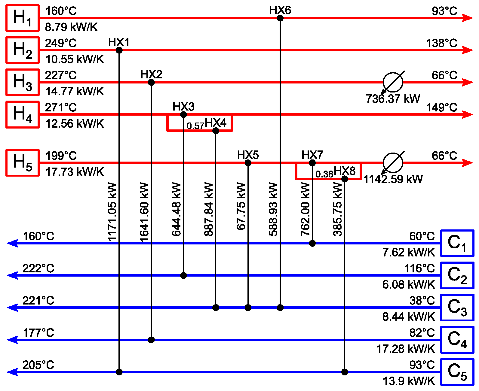
In our work cost formulation 1 was used for the optimization. The minimum TAC found was 42,963 $/yr. The solution is depicted in Figure 2 and shows a configuration of two stream splits as well as the use of two utility heat exchangers.

The cost formulation for the optimization is favoring maximum energy recovery (MER) networks. Therefore, the obtained network recovers the maximum amount of energy and only cold utility is used. The TAC obtained for example 1a is significantly lower than in the publications cited in relation to the progress in TAC made over the years. The HEN shown in Figure 2 was also evaluated using cost formulation 2 and the resulting costs are 43,321 $/a, which is the lowest TAC found for formulation 2 so far. The results show that the chosen approach is capable of generating competitive results compared to other approaches presented in literature. Therefore, the consideration of even more complex problem formulations should be manageable, which is shown in the following parts.

3.1.2. Example 1b

Example 1b is built on the problem definition from example 1a. In addition, piping costs are considered. The required coordinates for the corresponding streams are taken from Pouransari and Maréchal [18]. They added arbitrary Cartesian coordinates to the 10SP1 problem stated above. For the hot utility coordinates the values from Rathjens and Fieg [1] are used. The additional data is given in

Table 3. Additional Cartesian coordinates for the 10SP1 problem.

Stream	$\mathit{x}$ (m)	$\mathit{y}$ (m)	$\mathit{z}$ (m)
H1	4	3	8
H2	6	7	4
H3	9	8	7
H4	2	2	5
H5	2	8	2
C1	7	4	1
C2	9	3	10
C3	1	4	2
C4	8	6	9
C5	4	5	3
HU	5	5	0
CU	6	9	5

.

The required inner pipe diameter $D_i$ in m for each possible connecting pipe between a heat source and heat sink is calculated with the correlation for optimal diameter given by Peters et al. [37] for turbulent flow and $D_i\ge 0.0254$ m:

$$D_i=0.363·{\dot{V}}^{0.45}{\varrho }^{0.13}$$

(21)

with the volumetric flow rate $\dot{V}$ in m³/s, the fluid density $\varrho$ of 983 kg/m³ and a specific heat capacity of 4.18 kJ/(kgK).

Peters et al. [37] give a diagram for the correlation between pipe diameter and the related costs per meter of pipe. Due to manually selecting and reading out values from this diagram there might be a slight deviation from the book values which cannot be further specified. Considering stainless-steel welded pipe of type 304 [37] results in the following cost correlations with respect to the stream heat capacity flow rates and heat exchanger areas:

$$\begin{array}{cc}\hfill X_{ijk}=& 140·A_{ijk}^{0.6}+L_{jk}·\hfill \\ & \left(-0.174·{\left(min\left\{{\dot{W}}_{h,ijk},{\dot{W}}_{c,ijk}\right\}\right)}^2+17.773·\left(min\left\{{\dot{W}}_{h,ijk},{\dot{W}}_{c,ijk}\right\}\right)+27.426\right)\hfill \end{array}$$

(22)

and:

$$X_{C{U}_n}=140·A_{C{U}_n}^{0.6}+L_{C{U}_n,j}\left(-0.174·{\dot{W}}_{C{U}_n}^2+17.773·W_{C{U}_n}+27.426\right)$$

(23)

with the distance $L$ being:

$$L_{jk/C{U}_n,j}=2·\left(\left|x_j-x_{k/C{U}_n}\right|+\left|y_j-y_{k/C{U}_n}\right|+\left|z_j-z_{k/C{U}_n}\right|\right)$$

(24)

The number of optimization variables is 375 as in example 1a. However, the number of potentially different cost functions is 25 (each match between hot and cold stream). The number of potentially different cost functions for the hot and cold utility usage is 10 for each utility. The real number of different cost functions is lower due to the fact that some distances between multiple hot and cold streams as well as utilities are equal.

The relatively short distances between the heat sources and heat sinks are compensated by the annualization of the piping costs over a one-year period. As a result the portion of piping costs becomes around 35% of TAC.

The solution with the lowest TAC found in this work is shown in Figure 3a. It has a TAC of 68,476 $/yr. A structurally different solution which was found during optimization with a less complex structure but the same utility configuration is shown in Figure 3b.

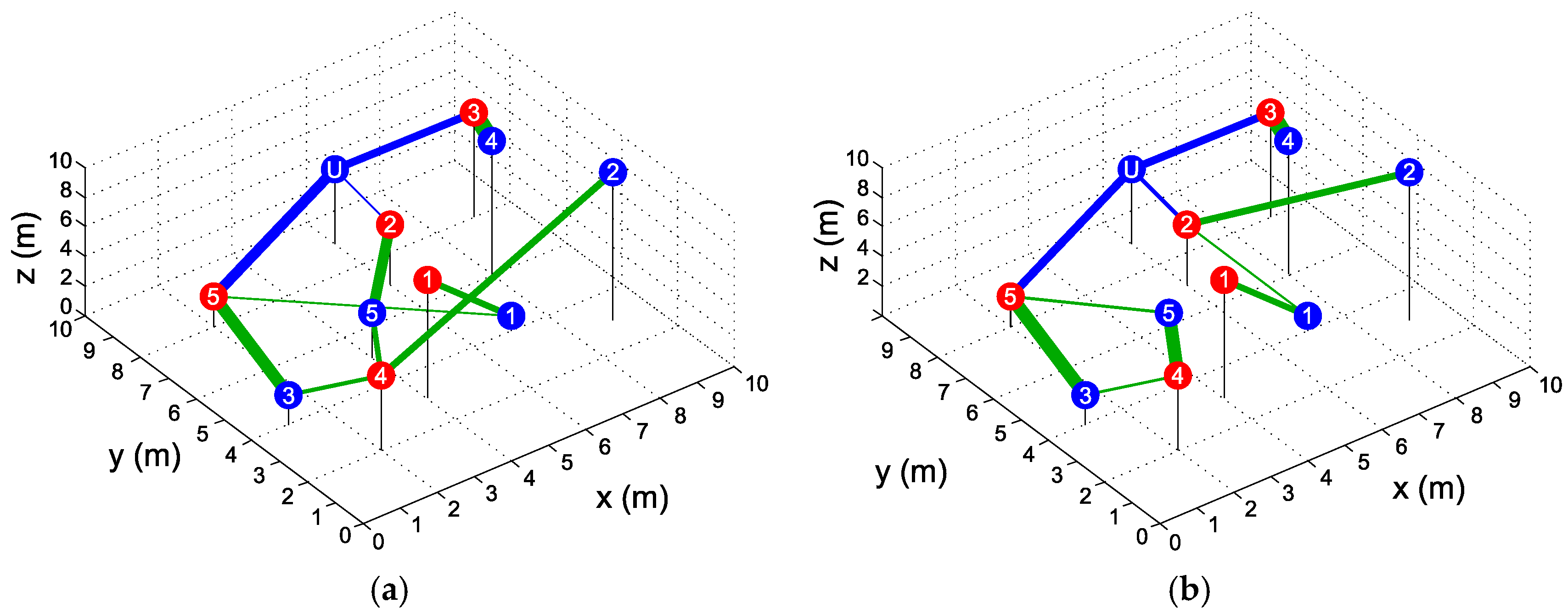
As opposed to the solution of example 1a only two stages within the superstructure are taken by heat exchangers. Furthermore, the number of utility heat exchangers increased to three compared to the case not considering piping. The results still represent MER networks. Figure 4 and Figure 5 show the relative orientation of the heat sources and heat sinks towards each other.

The configuration containing three utilities was dominant throughout the optimizations. The consideration of piping costs and thus the changed objective function had a strong influence on the heat load distribution within the HENs. The comparison between the optimal results of example 1b and example 1a shows about 14.2% (4016 $/yr) less piping costs, which is counterbalanced by an increase in installed heat exchanger area of about 16.2% (39.4 m²) and thus an increase in capital costs for the heat exchangers of 14.7% (1307 $/yr).

The favorable design of using cold utility for the streams H3 and H5 is still preferred when considering piping costs during optimization due to the coordinates chosen by Pouransari and Maréchal [18]. Furthermore the optimization is dominated by the close arrangement of the streams H3 and C4 as well as the streams H4, H5 and C3. Despite that, the solutions found considering piping costs already during the optimization are structurally different. Rathjens and Fieg [1] used a different cost functions formulation and were able to show significantly more local clustering of heat exchange similar to Figure 5b.

3.2. Example 2

The second example is a heat integration case with indirect heat integration utilizing a HRL with an intermediate fluid. It was taken from Chang et al. [13]. It is a case study of a heat integration project in the southern part of China. The example comprises two different plants with a distance $L$ of 1000 m. One plant is the heat source plant and the other one the heat sink plant with seven process streams each. The problem data is given in

Table 4. Problem data for example 2.

Stream	${\mathit{T}}^{\prime }(°\mathbf{C})$	${\mathit{T}}_{\mathit{o}\mathit{u}\mathit{t}}(°\mathbf{C})$	$\mathit{h}$ ((kW/(m2K)	$\dot{\mathit{W}}$ (kW/K)
H1 (plant1)	148.1	114.7	1.642	311.9
H2 (plant1)	145.4	105.6	1.451	303.3
H3 (plant1)	141.9	98.4	1.754	302.6
H4 (plant1)	140.8	75.5	1.411	307.4
H5 (plant1)	135.3	55.3	1.531	335.4
H6 (plant1)	133.9	42.2	1.721	330.2
H7 (plant1)	131.9	41.2	1.713	331.3
C1 (plant2)	78.2	135.7	1.518	335.4
C2 (plant2)	69.3	108.5	1.631	323.3
C3 (plant2)	60.5	95.6	1.108	305.6
C4 (plant2)	59.5	90.3	1.501	321.5
C5 (plant2)	50.2	79.5	1.203	381.5
C6 (plant2)	45.9	71.4	1.102	311.5
C7 (plant2)	42.9	65.4	1.102	301.5

$C_{HU}$ = 20 $/(kWyr), $C_{CU}$ = 8 $/(kWyr) [38]; $C_{HX}=\mathrm{11,000}+150·A_{HX}$ [39].

.

In addition to the utility costs and the capital costs for the heat exchangers, the costs for pumping and piping are considered. The detailed equations are given in the following part.

For the calculation of the inner pipe diameter $D_i$ for the HRL, Equation (21) is used. The fluid density of 960 kg/m³ and a specific heat capacity flow rate of 4.2 kJ/(kgK) is assumed.

The outer diameter $D_{out}$ in m, the specific pipe weight ${wt}_{pipe}$ in kg/m and the resulting pipe capital costs $Pcul$ in $/m for schedule 80 steel pipes are calculated according to Stijepovic and Linke [39]:

$$D_{out}=1.101·D_{in}+0.006349$$

(25)

$$w{t}_{pipe}=1330·D_{in}^2+75.18·D_{in}+0.9268$$

(26)

$$Pcul=0.82·w{t}_{pipe}+185D_{out}^{0.48}+6.8+295·D_{out}$$

(27)

The resulting capital costs for piping in $ are:

$$C_{pipe}=2·L·P_{cul}$$

(28)

For the calculation of the pumping capital costs the fanning friction factor $f$, the Reynolds number $Re$ and the fluid velocity $u$ in m/s are used to estimate the pressure drop $\mathsf{\Delta }p$ in Pa and the resulting costs [13,39]. The fluid velocity is calculated according to Equation (29) using the fluids mass flow rate $\dot{m}$ in kg/s of the intermediate fluid:

$$u=\frac{4·\dot{m}}{\varrho ·\pi ·D_{in}^2}$$

(29)

The Reynolds number is calculated assuming a dynamic viscosity $\mu$ of 0.0002834 Pa s:

$$Re=\frac{\varrho ·u·D_{in}}{\mu }$$

(30)

The resulting pressure drop $\mathsf{\Delta }p$ is given by:

$$\mathsf{\Delta }p=4·f·\frac{L·\varrho ·u^2}{2·D_{in}}$$

(31)

with the fanning friction factor of:

$$f=\frac{0.046}{R{e}^{0.2}}$$

(32)

The cumulated capital costs for the two pumps $C_{pump}$ in $ for the HRL are calculated according to Equation (33), utilizing the corresponding parameters for centrifugal pumps given in Jabbari et al. [40]:

$$C_{pump}=2·\left(8600+7310·{\left(\frac{\dot{m}·\mathsf{\Delta }p}{\varrho }\right)}^{0.2}\right)$$

(33)

The operating costs for pumping $C_{pump,op}$ in $/yr are composed of the pump efficiency ${\eta }_{pump}$ of 0.7, the price for electricity $C_{el}$ of 0.1 $/(kWh) [13], an operation duration $t$ of 8000 h/yr and the parameters calculated beforehand [13]:

$$C_{pump,op}=2·C_{el}·t·\frac{\dot{m}·\mathsf{\Delta }p}{\varrho ·{\eta }_{pump}}$$

(34)

The annualization of the capital costs for the heat exchangers, piping and the required pumps is done using an annualization factor $AF$ in 1/yr. The annualization factor is calculated according to Chang et al. [13] with an operation time $n$ of five years and a fractional interest rate $I$ of 10% per year:

$$AF=\frac{I·{\left(1+I\right)}^n}{{\left(1+I\right)}^n-1}$$

(35)

In order to use the superstructure of the utilized optimization model in this work, two pseudo-streams are added to the problem definition to emulate the HRL. The respective heat transfer coefficients for the two streams are 1 kW/(m²K) each [13,14]. The resulting superstructure has eight stages as well as eight hot streams and eight cold streams. In order to represent the cost correlations described beforehand, they are transferred to a dependency in heat capacity flow rate to get integrated in the cost functions framework proposed in this work. Therefore, the costs for piping and pumping are added up and calculated for different mass flow rates. The resulting costs are plotted against heat capacity flow rates calculated based on the respective mass flow rates. A curve fitting is carried out afterwards. The deviation from calculating the exact costs based on the equations given above is below 0.0012% considering rounded values for the piping and pumping costs. The resulting correlations are shown in Equation (36):

$$X_{ijk}=\{\begin{array}{cc}2910.77+39.57·{A_{ijk}}^1,\hfill & 2\le i\le 7,1\le j\le 7,k=1\hfill \\ (\mathrm{109,107.62}+300.52·{\dot{W}}_{h,j}-0.1019·{{\dot{W}}_{h,j}}^2\hfill & ijk=\left\{57,505\right\}\hfill \\ +3.7486·{10}^{-5}{{\dot{·W}}_{h,j}}^3-6.1293·{10}^{-9}{{\dot{·W}}_{h,j}}^4)/2,\hfill & \hfill \\ 2910.77+39.57·{A_{ijk}}^1,\hfill & 2\le i\le 7,j=8,2\le k\le 8\hfill \\ forbidden,\hfill & otherwise\hfill \end{array}$$

(36)

The utility heat exchangers for the two plants are considered as already installed like it was done by Chang et al. [13]. Therefore, $X_{HU,n}$ and $X_{CU,n}$ are zero for this example. The first and last stages are used to include the costs for pumping and piping. The areas of the heat exchangers to emulate the HRL ($ijk=\left\{57,505\right\}$) are chosen to be near infinite by the algorithm to avoid utility usage, thus create a self-adjusting temperature level and balance the heat transferred from the heat source plant to the heat sink plant. In order to prohibit direct heat integration between the two plants, all direct matches are forbidden. Altogether the applied superstructure yields 1536 optimization variables (compared to 1029 for direct heat integration without the pseudo streams). Due to the large number of forbidden matches (426) in relation to the number of possible matches (512), the number of optimization variables considered is reduced equivalently. The whole problem is described with only three different cost functions (see Equation (36)).

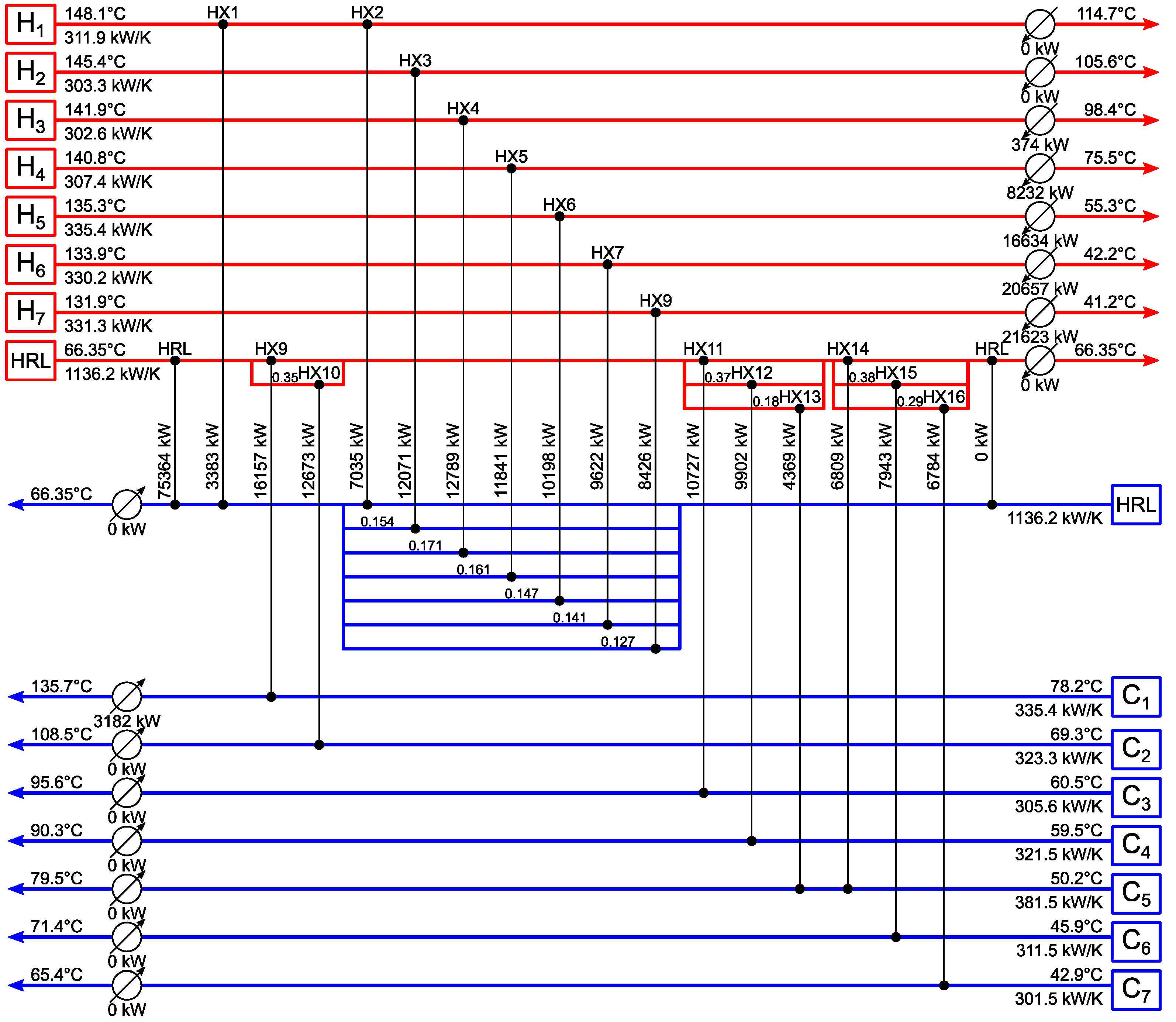
Iteration over the mass flow rate yields the optimal configuration for the HRL for example 2 which is shown in Figure 6. The superstructure representation of the solution in Figure 6 is shown in Figure A1 in Appendix A.

The TAC achieved for the solution shown in Figure 6 is 1.54 M$/yr. The associated annualized capital costs for the heat exchangers are 0.574 M$/yr (37.2% of TAC) and the utility consumption causes annual costs of 0.603 M$/yr (39.1% of TAC). The overall piping costs are 0.326 M$/yr (21.1% of TAC) and pumping costs are 0.038 M$/yr (2.5% of TAC). The solution obtained in this work is therefore 4.4% cheaper than the solution reported by Chang et al. [13]. These differences are explained by the non-isothermal mixing model used and the relaxed temperature constraints in this work.

4. Conclusions

The presented approach to incorporate a flexible cost functions framework to synthesize cost-optimal heat exchanger networks (HENs) was carried out successfully and showed promising results. The flexible structured objective function allows for the integration of individual, match-dependent cost functions. The introduction of pseudo streams in combination with the flexible cost functions framework allow for the application for various problems. Corresponding optimizations utilizing different parametrizations have been carried out successfully. The universal applicability was shown by the execution of optimizations with different areas of application. The presented approach is applicable for direct as well as indirect heat integration utilizing the same superstructure and the same genetic algorithm for solving the problems. The use for combined direct and indirect heat integration is possible if initially forbidden matches get extended with cost information. This work presents results with lower TAC than other results published in literature beforehand.

For the practical implementation it is advisable to incorporate factors like piping already during optimization. The consideration of these factors can have a huge impact of the overall HEN structure and can lead towards significantly different and more efficient solutions. Local clustering was observed for some solutions like already reported by Rathjens and Fieg [1].

References

- Rathjens, M.; Fieg, G. Design of cost-optimal heat exchanger networks considering individual, match-dependent cost functions. Chem. Eng. Tran. 2018, 70, 601–606. [Google Scholar] [CrossRef]
- Linnhoff, B.; Hindmarsh, E. The pinch design method for heat exchanger networks. Chem. Eng. Sci. 1983, 38, 745–763. [Google Scholar] [CrossRef]
- Papoulias, S.A.; Grossmann, I.E. A structural optimization approach in process synthesis—II. Heat recovery networks. Comput. Chem. Eng. 1983, 7, 707–721. [Google Scholar] [CrossRef]
- Klemeš, J.J.; Kravanja, Z. Forty years of Heat Integration: Pinch Analysis (PA) and Mathematical Programming (MP). Curr. Opin. Chem. Eng. 2013, 2, 461–474. [Google Scholar] [CrossRef]
- Dhole, V.R.; Linnhoff, B. Total site targets for fuel, co-generation, emissions, and cooling. Comput. Chem. Eng. 1993, 17, S101–S109. [Google Scholar] [CrossRef]
- Chew, K.H.; Klemeš, J.J.; Wan Alwi, S.R.; Abdul Manan, Z. Industrial implementation issues of Total Site Heat Integration. Appl. Therm. Eng. 2013, 61, 17–25. [Google Scholar] [CrossRef]
- Liu, X.; Klemeš, J.J.; Varbanov, P.S.; Qian, Y.; Yang, S.; Liu, X.; Varbanov, P.S.; Klemes, J.J.; Wan Alwi, S.R.; Yong, J.Y. Safety issues consideration for direct and indirect heat transfer on total sites. Chem. Eng. Trans. 2015, 45, 151–156. [Google Scholar] [CrossRef]
- Nemet, A.; Klemeš, J.J.; Moon, I.; Kravanja, Z. Safety Analysis Embedded in Heat Exchanger Network Synthesis. Comput. Chem. Eng. 2017, 107, 357–380. [Google Scholar] [CrossRef]
- Nemet, A.; Klemeš, J.J.; Kravanja, Z. Process synthesis with simultaneous consideration of inherent safety-inherent risk footprint. Front. Chem. Sci. Eng. 2018, 12, 745–762. [Google Scholar] [CrossRef]
- Escobar, M.; Trierweiler, J.O.; Grossmann, I.E. Simultaneous synthesis of heat exchanger networks with operability considerations: Flexibility and controllability. Comput. Chem. Eng. 2013, 55, 158–180. [Google Scholar] [CrossRef]
- Rathjens, M.; Bohnenstädt, T.; Fieg, G.; Engel, O. Synthesis of heat exchanger networks taking into account cost and dynamic considerations. Procedia Eng. 2016, 157, 341–348. [Google Scholar] [CrossRef]
- Pavão, L.V.; Miranda, C.B.; Costa, C.B.B.; Ravagnani, M.A.S.S. Efficient multiperiod heat exchanger network synthesis using a meta-heuristic approach. Energy 2018, 142, 356–372. [Google Scholar] [CrossRef]
- Chang, C.; Chen, X.; Wang, Y.; Feng, X. An efficient optimization algorithm for waste Heat Integration using a heat recovery loop between two plants. Appl. Therm. Eng. 2016, 105, 799–806. [Google Scholar] [CrossRef]
- Wang, Y.; Wang, W.; Feng, X. Heat integration across plants considering distance factor. Chem. Eng. Trans. 2013, 35, 25–30. [Google Scholar] [CrossRef]
- Wang, Y.; Chang, C.; Feng, X. A systematic framework for multi-plants Heat Integration combining Direct and Indirect Heat Integration methods. Energy 2015, 90, 56–67. [Google Scholar] [CrossRef]
- Chang, C.; Chen, X.; Wang, Y.; Feng, X. Simultaneous optimization of multi-plant heat integration using intermediate fluid circles. Energy 2017, 121, 306–317. [Google Scholar] [CrossRef]
- Liew, P.Y.; Wan Alwi, S.R.; Klemeš, J.J. Total Site Heat Integration Targeting Algorithm Incorporating Plant Layout Issues. In 24th European Symposium on Computer Aided Process Engineering; Klemes, J., Varbanov, P.S., Liew, P.Y., Eds.; Elsevier Science: Burlington, NJ, USA, 2014; pp. 1801–1806. [Google Scholar]
- Pouransari, N.; Maréchal, F. Heat exchanger network design of large-scale industrial site with layout inspired constraints. Comput. Chem. Eng. 2014, 71, 426–445. [Google Scholar] [CrossRef]
- Souza, R.D.; Khanam, S.; Mohanty, B. Synthesis of heat exchanger network considering pressure drop and layout of equipment exchanging heat. Energy 2016, 101, 484–495. [Google Scholar] [CrossRef]
- Luo, X.; Wen, Q.-Y.; Fieg, G. A hybrid genetic algorithm for synthesis of heat exchanger networks. Comput. Chem. Eng. 2009, 33, 1169–1181. [Google Scholar] [CrossRef]
- Yee, T.F.; Grossmann, I.E.; Kravanja, Z. Simultaneous optimization models for heat integration—I. Area and energy targeting and modeling of multi-stream exchangers. Comput. Chem. Eng. 1990, 14, 1151–1164. [Google Scholar] [CrossRef]
- Fieg, G.; Luo, X.; Jeżowski, J. A monogenetic algorithm for optimal design of large-scale heat exchanger networks. Chem. Eng. Process. Process Intensif. 2009, 48, 1506–1516. [Google Scholar] [CrossRef]
- Brandt, C. Entwicklung und Implementierung Eines Hybriden Genetischen Algorithmus für die Automatisierte Auslegung von Kostenoptimalen Wärmeübertragernetzwerken; Shaker: Herzogenrath, Germany, 2018. [Google Scholar]
- Lewin, D.R.; Wang, H.; Shalev, O. A generalized method for HEN synthesis using stochastic optimization—I. General framework and MER optimal synthesis. Comput. Chem. Eng. 1998, 22, 1503–1513. [Google Scholar] [CrossRef]
- Stegner, C.; Brandt, C.; Fieg, G. EVHE—A new method for the synthesis of HEN. Comput. Chem. Eng. 2014, 64, 95–102. [Google Scholar] [CrossRef]
- Brandt, C.; Fieg, G.; Luo, X. Efficient synthesis of heat exchanger networks combining heuristic approaches with a genetic algorithm. Heat Mass Transf. 2011, 47, 1019–1026. [Google Scholar] [CrossRef]
- Pho, T.K.; Lapidus, L. Topics in computer-aided design: Part II. Synthesis of optimal heat exchanger networks by tree searching algorithms. Aiche J. 1973, 19, 1182–1189. [Google Scholar] [CrossRef]
- Nishida, N.; Liu, Y.A.; Lapidus, L. Studies in chemical process design and synthesis: III. A Simple and practical approach to the optimal synthesis of heat exchanger networks. Aiche J. 1977, 23, 77–93. [Google Scholar] [CrossRef]
- Linnhoff, B.; Flower, J.R. Synthesis of heat exchanger networks: II. Evolutionary generation of networks with various criteria of optimality. Aiche J. 1978, 24, 642–654. [Google Scholar] [CrossRef]
- Lewin, D.R. A generalized method for HEN synthesis using stochastic optimization—II. The synthesis of cost-optimal networks. Comput. Chem. Eng. 1998, 22, 1387–1405. [Google Scholar] [CrossRef]
- Lin, B.; Miller, D.C. Solving heat exchanger network synthesis problems with Tabu Search. Comput. Chem. Eng. 2004, 28, 1451–1464. [Google Scholar] [CrossRef]
- Pariyani, A.; Gupta, A.; Ghosh, P. Design of heat exchanger networks using randomized algorithm. Comput. Chem. Eng. 2006, 30, 1046–1053. [Google Scholar] [CrossRef]
- Chakraborty, S.; Ghosh, P. Heat exchanger network synthesis: The possibility of randomization. Chem. Eng. J. 1999, 72, 209–216. [Google Scholar] [CrossRef]
- Yerramsetty, K.M.; Murty, C.V.S. Synthesis of cost-optimal heat exchanger networks using differential evolution. Comput. Chem. Eng. 2008, 32, 1861–1876. [Google Scholar] [CrossRef]
- Peng, F.; Cui, G. Efficient simultaneous synthesis for heat exchanger network with simulated annealing algorithm. Appl. Therm. Eng. 2015, 78, 136–149. [Google Scholar] [CrossRef]
- Aguitoni, M.C.; Pavão, L.V.; Siqueira, P.H.; Jiménez, L.; Ravagnani, M.A.S.S. Synthesis of a cost-optimal heat exchanger network using genetic algorithm and differential evolution. Chem. Eng. Trans. 2018, 70, 979–984. [Google Scholar] [CrossRef]
- Peters, M.S.; Timmerhaus, K.D.; West, R.E. Plant Design and Economics for Chemical Engineers, 5th ed.; McGraw-Hill: Boston, MA, USA, 2003. [Google Scholar]
- Hipólito-Valencia, B.J.; Rubio-Castro, E.; Ponce-Ortega, J.M.; Serna-González, M.; Nápoles-Rivera, F.; El-Halwagi, M.M. Optimal design of inter-plant waste energy integration. App. Therm. Eng. 2014, 62, 633–652. [Google Scholar] [CrossRef]
- Stijepovic, M.Z.; Linke, P. Optimal waste heat recovery and reuse in industrial zones. Energy 2011. [Google Scholar] [CrossRef]
- Jabbari, B.; Tahouni, N.; Ataei, A.; Panjeshahi, M.H. Design and optimization of CCHP system incorporated into kraft process, using Pinch Analysis with pressure drop consideration. App. Therm. Eng. 2013, 61, 88–97. [Google Scholar] [CrossRef]
Figure 1.
Stage-wise superstructure of a heat exchanger network (HEN) with two hot and three cold process streams.
Figure 2.
Grid-diagram representation of the optimal HEN configuration of example 1a (TAC: 42,963 $/yr).
Figure 3.
Grid-diagram representations of: (a) the optimal HEN configuration of example 1b (TAC: 68,476 $/yr); and (b) an alternative HEN configuration of example 1b (TAC: 68,843 $/yr).
Figure 4.
(a) 3D layout representation of the optimal HEN configuration of example 1b, the chosen line thickness is proportional to the corresponding heat exchanger heat load; and (b) 3D layout representation of the alternative HEN configuration of example 1b, the chosen line thickness is proportional to the corresponding heat exchanger heat load.
Figure 5.
(a) 2D layout representation of the optimal HEN configuration of example 1b; (b) 2D layout representation of the alternative HEN configuration of example 1b.
Figure 6.
Plant representation of the optimal HEN configuration found of example 2 including a HRL (TAC: 1.54 M$/yr).