Analysis of the Design of a Poppet Valve by Transitory Simulation


1
Mechanical Engineering Department, Universidad de Los Andes, Bogota 111711, Colombia
2
School of Engineering Technology, Purdue University, West Lafayette 47907, IN, USA
*
Author to whom correspondence should be addressed.
Energies 2019, 12(5), 889; https://doi.org/10.3390/en12050889
Submission received: 10 February 2019
/
Revised: 27 February 2019
/
Accepted: 2 March 2019
/
Published: 7 March 2019
(This article belongs to the Special Issue Energy Efficiency and Controllability of Fluid Power Systems 2018)
Abstract
:This article contains the results and analysis of the dynamic behavior of a poppet valve through CFD simulation. A computational model based on the finite volume method was developed to characterize the flow at the interior of the valve while it is moving. The model was validated using published data from the valve manufacturer. This data was in accordance with the experimental model. The model was used to predict the behavior of the device as it is operated at high frequencies. Non-dimensional parameters for generalizing and analyzing the effects of the properties of the fluid were used. It was found that it is possible to enhance the dynamic behavior of the valve by altering the viscosity of the working fluid. Finally, using the generated model, the influence of the angle of the poppet was analyzed. It was found that angle has a minimal effect on pressure. However, flow forces increase as angle decreases. Therefore, reducing poppet angle is undesirable because it increases power requirements for valve actuation.
1. Introduction
An Electro hydraulic Servo Valve (EHSV) is a directional valve capable of accurately and proportionally metering flow based on a given input. These valves have been used extensively in aerospace applications since the 1950s particularly for flight control surfaces and other secondary functions. Other typical applications include power steering actuators and in electronically controlled industrial applications [1]. These valves are favored because they can be used to implement excellent feedback control systems while operating with relatively low power.
In recent years model based diagnostics and prevention has been investigated to improve the reliability of Electro-hydraulic, Electro-mechanical and Electro-pneumatic systems [2,3,4,5,6,7]. In typical EHSV’s the radial clearance between the spool and the sleeve in the valves is in the order of 5 µm or 0.2 thousand of an inch [8]. This tight gap tends to break the fluid and form sticky films increasing viscous friction and eventually creating spool stiction. Finally, from a hydraulics perspective, systems operating with EHSV tend to be inherently energy inefficient because they restrict the flow passing from the supply port to the work port through metered orifices. This restriction creates a pressure drop that is converted into heat [9,10]. The heated fluid can vaporize at low pressure, increasing the possibility of cavitation in standard applications.
Possible solutions to replace the traditional 4/3 directional controlled valve used in hydraulic systems to control the motion of an actuator include: (1) Displacement control actuation [11,12], (2) independent metering control [13,14], and (3) digital hydraulics [15,16,17,18]. Each of these solutions has its own strengths and weaknesses. While the first approach is great for controllability, stability, and efficiency, its implementation is costly because it requires a single pump for each actuator. Solution (2), improves energy efficiency significantly but still uses valves with spools that are also sensitive to contamination. Solution (3) uses poppet on-off valves (valves with only two positions), which are resilient against contamination, are relatively inexpensive and easy to operate. However, on-off poppet valves lack the speed of EHSV and the implementation of control strategies to achieve closed loop control of an actuator can be challenging. Solenoid operated poppet valves have been implemented in a great variety of applications. Thanks to their low cost and simple operation, these valves have replaced other technologies. For instance, the use of poppet style valves has been introduced in the automotive market replacing traditional cam-lever designs for controlling intake and exhaust in diesel engines [19]. Multiple solenoid poppet valves can be connected in parallel to construct a digital flow control unit (DFCU) to replicate the operation of an EHSV, with similar or better flow capacities and in theory better controllability, optimized energy consumption and significantly lower cost. With the purpose of replacing an EHSV for a group of DFCU’s, various researchers have focused on improving the resolution and controllability of an optimized number of valves [20]. One such control method is the implementation of Pulse Width Modulation (PWM) for controlling the flow using independent valves [21]. However, the typical high non-linearity of flow through an orifice in any valve still remains a great challenge. It has been proposed that a main issue of these non-linearities is their effect on response time of the valve being far greater than the control signal [22]. In other words, to improve the controllability issues due to non-linearities, it is necessary to increase the speed of the DFCU to obtain a comparable behavior to an EHSV. For poppet valves, the response time is always tied to the fluid flow forces, the slower the response time of the valve, the larger the flow forces acting on the poppet. One possible alternative to overcome these flow forces is to improve the electromagnetic properties of the solenoid operating the poppet valve. Some researchers have used solenoids with metal alloys like Al-Fe [19], Ti [20] or have resorted to the use of magneto-rheological fluids [23], with response times between 0.16 to 0.45 ms, 7–10 ms and 0.1–100 ms, respectively.
Another parameter of interest for improving the response time of a DFCU is the geometry of the poppet and the seat. Studies have focused on decreasing the flow forces through empirical and computational analysis to evaluate the effect of angle on spool valves. Flow forces seen in these studies were reduced by approximately 36% [24]. Others have optimized rotary spool valves using genetic algorithms, where the energetic performance of the valve was improved by up to a 97% [25]. Computational Fluid Dynamics (CFD) is generally used for modeling and approximating the Navier-Stokes Equations to characterize flow through a valve. CFD analysis performed on poppet valves has been used to predict the behavior of these valves with relative errors below 8% [26,27]. Nevertheless, it is important to note that is has also been demonstrated that errors are related to many factors, such as geometry and that some configurations are more challenging for the mathematical models [28]. It is for this reason it is important to perform careful mesh sensitivity analysis to assess the performance of the model. The goal of this study was to characterize the behavior of a commercial poppet valve in transient state using CFD, and to focus on its response at high frequencies by analyzing the flow forces, geometric characteristics and pressure gradients. The model was validated using the manufacturer’s published experimental data and subsequently used to study the effect of geometric changes on the velocity of the poppet to make PWM control easier to implement on DFCU valves.
2. Problem Definition
2.1. Computational Domain
The computational model was established starting with a commercial model of a solenoid controlled, 2 position and 3 port, poppet valve as seen in Figure 1. A computational domain to characterize the flow through ports 1 and 2 was developed. Port 3 was not completely modeled because the disregarded portion doesn’t significantly affect the flow in the head area and therefore it is considered negligible. The cartridge valve was assumed to be inserted into a manifold where each port is connected to pipes assumed to be long enough to consider fully developed flow. The length of the pipes was estimated using turbulent flow in pipe theory per Equation (1) and the properties of flow at the normal valve operating conditions. It was estimated that the pipe length should not be less than 0.13 m.
The geometric model of the poppet valve was simplified by not considering elements like the seals and retaining rings from the cartridge inserted in the manifold, as well as the fittings used to connect the tubbing to the manifold ports. These elements are assumed to have a negligible effect as was noted in previous studies [29,30]. The geometry of the implemented domain is shown in Figure 2, below.
2.2. Governing Equations
2.2.1. Conservation Equations
The mass and moment conservation Equations for incompressible flow excluding all external forces, including gravitational forces are given by the following Equations. It is assumed that changes in density of the fluid are very small and therefore negligible in the analysis.
and,
Assuming isentropic and Newtonian flow, the stress tensor is defined as:
2.2.2. RANS Models
The Reynolds-averaged Navier–Stokes (RANS) models are Equations of motion for fluid flow averaged over time and were used to model turbulence. The model assumes that an instantaneous quantity is decomposed into its time-averaged and fluctuating quantities.
The RANS Equations for the conservation Equations become:
where the term is known as the Reynolds stress. In this model the Boussinesq eddy viscosity assumption is used, and the Reynolds stress then becomes:
where is known as the turbulent viscosity or Eddy viscosity and is the average turbulent energy. The set of Equations (5)–(8) together with a turbulence model to solve for the turbulent viscosity are used to model the turbulent flow and were solved using a commercial CFD solver (ANSYS® Academic Research Fluent, Release 17).
2.2.3. Wall Effect Functions
Turbulent flows are significantly affected by the presence of walls where no slip occurs. This generates changes in the behavior of the turbulent flow and large velocity gradients, where generally speaking, linearized discretization methods do not appropriately match the real flow values. When using RANS models, particularly of the family of κ-ε models in this work, empirical functions known as wall effect functions may be implemented to account for the effects of this boundary layer. It is always necessary to develop a mesh with refined elements at and near the surface to satisfy boundary layer requirements. The level of refinement required depends upon both the turbulence model and the wall function being selected.
The standard wall effect function assumes a logarithmic profile to model effects of turbulent flow near a boundary.
where the terms k, E, C are empirical terms, and are non-dimensional terms for the velocity and the position of the boundary layer, respectively.
2.3. Numerical Methods
2.3.1. CFD Methods
For this project the simulations were performed using ANSYS® Academic Research Fluent, Release 17. In all simulated cases the model was initialized using potential flow, the SIMPLE algorithm was used for the solution of the conservation Equations and second-order discretization schemes for pressure, velocity and turbulent terms were used. Finally, transient simulations with a temporally implicit scheme were implemented for the dynamic analysis. Results from steady state simulations were used to initialize the model and the “layering” meshing technique was implemented for simulating the movement of the valve poppet within the mesh.
The constant pressure outlet boundary conditions were implemented at the Section next to port 3 and at the exit pipe. At the inlet of the pipe a fixed velocity was imposed for steady state simulations and a fixed pressure condition was imposed for the transient simulations to ensure mathematical stability. An interface boundary condition between the exit pipe and port 2 of the valve was implemented, where in case of mutual contact one side would act as an internal face and the other as a boundary wall, the implemented boundary conditions are shown in Figure 3.
2.3.2. Mesh Independence
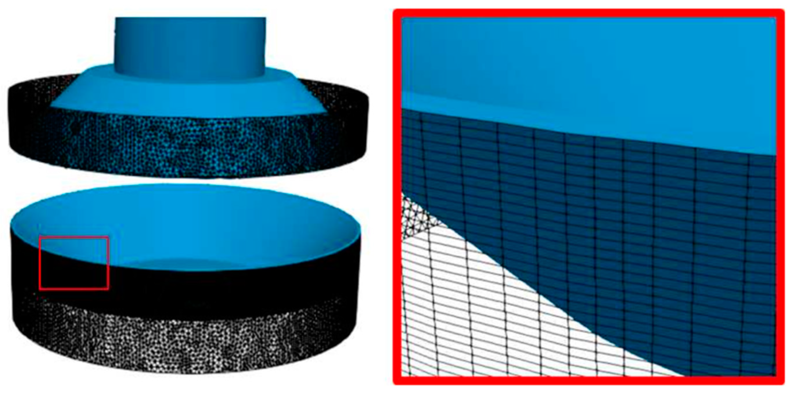
All meshes were generated using ANSYS® Academic Research ICEM, Release 17 software, the meshing method used is called “Octree” with prismatic elements generated for the walls at the inlet and outlet pipes. The mesh was refined at the valve, especially near the poppet and seat areas. The mesh was initially generated assuming ports 1 and 2 were closed, and the “layering” tool for generation of dynamic meshes of ANSYS® Academic Research Fluent, Release 17 was used to connect ports 1 and 2 according to the poppet dimensions as shown in Figure 4. The independence of the mesh was evaluated with 5 progressively refined meshes applied over the entire domain.
Mesh refinements were realized using approximately 20% increases in the number of elements between meshes. Simulations were evaluated at a velocity of 8.83 m/s, equivalent to approximately 4.44E-04 m3/s (7.04 gpm or 26.6 lpm), with fluid properties as listed in Table 1.
Mesh independence was tested using two thousand iterations of the steady state simulations where the residuals were verified to be less than 10−5. For this mesh independence study standard κ-ε was used. The poppet has the standard commercial geometry and the state of the valve is fully open allowing flow from port 1 to port 2. The convergence parameter selected was a pressure differential measured at 5 diameters downstream and 10 diameters upstream with respect to the valve in accordance with ISO standard ISO 4411:2008 [31].
The pressure differentials obtained with the simulations were compared to the reported values from Sun hydraulics manufacturer’s data-sheet for valve model DWDA. All valves are tested at the manufacturer’s facility using petroleum-based hydraulic fluid with a viscosity of approximately 25 cSt. and a 19/17/14 fluid cleanliness level per ISO 4406 [32]. Table 2 below presents a comparison between the published data and the corresponding simulated values.
Results with errors less than 7% were obtained using the three finer meshes, and based on these preliminary results, it was decided to use a mesh with approximately 9.8 million elements to ensure good resolution at a reasonable computational time in comparison to the mesh with 12.3 million of elements.
2.3.3. Turbulence Models
Similar to the process followed to test the mesh convergence, an evaluation process for validating the turbulence models and wall functions was used. The evaluated turbulence models were the Standard κ-ε, Realizable κ-ε, κ-ω SST and Spalart-Allmaras. Two wall functions were evaluated, mainly the Scalable Wall Functions (SWF) and Enhanced Wall Treatment (EWT) both available in the software. Various combinations of turbulence models and wall functions were tested for runs consisting of two thousand iterations of the steady state model and the pressure differentials obtained from the simulation were compared to that of the published results. Table 3 below lists the results obtained for the selection of the most appropriate turbulence and wall function combinations. The results had a relative error of less than 13% for all turbulence models. The Standard κ-ε turbulence model with EWT was selected because it had a lower relative error.
Given the results presented in Table 3 the combination for turbulence model and wall function of Standard κ-ε and EWT, respectively, is used in the rest of the work. For this flow rate an error of less than 1% was obtained with respect to the published pressure drop. This combination of models is able to accurately model the boundary layer and the viscous dissipation therein.
3. Results and Discussion
3.1. Results Validation using Manufacturer’s Published Data
Before proceeding to analyze the dynamic simulation results, the selected model was validated using the pressure differential at various flow rates. The simulations were developed in steady state with six thousand iterations obtaining residuals of magnitudes less than 10-6. These results are listed in Table 4 below and plotted in Figure 5. Notice that the slight difference between the pressure drop at the higher flow rate of Table 4 and that obtained in the previous Section (Table 3) is due to the results in this Section being obtained with six thousand iterations (two thousand in the previous Section). The simulated data demonstrates less than 5% error at flow rates of 2.24 × 10⁻⁴ m3/s (3.55 gpm or 13.4 lpm) and greater. The higher percentual error at lower flow rates is very likely due to the flow transitioning to laminar at this lower Reynolds numbers (approximately Re = 467 based on the diameter of the port for the lower flow rate) and the turbulence model struggling to accurately capture the physics of the system.
3.2. Dynamic Analysis
3.2.1. Results at a Frequency of 25 Hz
Starting from the good fitting of the simulation model and the manufacturer’s experimental data sheet, the movement of the valve in the dynamic analysis was modeled in three different ways. First, for the opening process where ports 1 and 2 are initially disconnected, the model was configured so that the displacement of the valve was represented by the function in Equation (10).
Equation (10) is a continuous approximation of the “head-viside” function, where A is the total motion amplitude of the valve with a magnitude of 2.501 mm, Kh is a constant value affecting the time required for the poppet to traverse from one position to the other, De is an induced valve delay for obtaining steady state data before the poppet starts moving. These values were selected to match the actual valve time of 40 ms required to move the poppet from the fully closed to fully open position. The configuration for the displacement of the poppet for opening and closing of the valve assumed it was the same function with an opposite sign. The control signal to operate the position of the poppet was assumed to follow a sinusoidal signal of the form:
The implemented movements of the poppet are displayed in Figure 6.
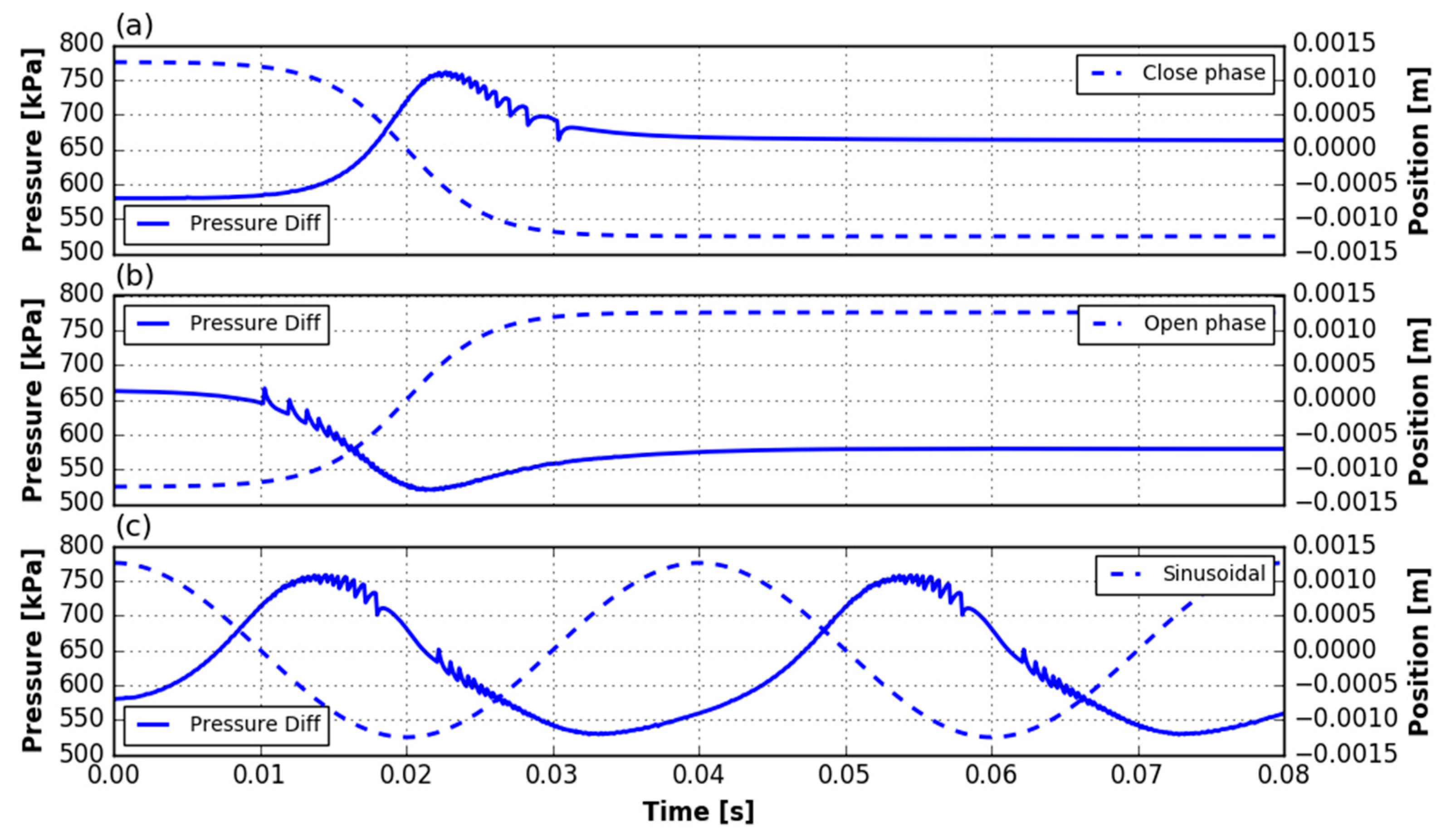
All the simulations were initialized with 6000 iterations in steady state at the initial position. Later the simulation was carried out in transient state with a simulation time of 0.08 ms and time steps of 0.001 ms and 30 iterations per time step. The simulations were evaluated using the optimal values obtained from the mesh independence study presented in Section 2.3.2., at approximately the same flow rate used in the study. The resulting inlet velocity was estimated to be 8.83 m/s and 666.4 kPa. The results of the dynamic analysis for opening and closing the valve are shown in Figure 7. It was found that pressure drop during the single opening and closing procedure is similar to the result obtained with a fluctuating sinusoidal position command. Approximate values of 500 and 760 kPa were observed as maximum and minimum pressure drops during valve opening and closing events. Small pressure instabilities during the opening and closing procedures were observed just after reaching the maximum position of the poppet while ports 1 and 2 were open. Changes to the time parameters De and Kh did not show a significant effect on reducing or increasing the instabilities. Also, varying the amount of iterations per time step didn’t have much effect in reducing the instabilities. Therefore, these instabilities might be associated to the remeshing algorithm during the opening and closing of the valve. Likewise, other authors have demonstrated that the force instability increases as the valve opening is small which might suggest that the instabilities are physical [33,34].
3.2.2. Parametric Analysis
The inlet pressure and input poppet frequency were changed to analyze the effect of these parameter on the behavior of the pressure drop, poppet force and flow for two cycles of poppet motion using a sinusoidal input. These simulations were conducted in order to understand the effect on pressure differential at various poppet frequencies as well as different flow inputs. The levels for each of the parameters used in the simulations are summarized in Table 5. The time steps in the simulations were adjusted so that at each step the poppet had achieved the same position irrespective of the input frequency. The flow rates selected were based on simulations obtained during the steady state validation of the mesh presented in Section 2.
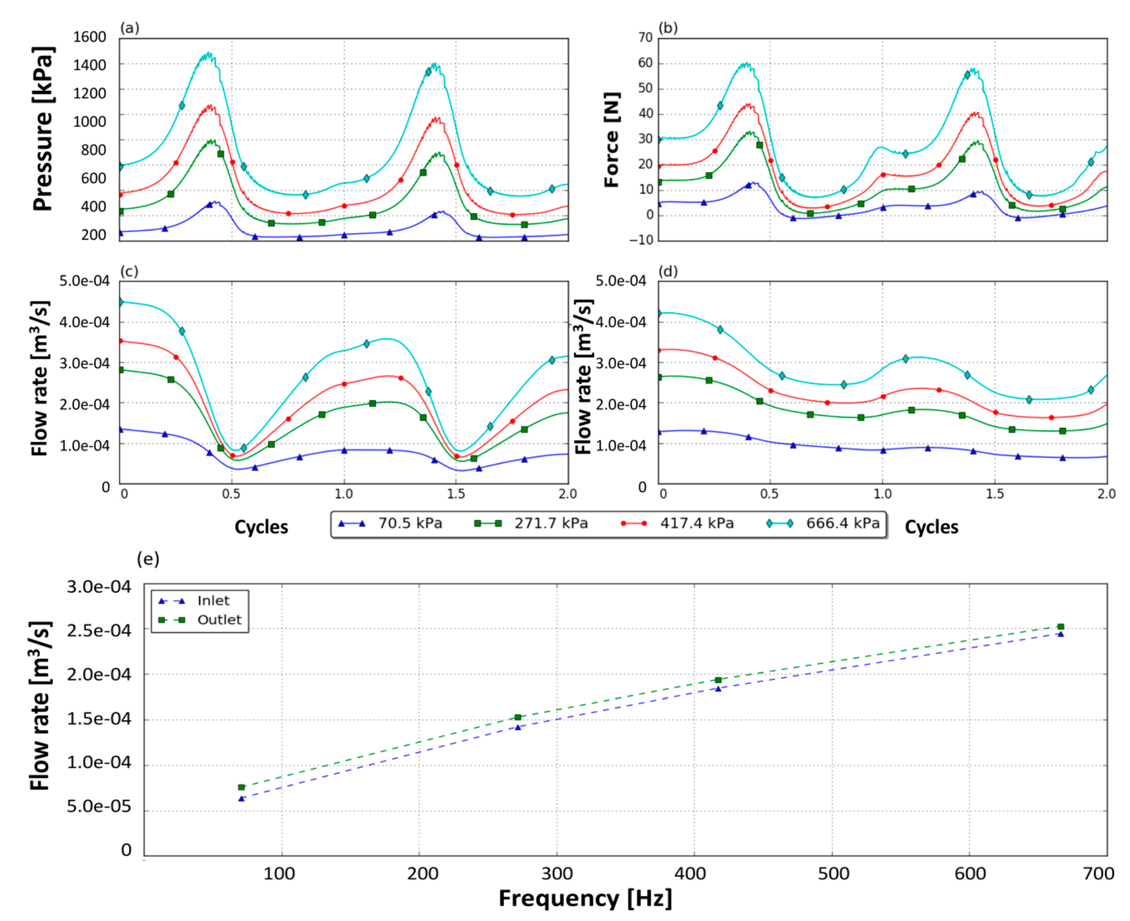
Figure 8 displays the pressure gradient for four portions of the cycle when the poppet is closing and opening using a sinusoidal input at 25 Hz. It was observed that during the closing process the pressure difference between port 1 and the connection to port 2 is greater than during the opening process. The pressure drop, flow forces on the poppet and flow rates at various frequencies are shown in Figure 9 for an inlet pressure of 666.4 kPa and several poppet frequencies. The pressure drop increased for higher cycle frequencies, as did the forces on the poppet, especially during the closing of the poppet. Peak forces on the poppet were double between poppet frequency of 25 Hz and 200 Hz. Flow rates decrease with higher poppet frequencies and with respect to the steady state simulations, which was expected.
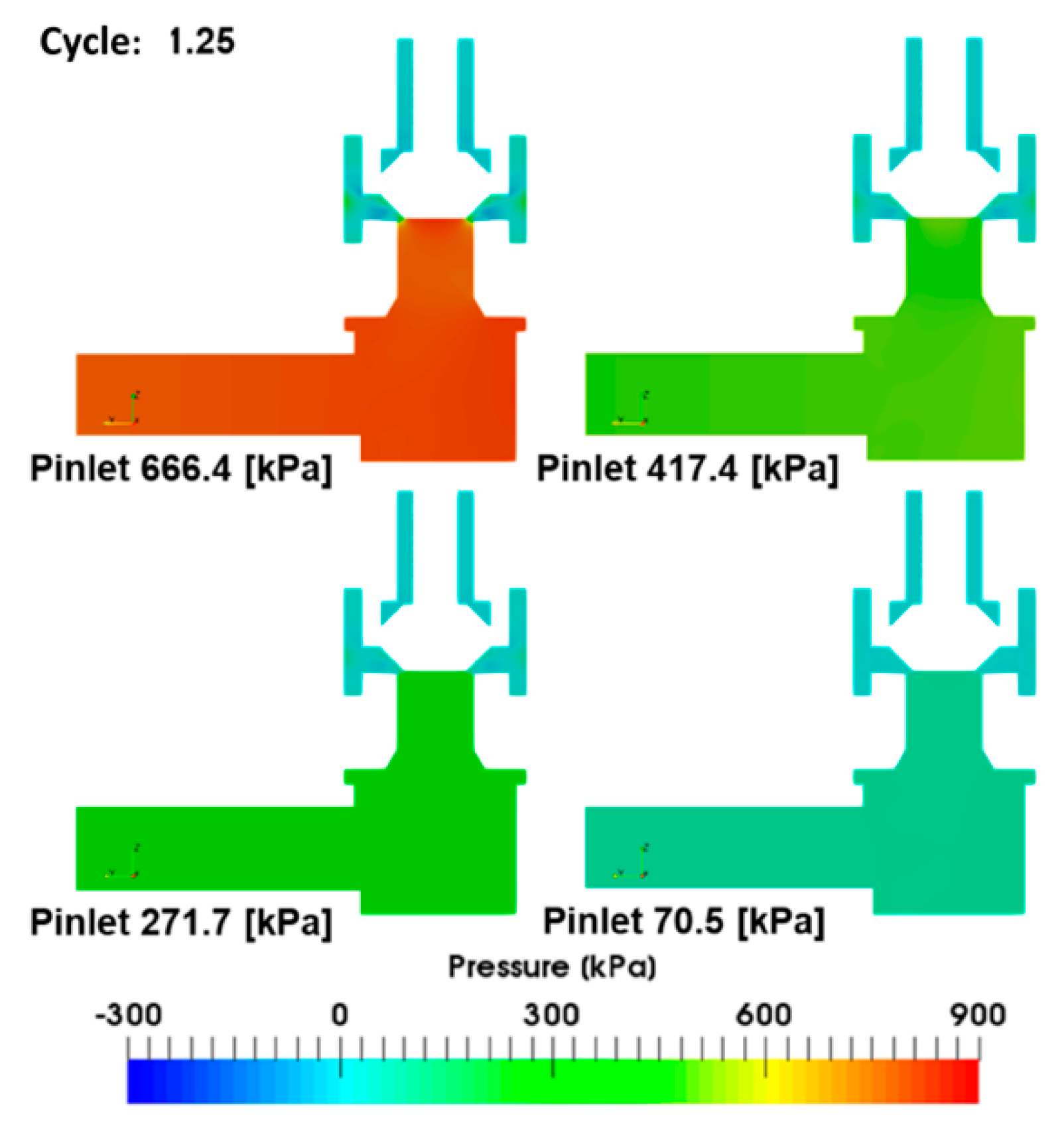
Figure 10 depicts the pressure gradient for frequencies between 25 Hz and 200 Hz at a timing of one a quarter cycle. It is worth noting that the pressure result at port 2 (outlet) seems to be unaffected by poppet frequency and increase pressure buildup is occurring mainly upstream.
Figure 11 depicts the differential pressure and net force on the poppet and flow rates at the inlet and outlet of ports 1 and 2 when the valve is operated at 200 Hz and a range of inlet pressures. Similar to the steady state behavior, it was observed that the pressure drop across the two ports increased with increasing inlet pressure. This behavior is consistent for all studied frequencies. The results can be used to estimate the required force necessary to close the poppet. It was observed that the force required to close the poppet increases sixfold between an inlet pressure of 70.5 kPa and 666.4 kPa. The flow rate decreases as the frequency is increased.
It can be observed in Figure 12 that pressure gradients decrease as inlet pressure decreases. The simulated pressure values for port 1 were between 70.5 kPa and 666.4 kPa. As inlet pressure increases velocity also increases and the pressures in port 2 are maintained between 5 kPa and 20 kPa. At an inlet pressure of 666.4 kPa, vortices were observed, which created low pressure points with values of −5 kPa to 15 kPa.
3.2.3. Non-dimensional Analysis
The previous Section highlights the overall complexities involved in the interaction between all parameters involved in the valve dynamics at high frequencies. A non-dimensional analysis of the system behavior was performed for the purpose of obtaining a general representation of the results. It is assumed that the pressure drop dp is a function of the valve geometry and the flow properties. Therefore the pressure drop can be expressed in terms of the relevant variables as:
where Q is the average flow rate, f is the poppet displacement frequency, μ is the viscosity of the fluid, ρ is the density of the fluid, and D is the diameter at the inlet for port 1. The non-dimensional analysis leads to three dimensionless numbers.
Figure 13 shows the results of the evaluation of the non-dimensional numbers at the flow conditions presented in the previous Section. The curves characterize the behavior of the non-dimensional pressure drop πdp as a function of the non-dimensional flow rate πQ for several frequencies related to the non-dimensional number πf.
Figure 13 shows that there is a direct relationship between πdp and πQ. Increasing the non-dimensional frequency number πf increases the slope in the πdp and πQ relationship. As the working frequency is increased the flow losses increase at a given flow rate. Numerically speaking, if the pressure drop is required to be kept constant at higher frequency of operation, it would be necessary to decrease the flow rate, for instance for a constant πdp = 8 × 10⁷ it would be required to decrease the flow rate by more than 50% to increase the frequency from 25 to 200 Hz. Using the non-dimensional numbers from Equation (13) and the plot in Figure 13, it could be inferred that implementing changes in some of the parameters of the valve or the operating conditions could lead to an improved valve dynamic behavior without incurring an increase in pressure loss. For example, decreasing the viscosity of the fluid is an effective way to be able to operate the valve at higher frequencies and flow rates due to the quadratic response between this constant and the πdp number. Increasing the diameter at port 1 would slightly decrease the flow and would increase moderately the pressure drop, at higher frequencies.
3.2.4. Evaluation of Variation of the Poppet Angle
The seat and poppet angle were another design parameter used to evaluate the sensitivity of the model. Angles lower than the commercial poppet were tested to study the effect on pressure drop and flow forces during closing and opening events. Figure 14 depicts various representations of the redesigned poppet geometries. The change in angle was implemented insuring the poppet displacement remained unchanged and guaranteeing that the clearance between the poppet and the seat was maintained to minimize pressure losses at valve closing.
The results for the variation of the poppet angle are depicted in Figure 15. It was found that the angle has minimal effect on pressure differential, the maximum values obtained were between 107 kPa to 110 kPa, which are less than a 1% change with respect to the original poppet angle.
Similarly, changes in the flow rate at the inlet and outlet where not significant. However, the flow forces during the entire motion of the poppet were seen to increase as the angles were decreased, which from an energetic perspective allows us to conclude that reducing the poppet angle is undesirable because it would lead to larger power requirements for actuation of the valve.
Figure 16 shows the pressure gradients for the closing process, it can be seen from the Figure that as the angle is reduced, negative pressure zones were reduced, which is associated with larger changes in the flow direction at port 2, leading to accelerated flows during the closing of port 1. This is assumed to be the principal cause for the increase in flow forces for lower angles. This is considered to be a local phenomenon, meaning it only affects the velocity, pressure and force around the poppet, but does not affect global variables such as inlet and outlet flow and pressure differential.
4. Conclusions
A model able to simulate the flow through a poppet valve was developed. The model was validated by comparing the pressure drop at different flow rates and comparing with data provided by the manufacturer of the valve. Values within 5% error were obtained for most flow rates. The model is also able to model the dynamic behavior of the valve as the poppet opens and closes cyclically at different frequencies.
The model was used to characterize the behavior of the flow through the valve as frequencies increased from 25 Hz to 200 Hz. It was established that as frequency of operation of the valve increased flow rate decreased. Also, forces on the poppet, related to the force needed to actuate the valve, increased with increasing frequencies. For example, at the higher inlet pressure studied, force increased twofold as frequency went from 25 Hz to 200 Hz.
In order to obtain more general results and to gain better insight on the process, a non-dimensionalized parametric study revealed that changes in the fluid’s viscosity or the diameter of the ports could effectively improve the performance of the valve. The analysis showed that as frequency increased, the slope of the relation between pressure drop and flow rate became steeper. This means that increasingly higher pressure drops occurred for a given flow rate as frequency increased. It was shown that pressure drop under particular conditions were proportional to the square of the viscosity and inversely proportional to the square of the diameter of the ports. Taking these parameters into consideration may allow to design poppet valves systems that are able to operate at higher frequencies. Finally, it was shown that poppet angle had little effect on the overall performance of the system.
In order to continue improving the understanding of the overall behavior of poppet valves at high frequencies and improve the design of such valves to make them capable of operating at high frequencies, it would be interesting to couple the current model with that of the solenoid responsible for operating the valve. This will allow to incorporate the response of that system into the overall time response of the valve.
The current model can also aid in analyzing novel designs that are able of reducing pressure drop and force on the poppet at high frequencies.
Author Contributions
Conceptualization, A.G.-M. and J.G.-B.; methodology, I.G., J.G.-B. and A.G.-M.; software, A.G.-M. and I.G.; validation, I.G., J.G.-B. and A.G.-M.; formal analysis, I.G.; investigation, I.G.; resources, I.G.; data curation, I.G.; writing—original draft preparation, I.G. and J.G.-B.; writing—review and editing, I.G., J.G.-B., B.N. and A.G.-M.; visualization, I.G.; supervision, A.G.-M. and J.G.-B.
Funding
This research received no external funding.
Conflicts of Interest
The authors declare no conflict of interest.
Nomenclature
| A | Total movement amplitude of the poppet |
| C | Empirical constant for the wall boundary |
| De | Valve delay |
| dp | Pressure drop across de valve |
| E | Empirical constant for wall boundary |
| f | Valve oscillation frequency |
| I | Turbulence intensity |
| K | von Karman constant |
| Kh | Velocity factor for the change of head-viside function |
| P(t) | Valve position function |
| Total pressure, average and fluctuating | |
| Q | Port 1 flow rate |
| t | Time |
| Total velocity, average and fluctuating | |
| U+ | Non-dimensional velocity |
| Y+ | Non-dimensional distance to the wall |
| κ | Turbulence energy |
| μ | Dynamic viscosity |
| μt | Turbulence viscosity |
| πdp | Loss number |
| πf | Frequency number |
| πQ | Flow number |
| ρ | Fluid’s density |
| Total Stress tensor, average, fluctuating |
References
- Eaton, Industrial Hydraulics Manual: Your Comprehensive Guide to Industrial Hydraulics; Eaton Hydraulics: Minneapolis, MN, USA, 2008; p. 642.
- Byington, C.; Watson, M. A model-based approach to prognostics and health management for flight control actuators. Aerosp. Conf. Proc. 2004, 6, 3551–3562. [Google Scholar]
- Smith, M.; Byington, C.; Watson, M.; Bharadwaj, S.; Swerdon, G.; Goebel, K.; Balaban, E. Experimental and analytical development of health management for Electro-Mechanical Actuators. In Proceedings of the IEEE Aerospace conference, Big Sky, MT, USA, 7–14 March 2009. [Google Scholar]
- De Oliveira Bizarria, C.; Yoneyama, T. Prognostics and Health Monitoring for an electro-hydraulic flight control actuator. In Proceedings of the IEEE Aerospace Conference, Big Sky, MT, USA, 7–14 March 2009. [Google Scholar]
- Mintsa, H.; Member, J.; Venugopal, R. Adaptive Control of an Electrohydraulic Position Servo System. In Proceedings of the IEEE AFRICON, Nairobi, Kenya, 23–25 September 2009. [Google Scholar]
- Paloniitty, M.; Linjama, M. High-Linear Digital Hydraulic Valve Control by an Equal Coded Valve System and Novel Switching Schemes. Proc. Inst. Mech. Eng. Part I J. Syst. Control Eng. 2018, 3, 258–269. [Google Scholar] [CrossRef]
- Porciúncula, G.; De Negri, V.; Dias, A. Reliability of Electro-Hydraulic Equipment: Systematization and Analysis. Proc. COBEM Int. Congress Mech. Eng. 2005, 2, 393–400. [Google Scholar]
- Villalobos, O.; Burvill, C.; Stecki, J. Fault Diagnosis of Electrohydraulic Systems. Proc. Jfps Int. Symp. Fluid Power 2005, 6, 658–663. [Google Scholar] [CrossRef]
- Long, G. Comparison Study of Position Control with 2-Way and 3-Way High Speed on/off Electrohydraulic Valves. Master’s Thesis, Purdue University, West Lafayette, IN, USA, 2009. [Google Scholar]
- Williamson, C.; Ivantysynova, M. Pump Mode Prediction For Four-Quadrant Velocity Control Of Valveless Hydraulic Actuators. In Proceedings of the 7th JFPS International Symposium on Fluid Power, Toyama, Japan, 11–15 September 2008. [Google Scholar]
- Ivantysynova, M. Innovations in Pump Design-What Are Future Directions? In Proceedings of the JFPS International Symposium on Fluid Power, Toyama, Japan, 11–15 September 2008; pp. 59–64. [Google Scholar]
- Eggers, B.; Rahmfeld, R.; Ivantysynova, M. An Energetic Comparison Between Valveless and Valve Controlled Active Vibration Damping for Off-Road Vehicles. Proc. Jfps Int. Symp. Fluid Power 2005, 6, 275–283. [Google Scholar] [CrossRef]
- Andruch, J.; Lumkes, J. A hydraulic system topography with integrated energy recovery and reconfigurable flow paths using high speed valves. In Proceedings of the 51st National Conference on Fluid Power (NCFP), Las Vegas, NV, USA, 12–14 March 2008; pp. 649–657. [Google Scholar]
- Opdenbosch, P.; Sadegh, N.; Book, W.; Enes, A. Auto-calibration based control for independent metering of hydraulic actuators. In Proceedings of the IEEE International Conference on Robotics and Automation, Shanghai, China, 9–13 May 2011; pp. 153–158. [Google Scholar]
- Guglielmino, E.; Semini, C.; Kogler, H.; Scheidl, R.; Caldwell, D. Power Hydraulics—Switched Mode Control of Hydraulic Actuation. In Proceedings of the IEEE/RSJ International Conference on Intelligent Robots and Systems, Taipei, Taiwan, 18–22 October 2010; pp. 3031–3036. [Google Scholar]
- Linjama, M.; Vilenius, M. Digital hydraulics—Towards perfect valve technology. In Proceedings of the Tenth Scandinavian International Conference on Fluid Power, Tampere, Finland, 21–23 May 2007; pp. 2–16. [Google Scholar]
- Tu, H.; Rannow, M.; Van De Ven, J.; Wang, M.; Li, P.; Chase, T. High Speed Rotary Pulse Width Modulated On/Off Valve. In ASME 2007 International Mechanical Engineering Congress and Exposition; American Society of Mechanical Engineers: Seattle, WA, USA, 11–15 November 2007; pp. 1–14. [Google Scholar]
- Schepers, I.; Schmitz, D.; Weiler, D.; Cochoy, O.; Neumann, U. A novel model for optimizing development and application of switching valves in closed loop control. Int. J. Fluid Power 2011, 12, 31–40. [Google Scholar] [CrossRef]
- Wang, Q.; Yang, F.; Yang, Q.; Chen, J.; Guan, H. Experimental analysis of new high-speed pow-erful digital solenoid valves. Energy Convers. Manag. 2011, 52, 2309–2313. [Google Scholar]
- Pindera, M.; Sun, Y.; Malosse, J.; Garcia, J. Co-Simulation Based Design and Experimental Validation of Control Strategies for Digital Fluid Power Systems. In Proceedings of the ASME/BATH Symposium on Fluid Power and Motion Control, Sarasota, FL, USA, 6–9 October 2013; p. V001T01A053. [Google Scholar]
- Paloniitty, M.; Linjama, M.; Huhtala, K. Equal coded digital hydraulic valve system—Improving tracking control with pulse frequency modulation. Procedia Eng. 2015, 106, 83–91. [Google Scholar] [CrossRef]
- Van Varseveld, R.; Bone, G. Accurate position control of a pneumatic actuator using on/off solenoid valves. IEEE/ASME Trans. Mechatron. 1997, 2, 195–204. [Google Scholar] [CrossRef]
- Xu, B.; Ding, R.; Zhang, J.; Su, Q. Modeling and dynamic characteristics analysis on a three- stage fast-response and large-flow directional valve. Energy Convers. Manag. 2014, 79, 187–199. [Google Scholar] [CrossRef]
- Jackson, R.; Belger, M.; Cassaidy, K.; Kokemoor, A. CFD simulation and experimental investigation of steady state flow force reduction in a hydraulic spool valve with machined back angles. In Proceedings of the ASME/BATH Symposium on Fluid Power and Motion Control, Sarasota, FL, USA, 16–19 October 2017. [Google Scholar]
- Tian, H.; Van de Ven, J. Geometric optimization of a hydraulic motor rotary valve. In Proceedings of the ASME/BATH Symposium on Fluid Power and Motion Control, Sarasota, FL, USA, 6–9 October 2013. [Google Scholar]
- Finesso, R.; Rundo, M. Numerical and experimental investigation on a conical poppet relief valve with flow force compensation. Int. J. Fluid Power 2017, 18, 111–122. [Google Scholar] [CrossRef]
- Han, M.; Liu, Y.; Wu, D.; Zhao, X.; Tan, H. A numerical investigation in characteristics of flow force under cavitation state inside the water hydraulic poppet valves. Int. J. Heat Mass Transfer 2017, 111, 1–16. [Google Scholar] [CrossRef]
- Duan, Y.; Jackson, C.; Eaton, M.; Bluck, M. An assessment of eddy viscosity models on predicting performance parameters of valves. Nucl. Eng. Des. 2019, 342, 60–77. [Google Scholar] [CrossRef]
- Lisowski, E.; Rajda, J. CFD analysis of pressure loss during flow by hydraulic directional control valve constructed from logic valves. Energy Convers. Manag. 2013, 65, 285–291. [Google Scholar] [CrossRef]
- Lisowski, E.; Czyzycki, W.; Rajda, J. Three dimensional CFD analysis and experimental test of flow force acting on the spool of solenoid operated directional control valve. Energy Convers. Manag. 2013, 70, 220–229. [Google Scholar] [CrossRef]
- ISO 4411:2008(E), Hydraulic Fluid Power—Valves—Determination of Pressure Differential/Flow Characteristics Standard; International Organization for Standardization: Geneva, Switzerland, 2008.
- Sun Hydraulics. Performance Data, Accumulator Sense, Pump Unload Valves | Sun Hydraulics. 2019. Available online: www.sunhydraulics.com/tech-resources/performance-data (accessed on 23 February 2019).
- Duan, Y.; Revell, A.; Sinha, J.; Hahn, W. A study of unsteady force on the stem in a valve with different openings. In Proceedings of the 1st International Conference Maintenance Engineering, Manchester, UK, 30 August 2016; pp. 1–11. [Google Scholar]
- Duan, Y.; Revell, A.; Sinha, J.; Hahn, W. Flow induced excitations in the high pressure steam turbine governor valve at different openings. In Proceedings of the 2nd International Conference Maintenance Engineering, Manchester, UK, 5–6 September 2017; pp. 1–13. [Google Scholar]
Figure 1.
Representation of the implemented valve: (a) ISO schematic representation; (b) picture of the valve cartridge; (c) detailed Section using a CAD model.
Figure 1.
Representation of the implemented valve: (a) ISO schematic representation; (b) picture of the valve cartridge; (c) detailed Section using a CAD model.

Figure 2.
Scaled down representation of the physical model domain at 45°.

Figure 3.
Diagram of implemented boundary conditions.

Figure 4.
Detail of elements generated using the “layering” tool in ANSYS.

Figure 5.
Comparison between pressure differential from the simulation and the manufacturer’s data.

Figure 6.
Transient analysis of poppet displacement.

Figure 7.
Dynamic analysis of pressure differential for opening, closing procedures and fluctuating positions.
Figure 7.
Dynamic analysis of pressure differential for opening, closing procedures and fluctuating positions.

Figure 8.
Pressure gradients at various cycle timings for 25 Hz during closing and opening procedures.
Figure 8.
Pressure gradients at various cycle timings for 25 Hz during closing and opening procedures.

Figure 9.
Simulated results at various frequencies for 666.4 kPa inlet pressure, (a) pressure differential, (b) net force on the poppet, (c) inlet flow, (d) outlet flow, (e) average inlet and outlet flows for second cycle.
Figure 9.
Simulated results at various frequencies for 666.4 kPa inlet pressure, (a) pressure differential, (b) net force on the poppet, (c) inlet flow, (d) outlet flow, (e) average inlet and outlet flows for second cycle.

Figure 10.
Pressure gradients during second cycle at 1.25 timing for various frequencies during the closing procedure.
Figure 10.
Pressure gradients during second cycle at 1.25 timing for various frequencies during the closing procedure.

Figure 11.
Simulated results at 200 Hz for varying inlet pressures, (a) pressure differential, (b) net force on the poppet, (c) inlet flow, (d) outlet flow, (e) average inlet and outlet flows for second cycle.
Figure 11.
Simulated results at 200 Hz for varying inlet pressures, (a) pressure differential, (b) net force on the poppet, (c) inlet flow, (d) outlet flow, (e) average inlet and outlet flows for second cycle.

Figure 12.
Pressure gradients during second cycle for the closing procedure at varying flow rates (flow velocity).
Figure 12.
Pressure gradients during second cycle for the closing procedure at varying flow rates (flow velocity).

Figure 13.
Non-dimensionalized valve parameter relations.

Figure 14.
Poppet valve angles evaluated in the simulation.

Figure 15.
Simulated results for a 25 Hz operating frequency and a 666.4 kPa inlet pressure. (a) Pressure differential, (b) net force on the poppet, (c) inlet flow, (d) outlet flow.
Figure 15.
Simulated results for a 25 Hz operating frequency and a 666.4 kPa inlet pressure. (a) Pressure differential, (b) net force on the poppet, (c) inlet flow, (d) outlet flow.

Figure 16.
Simulated pressure gradient for closing event using various poppet angles.


Table 1.
Properties of the fluid used in the simulation.
| Material | Temperature (°C) | Density (kg/m3) | Dynamic Viscosity (kg·m/s) |
|---|---|---|---|
| Oil AW 32 | 49 | 847.8 | 0.0195 |
Table 2.
Summary of results for mesh convergence tests.
| Elements | Published Pressure (kPa) | Simulated Pressure (kPa) | Percent Error |
|---|---|---|---|
| 3,970,308 | 540 | 603 | 11.70% |
| 5,512,452 | 540 | 588 | 8.98% |
| 8,239,820 | 540 | 576 | 6.72% |
| 9,864,461 | 540 | 576 | 6.96% |
| 12,308,409 | 540 | 574 | 6.45% |
Table 3.
Summary of results for turbulence and wall function tests.
| Turbulence Model | Published Pressure (kPa) | Simulated Pressure (kPa) | Percent Error |
|---|---|---|---|
| Standard κ-ε | 540 | 577 | 6.96% |
| Standard κ-ε SWF | 540 | 531 | 1.50% |
| Standard κ-ε EWT | 540 | 543 | 0.61% |
| Realizable κ-ε SWT | 540 | 484 | 10.34% |
| Realizable κ-ε EWT | 540 | 550 | 1.94% |
| κ-ω SST | 540 | 607 | 12.6% |
| Spalart-Allmaras | 540 | 577 | 3.45% |
Table 4.
Summary of pressure differential from static simulation at various flow velocities.
| Flow Rate (m3/s) | Published Pressure (kPa) | Simulated Pressure (kPa) | Percent Error |
|---|---|---|---|
| 4.44 × 10⁻⁴ | 540 | 559 | 3.59% |
| 3.76 × 10⁻⁴ | 389 | 404 | 3.96% |
| 3.01 × 10⁻⁴ | 252 | 262 | 4.08% |
| 2.24 × 10⁻⁴ | 144 | 148 | 3.07% |
| 1.47 × 10⁻⁴ | 64 | 67 | 5.42% |
| 6.75 × 10⁻⁵ | 14 | 16 | 14.83% |
Table 5.
Parameters and levels analyzed for the transient state simulations.
| Parameter | 1 | 2 | 3 | 4 |
|---|---|---|---|---|
| Frequency (Hz) | 25 | 50 | 100 | 200 |
| Inlet Pressure (kPa) | 70.5 | 271.7 | 417.3 | 666.4 |
© 2019 by the authors. Licensee MDPI, Basel, Switzerland. This article is an open access article distributed under the terms and conditions of the Creative Commons Attribution (CC BY) license (http://creativecommons.org/licenses/by/4.0/).
Share and Cite
MDPI and ACS Style
Gomez, I.; Gonzalez-Mancera, A.; Newell, B.; Garcia-Bravo, J. Analysis of the Design of a Poppet Valve by Transitory Simulation. Energies 2019, 12, 889. https://doi.org/10.3390/en12050889
AMA Style
Gomez I, Gonzalez-Mancera A, Newell B, Garcia-Bravo J. Analysis of the Design of a Poppet Valve by Transitory Simulation. Energies. 2019; 12(5):889. https://doi.org/10.3390/en12050889
Chicago/Turabian StyleGomez, Ivan, Andrés Gonzalez-Mancera, Brittany Newell, and Jose Garcia-Bravo. 2019. "Analysis of the Design of a Poppet Valve by Transitory Simulation" Energies 12, no. 5: 889. https://doi.org/10.3390/en12050889
Note that from the first issue of 2016, this journal uses article numbers instead of page numbers. See further details here.